04/10/25 Image Compression3 Objective • Reduce the number of bytes required to represent a digital image – Redundant data reduction – Remove patterns – Uncorrelated data confirms redundant data elimination • Auto correlation?
4.
04/10/25 Image Compression4 Enabling Technology • Compressions is used in – FAX – RPV – Teleconference – REMOTE DEMO – etc
5.
04/10/25 Image Compression5 Review • What and how to exploit data redundancy • Model based approach to compression • Information theory principles • Types of compression – Lossless, lossy
6.
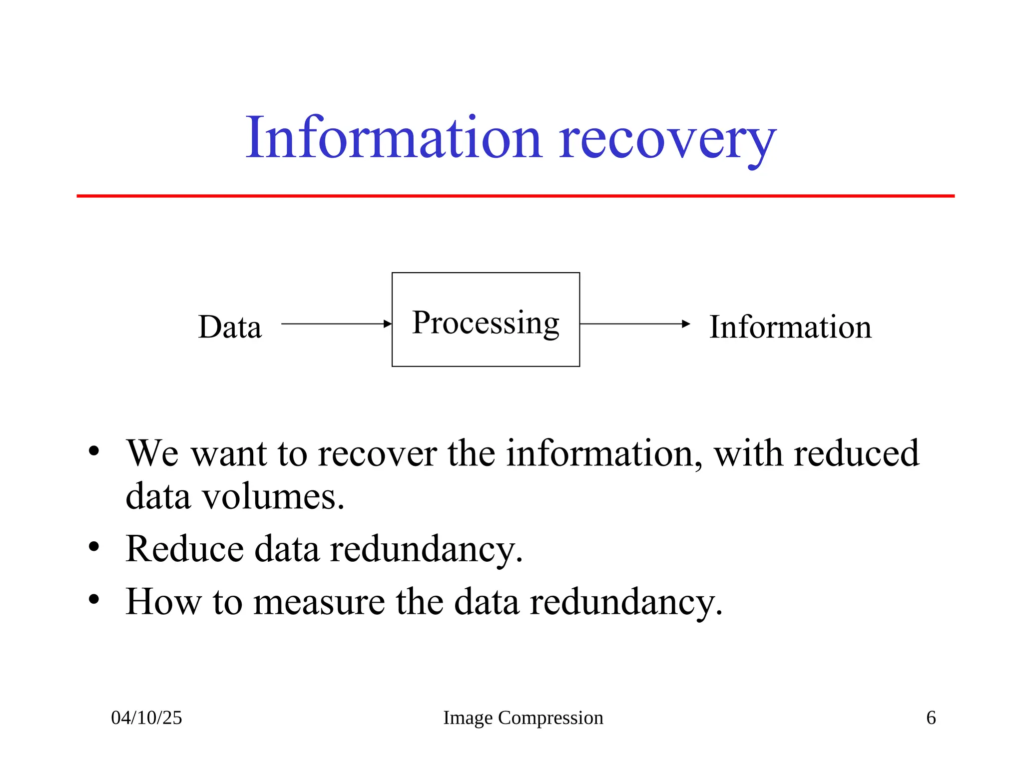
04/10/25 Image Compression6 Information recovery • We want to recover the information, with reduced data volumes. • Reduce data redundancy. • How to measure the data redundancy. Processing Data Information
7.
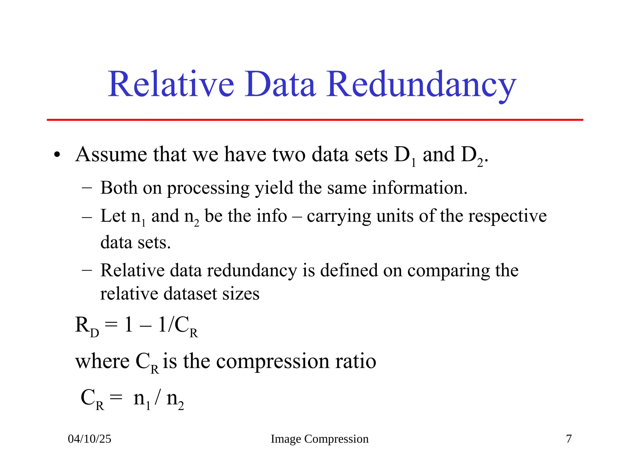
04/10/25 Image Compression7 Relative Data Redundancy • Assume that we have two data sets D1 and D2. – Both on processing yield the same information. – Let n1 and n2 be the info – carrying units of the respective data sets. – Relative data redundancy is defined on comparing the relative dataset sizes RD = 1 – 1/CR where CR is the compression ratio CR = n1 / n2
8.
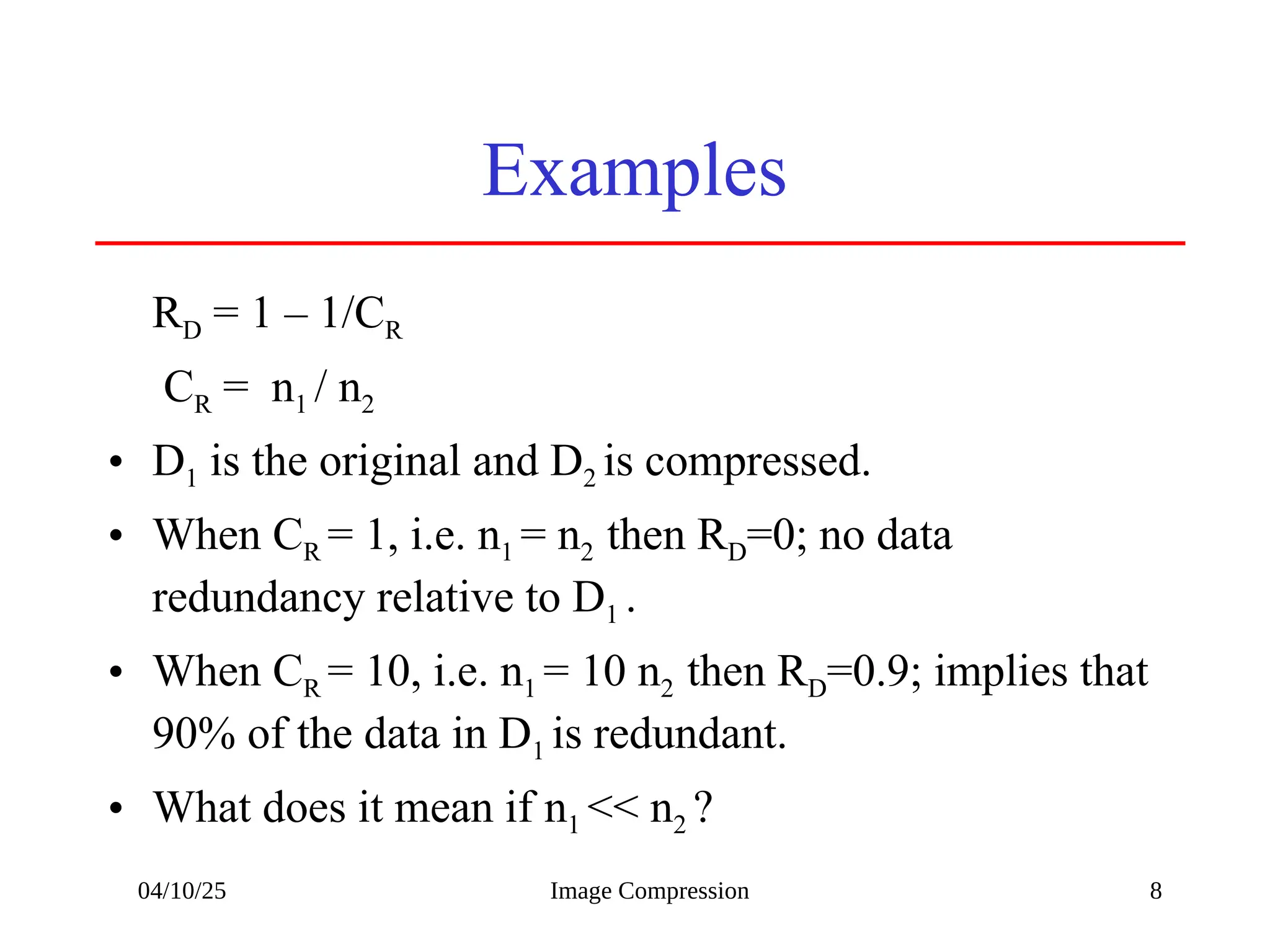
04/10/25 Image Compression8 Examples RD = 1 – 1/CR CR = n1 / n2 • D1 is the original and D2 is compressed. • When CR = 1, i.e. n1 = n2 then RD=0; no data redundancy relative to D1 . • When CR = 10, i.e. n1 = 10 n2 then RD=0.9; implies that 90% of the data in D1 is redundant. • What does it mean if n1 << n2 ?
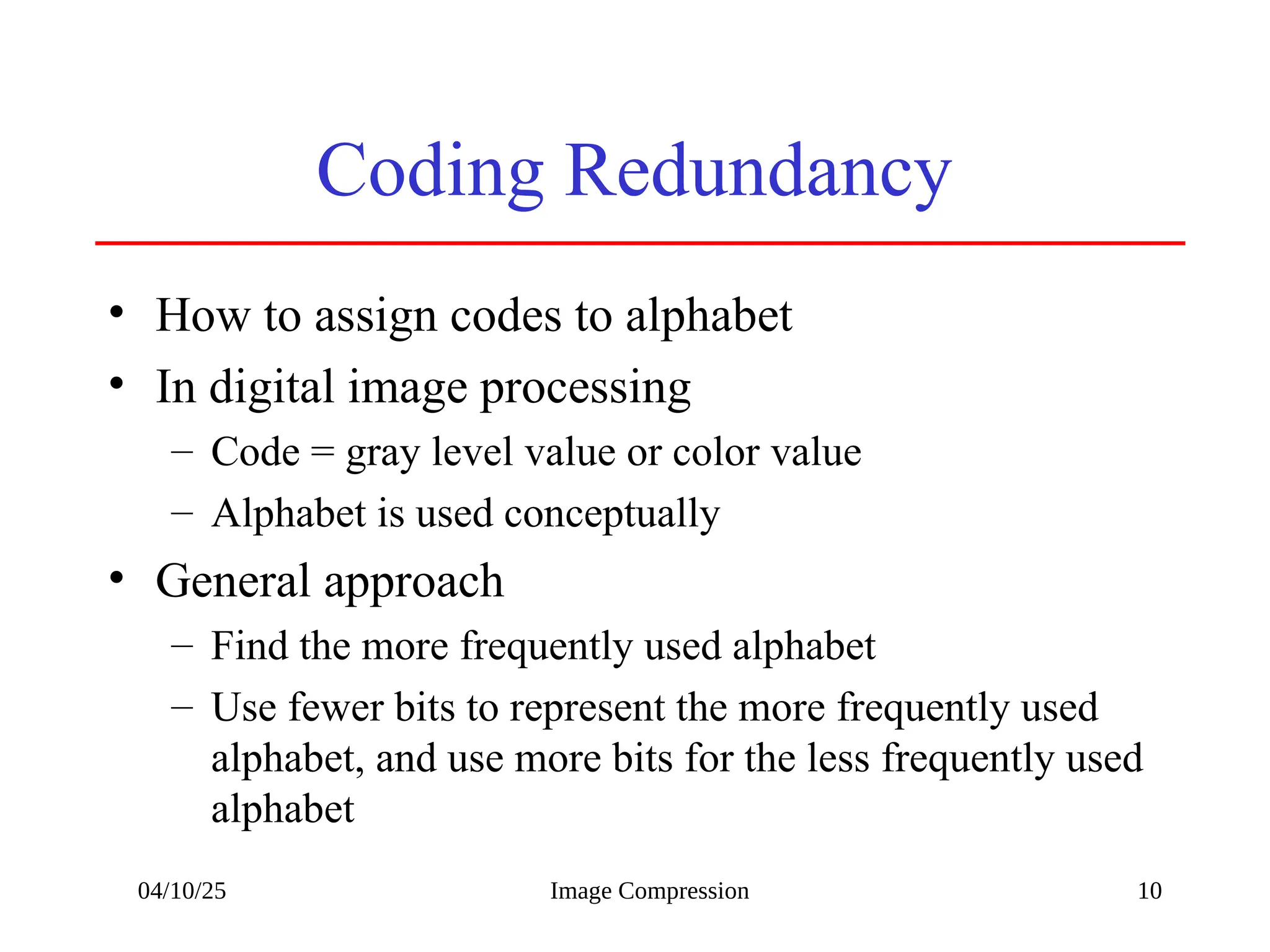
04/10/25 Image Compression10 Coding Redundancy • How to assign codes to alphabet • In digital image processing – Code = gray level value or color value – Alphabet is used conceptually • General approach – Find the more frequently used alphabet – Use fewer bits to represent the more frequently used alphabet, and use more bits for the less frequently used alphabet
11.
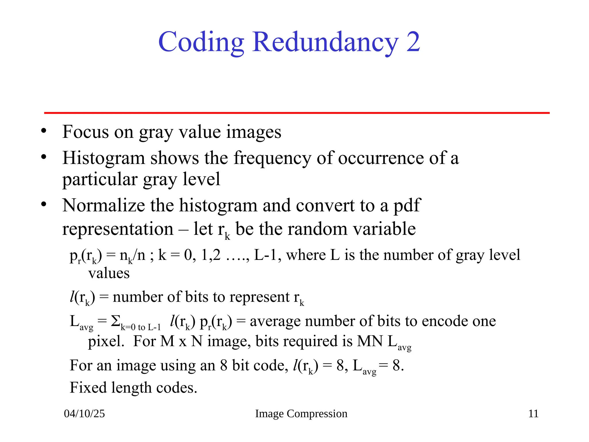
04/10/25 Image Compression11 Coding Redundancy 2 • Focus on gray value images • Histogram shows the frequency of occurrence of a particular gray level • Normalize the histogram and convert to a pdf representation – let rk be the random variable pr(rk) = nk/n ; k = 0, 1,2 …., L-1, where L is the number of gray level values l(rk) = number of bits to represent rk Lavg = k=0 to L-1 l(rk) pr(rk) = average number of bits to encode one pixel. For M x N image, bits required is MN Lavg For an image using an 8 bit code, l(rk) = 8, Lavg = 8. Fixed length codes.
04/10/25 Image Compression15 Run Length Coding From [1] CR=1024*343/12166*11 = 2.63 RD = 1-1/2.63 = 0.62
16.
04/10/25 Image Compression16 Psychovisual Redundancy • Some visual characteristics are less important than others. • In general observers seeks out certain characteristics – edges, textures, etc – and the mentally combine them to recognize the scene.
![04/10/25 Image Compression 2 Reference [1] Gonzalez and Woods, Digital Image Processing.](https://image.slidesharecdn.com/13-imagecompression-250410134217-1a054bb7/75/Image-CompressionImage-CompressionImage-CompressionImage-CompressionImage-CompressionImage-CompressionImage-CompressionImage-Compression-ppt-2-2048.jpg)
![04/10/25 Image Compression 12 Fixed vs Variable Length Codes From [1] Lavg = 2.7 CR= 3/2.7 = 1.11 RD = 1 – 1/1.11 = 0.099](https://image.slidesharecdn.com/13-imagecompression-250410134217-1a054bb7/75/Image-CompressionImage-CompressionImage-CompressionImage-CompressionImage-CompressionImage-CompressionImage-CompressionImage-Compression-ppt-12-2048.jpg)
![04/10/25 Image Compression 13 Code assignment view From [1]](https://image.slidesharecdn.com/13-imagecompression-250410134217-1a054bb7/75/Image-CompressionImage-CompressionImage-CompressionImage-CompressionImage-CompressionImage-CompressionImage-CompressionImage-Compression-ppt-13-2048.jpg)
![04/10/25 Image Compression 14 Interpixel Redundancy From [1]](https://image.slidesharecdn.com/13-imagecompression-250410134217-1a054bb7/75/Image-CompressionImage-CompressionImage-CompressionImage-CompressionImage-CompressionImage-CompressionImage-CompressionImage-Compression-ppt-14-2048.jpg)
![04/10/25 Image Compression 15 Run Length Coding From [1] CR=1024*343/12166*11 = 2.63 RD = 1-1/2.63 = 0.62](https://image.slidesharecdn.com/13-imagecompression-250410134217-1a054bb7/75/Image-CompressionImage-CompressionImage-CompressionImage-CompressionImage-CompressionImage-CompressionImage-CompressionImage-Compression-ppt-15-2048.jpg)
![04/10/25 Image Compression 17 From [1]](https://image.slidesharecdn.com/13-imagecompression-250410134217-1a054bb7/75/Image-CompressionImage-CompressionImage-CompressionImage-CompressionImage-CompressionImage-CompressionImage-CompressionImage-Compression-ppt-17-2048.jpg)
![04/10/25 Image Compression 18 From [1]](https://image.slidesharecdn.com/13-imagecompression-250410134217-1a054bb7/75/Image-CompressionImage-CompressionImage-CompressionImage-CompressionImage-CompressionImage-CompressionImage-CompressionImage-Compression-ppt-18-2048.jpg)
![04/10/25 Image Compression 20 Subjective scale From [1]](https://image.slidesharecdn.com/13-imagecompression-250410134217-1a054bb7/75/Image-CompressionImage-CompressionImage-CompressionImage-CompressionImage-CompressionImage-CompressionImage-CompressionImage-Compression-ppt-20-2048.jpg)
![04/10/25 Image Compression 21 Image Compression Model Run length JPEG Huffman From [1]](https://image.slidesharecdn.com/13-imagecompression-250410134217-1a054bb7/75/Image-CompressionImage-CompressionImage-CompressionImage-CompressionImage-CompressionImage-CompressionImage-CompressionImage-Compression-ppt-21-2048.jpg)