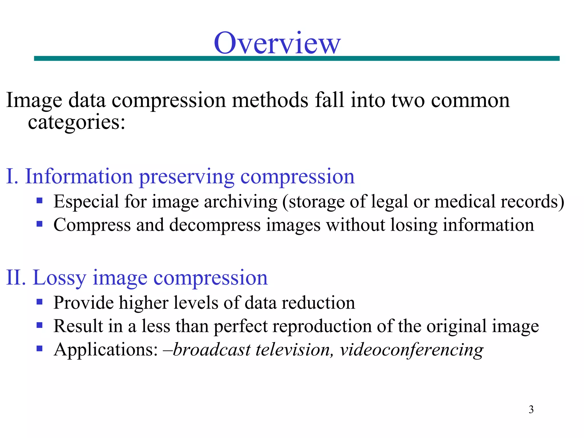
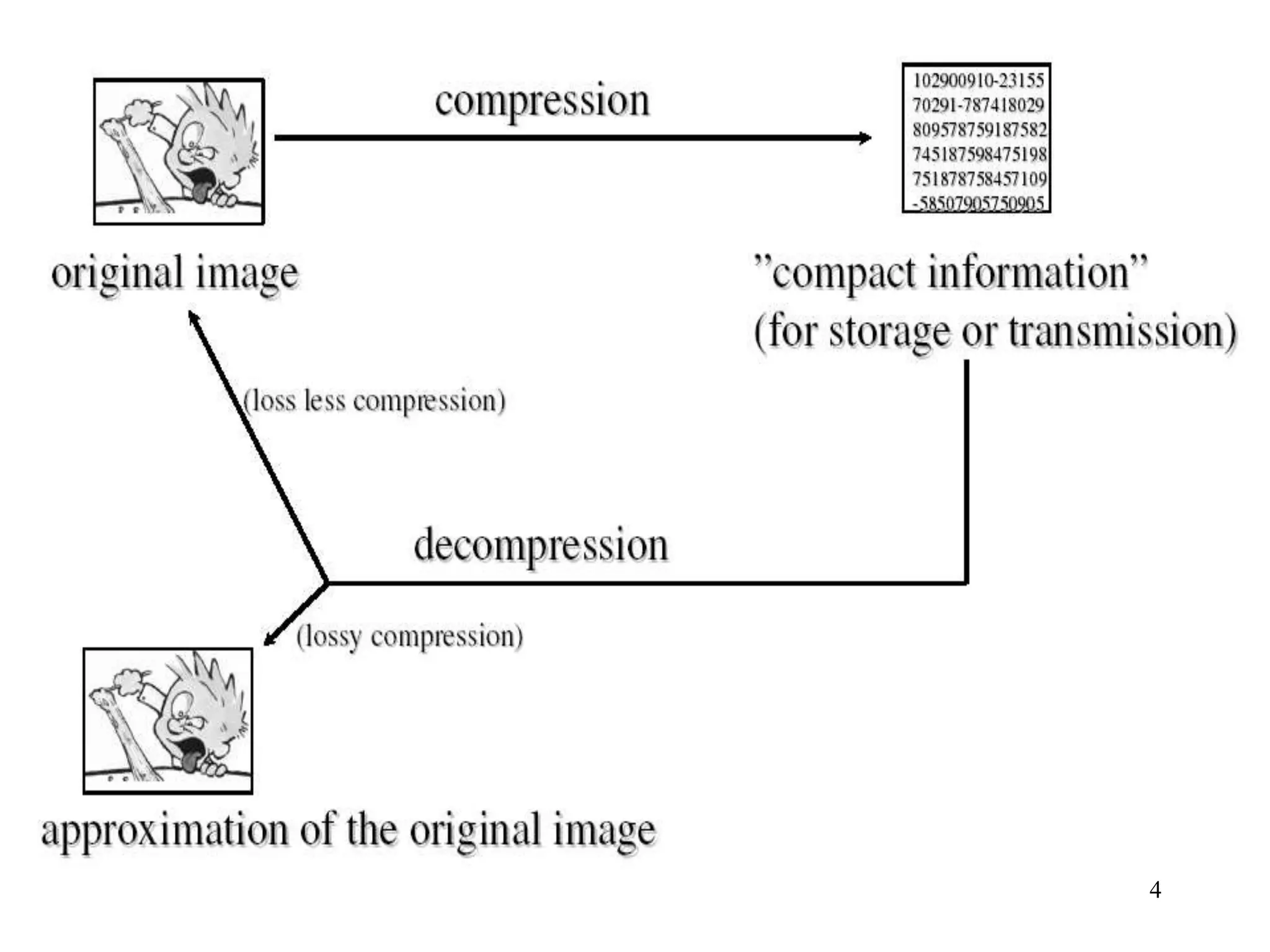
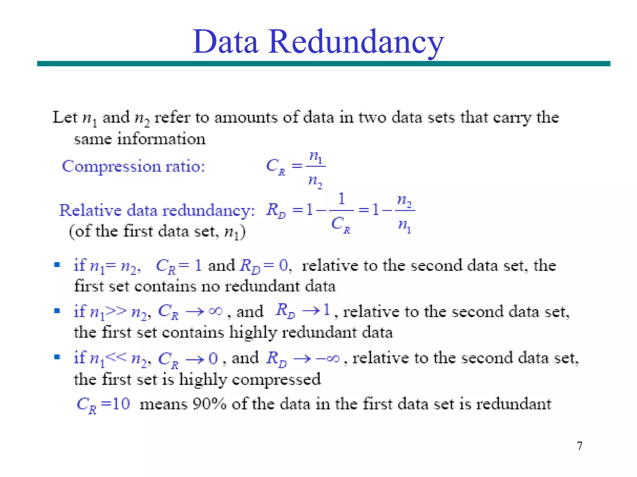
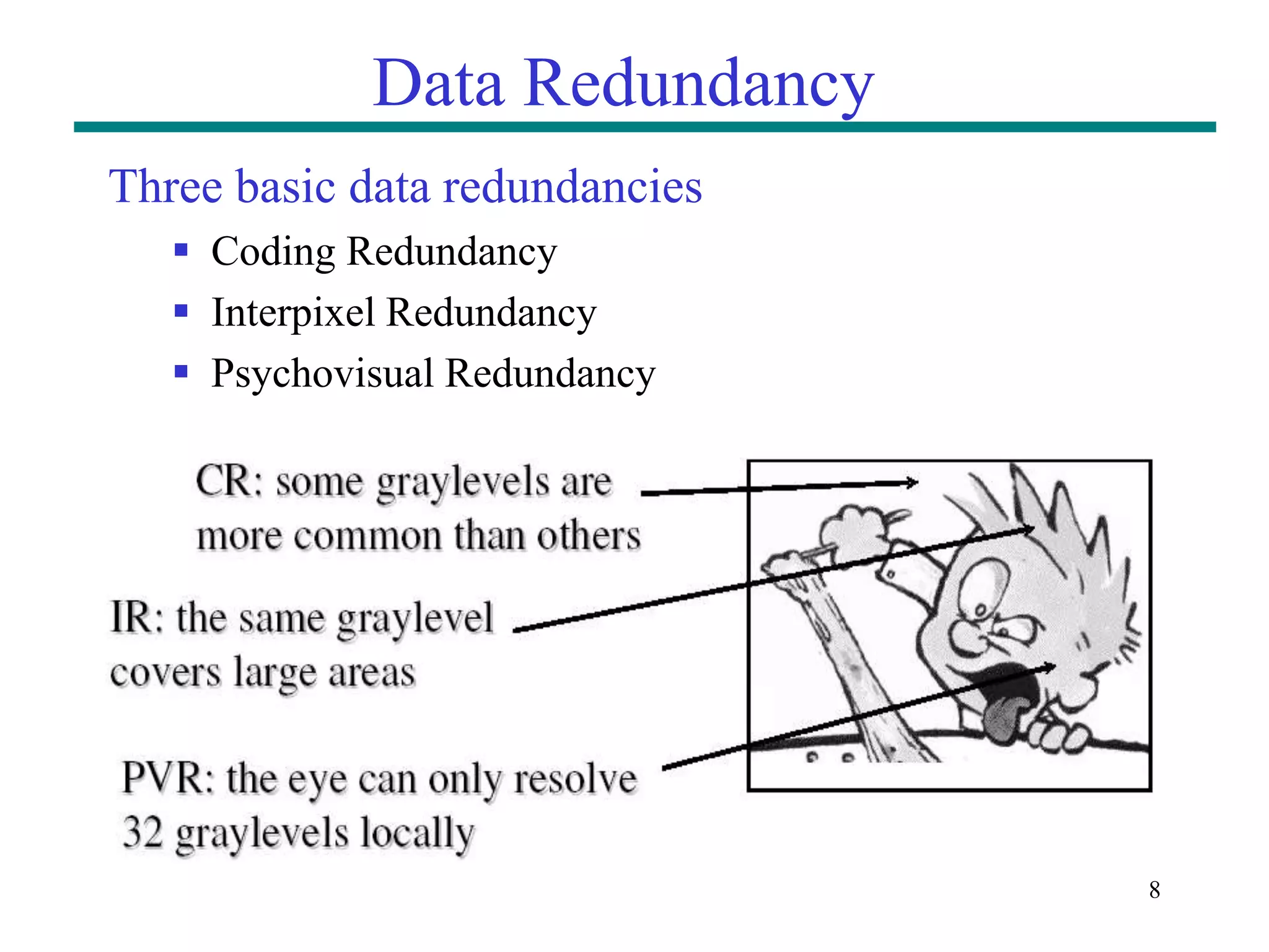
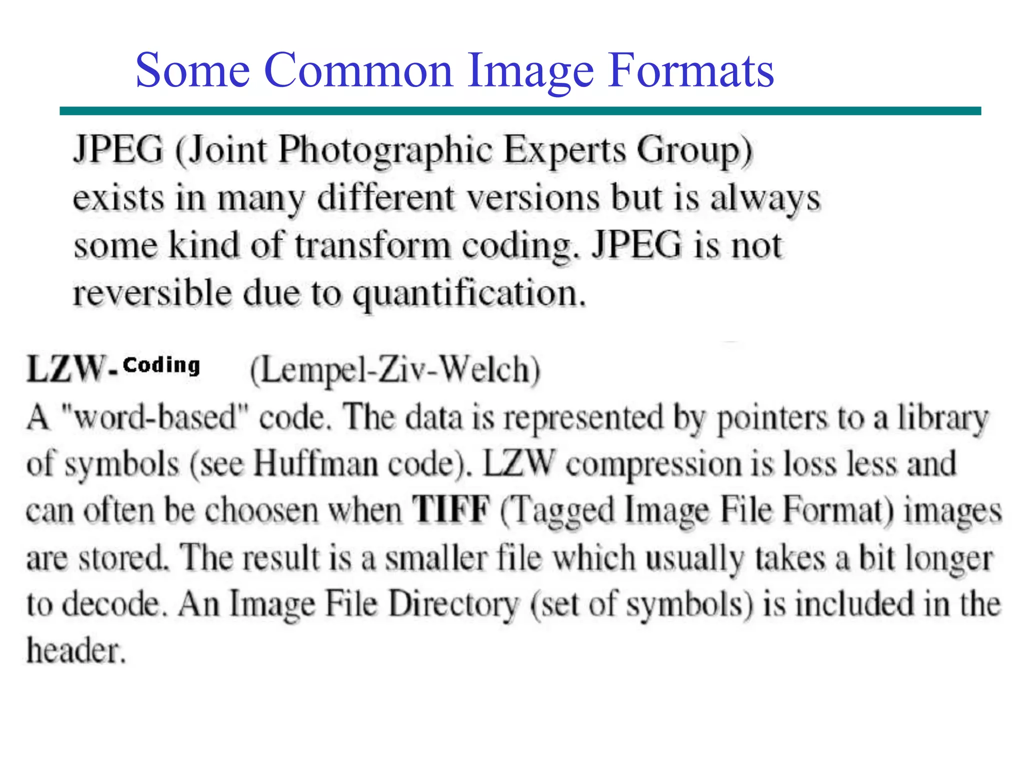
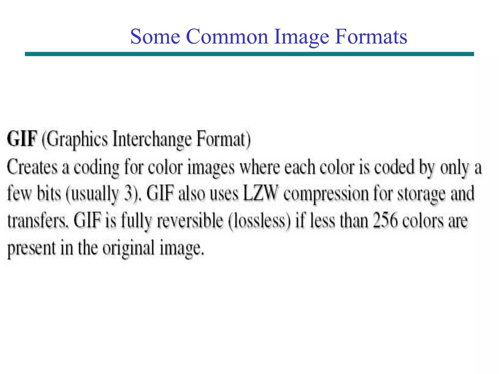
Digital Image Processing Image Compression Dr. Haris Masood
2 Background Principal objective: To minimize the number of bits required to represent an image. Applications Transmission: Broadcast TV via satellite, military communications via aircraft, teleconferencing, computer communications etc. Storage: Educational and business documents, medical images (CT, MRI and digital radiology), motion pictures, satellite images, weather maps, geological surveys, ...
3 Overview Image data compression methods fall into two common categories: I. Information preserving compression  Especial for image archiving (storage of legal or medical records)  Compress and decompress images without losing information II. Lossy image compression  Provide higher levels of data reduction  Result in a less than perfect reproduction of the original image  Applications: –broadcast television, videoconferencing
4
5 Data vs. information • Data is not the same thing as information • Data are the means to convey information; various amounts of data may be used to represent the same amount of information Part of data may provide no relevant information: data redundancy • The amount of data can be much larger expressed than the amount of information.
6 Data Redundancy • Data that provide no relevant information=redundant data or redundancy. • Image compression techniques can be designed by reducing or eliminating the Data Redundancy • Image coding or compression has a goal to reduce the amount of data by reducing the amount of redundancy.
7 Data Redundancy
8 Data Redundancy Three basic data redundancies  Coding Redundancy  Interpixel Redundancy  Psychovisual Redundancy
9 Coding Redundancy A natural m-bit coding method assigns m-bit to each gray level without considering the probability that gray level occurs with: Very likely to contain coding redundancy Basic concept:  Utilize the probability of occurrence of each gray level (histogram) to determine length of code representing that particular gray level: variable-length coding.  Assign shorter code words to the gray levels that occur most frequently or vice versa.
10 Coding Redundancy
11 Coding Redundancy (Example)
12 Coding Redundancy (Example)
13 Coding Redundancy (Example)
14 Interpixel Redundancy  Caused by High Interpixel Correlations within an image, i.e., gray level of any given pixel can be reasonably predicted from the value of its neighbors (information carried by individual pixels is relatively small) spatial redundancy, geometric redundancy, interframe redundancy (in general, interpixel redundancy )  To reduce the interpixel redundancy, mapping is used. The mapping scheme can be selected according to the properties of redundancy.  An example of mapping can be to map pixels of an image: f(x,y) to a sequence of pairs: (g1,r1), (g2,r2), ..., (gi,ri), .. gi: ith gray level ri: run length of the ith run
15 Interpixel Redundancy (Example)
16 Psychovisual Redundancy  The eye does not respond with equal sensitivity to all visual information.  Certain information has less relative importance than other information in normal visual processing psychovisually redundant (which can be eliminated without significantly impairing the quality of image perception).  The elimination of psychovisually redundant data results in a loss of quantitative information lossy data compression method.  Image compression methods based on the elimination of psychovisually redundant data (usually called quantization) are usually applied to commercial broadcast TV and similar applications for human visualization.
17 Psychovisual Redundancy
18 Psychovisual Redundancy
19 Psychovisual Redundancy
20 Fidelity Criteria
21 Fidelity Criteria
22 Fidelity Criteria
23 Image Compression Models  The encoder creates a set of symbols (compressed) from the input data.  The data is transmitted over the channel and is fed to decoder.  The decoder reconstructs the output signal from the coded symbols.  The source encoder removes the input redundancies, and the channel encoder increases the noise immunity.
24 Source Encoder and Decoder
25 Types of Compression • Lossless compression – Huffman coding – Bit-plane coding – Run length coding • Lossy compression – Lossy predictive coding – Transform coding – JPEG
Error-Free Compression 26
Variable-length Coding Methods: Huffman Coding 27
Variable-length Coding Methods: Huffman Coding 28
29
Mapping 30 •There is often correlation between adjacent pixels, i.e. the value of the neighbors of an observed pixel can often be predicted from the value of the observed pixel. (Interpixel Redundancy). •Mapping is used to remove Interpixel Redundancy. •Two mapping techniques are:  Run length coding  Difference coding.
31
32
33
34
35
Other Variable-length Coding Methods
LZW Coding Lempel-Ziv-Welch (LZW) coding assigns fixed length code words to variable length sequences of source symbols. 37
Example 38
39
41 Bitplane Coding (1/2) • It reduces the images interpixel redundancies by processing the image’s bit planes individually. • The multilevel images are decomposed into a series of binary images and then compressing the binary images using one of the several well-known binary compression methods. • The images are often first gray coded before the bit plane decomposition is carried out to avoid too many 0 to 1 transitions across bit planes for pixel values that are close to each other.
Bit-Plane Coding
Bit-Plane Decomposition (Example)
Arithmetic Coding • There is no one to one correspondence between source symbols and code words. • An entire sequence of source symbols is assigned a single code word. • Each source symbol is represented by an interval in [0,1). As the number of symbols increases the size of the interval reduces in accordance with the probability of occurrence of symbols.
Arithmetic Coding a1 0.2 [0,0.20 a2 0.2 [0.2,0.4) a3 0.4 [0.4,0.8) a4 0.2 [0.8,1.0) Sequence to be coded a1 a2 a3 a3 a4
Arithmetic Coding • Inaccurate probability models can lead to non-optimal results • Solution: use an adaptive, context dependent probability model • Adaptive: symbols probabilities are updated as the symbols are coded. • Context dependent: probabilities are based on a predefined neighbourhood of pixels around the symbol being coded.
49 Constant Area Coding (1/2) • A simple method to compress binary or bit plane images is to use special code words to denote large areas of continuous 0’s or 1’s. • The image is divided into blocks of p x q pixels, which are classified as all black, all white or mixed. • The most probable or frequently occurring category is assigned the 1-bit code word 0, and the other two categories are assigned 2 bit code words 10 and 11.
CAC-Algorithm • Special codeword's are used to identify large areas of contiguous 1's or 0's • The whole image (M*N Pixels) is divided into blocks of size (P*Q Pixels) • Blocks are classified as • White (W) Blocks: having only white pixels • Black (B) Blocks: having only black pixels • Mixed (M) Blocks: having mixed intensity. • The most frequent occurring category is assigned with 1-bit codeword 0 • If image contain only two categories, the other category is assigned with 1-bit codeword 1 • Else the remaining other two categories are assigned with 2-bit codes 10 and 11 • The codeword assigned to the Mixed (M) Block category is used as a prefix, which is followed by the P*Q-bit pattern of the block. • Compression is achieved because the P*Q bits that are normally used to represent each constant area (block) are replaced by a 1-bit or 2-bit codeword for White and Black Blocks • Compression Ratio (CR) = (N1 / N2) 50
Binary Image Compression: 1-D Run-Length Coding (1D RLC): Lossless Technique
Binary Image Compression: 1-D Run- Length Coding 52
Lossy Compression • A lossy compression method is one where compressing data and then decompressing it retrieves data that may well be different from the original, but is close enough to be useful in some way. • Lossy compression is most commonly used to compress multimedia data (audio, video, still images), especially in applications such as streaming media and internet telephony.
JPEG • Lossy Compression Technique based on use of Discrete Cosine Transform (DCT) • A DCT is similar to a Fourier transform in the sense that it produces a kind of spatial frequency spectrum
STEPS IN JPEG COMPRESSION • Divide Each plane into 8x8 size blocks. • Transform the pixel information from the spatial domain to the frequency domain with the Discrete Cosine Transform. (Compute DCT of each block) • Quantize the resulting values by dividing each coefficient by an integer value and rounding off to the nearest integer. • Arrange the resulting coefficients in a zigzag order. so that the coefficients are in order of increasing frequency. The higher frequency coefficients are more likely to be 0 after quantization. This improves the compression of run- length encoding. • Do a run-length encoding of the coefficients ordered in this manner. Follow by Huffman coding. (Separately encode DC components and transmit data.)
Forward DCT For an N X N pixel image the DCT is an array of coefficients where                      N v y N u x p C C N DCT N y xy N x v u uv 2 ) 1 2 ( cos 2 ) 1 2 ( cos 2 1 1 0 1 0   where otherwise C C v u for C C v u v u 1 0 , 2 1      N v N u puv     0 , 0 ,   N v N u DCTuv     0 , 0 ,
JPEG COMPRESSION
JPEG COMPRESSION •The most important values to our eyes will be placed in the upper left corner of the matrix. •The least important values will be mostly in the lower right corner of the matrix. Semi- Important Most Important Least Important
JPEG COMPRESSION The example image 8*8 matrix before DCT transformation.
JPEG COMPRESSION Gray-Scale Example: Value Range 0 (black) --- 255 (white) 63 33 36 28 63 81 86 98 27 18 17 11 22 48 104 108 72 52 28 15 17 16 47 77 132 100 56 19 10 9 21 55 187 186 166 88 13 34 43 51 184 203 199 177 82 44 97 73 211 214 208 198 134 52 78 83 211 210 203 191 133 79 74 86
JPEG COMPRESSION 2D-DCT of matrix Value Range 0 (Gray) --- -355 (Black) -304 210 104 -69 10 20 -12 7 -327 -260 67 70 -10 -15 21 8 93 -84 -66 16 24 -2 -5 9 89 33 -19 -20 -26 21 -3 0 -9 42 18 27 -7 -17 29 -7 -5 15 -10 17 32 -15 -4 7 10 3 -12 -1 2 3 -2 -3 12 30 0 -3 -3 -6 12 -1
JPEG COMPRESSION Cut the least significant components Value Range 0 (Gray) --- -355 (Black) -304 210 104 -69 10 20 -12 0 -327 -260 67 70 -10 -15 0 0 93 -84 -66 16 24 0 0 0 89 33 -19 -20 0 0 0 0 -9 42 18 0 0 0 0 0 -5 15 0 0 0 0 0 0 10 0 0 0 0 0 0 0 0 0 0 0 0 0 0 0
JPEG COMPRESSION Original Compressed Results…
Some Common Image Formats

notes_Image Compression.ppt

  • 1.
    Digital Image Processing ImageCompression Dr. Haris Masood
  • 2.
    2 Background Principal objective: To minimizethe number of bits required to represent an image. Applications Transmission: Broadcast TV via satellite, military communications via aircraft, teleconferencing, computer communications etc. Storage: Educational and business documents, medical images (CT, MRI and digital radiology), motion pictures, satellite images, weather maps, geological surveys, ...
  • 3.
    3 Overview Image data compressionmethods fall into two common categories: I. Information preserving compression  Especial for image archiving (storage of legal or medical records)  Compress and decompress images without losing information II. Lossy image compression  Provide higher levels of data reduction  Result in a less than perfect reproduction of the original image  Applications: –broadcast television, videoconferencing
  • 4.
  • 5.
    5 Data vs. information •Data is not the same thing as information • Data are the means to convey information; various amounts of data may be used to represent the same amount of information Part of data may provide no relevant information: data redundancy • The amount of data can be much larger expressed than the amount of information.
  • 6.
    6 Data Redundancy • Datathat provide no relevant information=redundant data or redundancy. • Image compression techniques can be designed by reducing or eliminating the Data Redundancy • Image coding or compression has a goal to reduce the amount of data by reducing the amount of redundancy.
  • 7.
  • 8.
    8 Data Redundancy Three basicdata redundancies  Coding Redundancy  Interpixel Redundancy  Psychovisual Redundancy
  • 9.
    9 Coding Redundancy A naturalm-bit coding method assigns m-bit to each gray level without considering the probability that gray level occurs with: Very likely to contain coding redundancy Basic concept:  Utilize the probability of occurrence of each gray level (histogram) to determine length of code representing that particular gray level: variable-length coding.  Assign shorter code words to the gray levels that occur most frequently or vice versa.
  • 10.
  • 11.
  • 12.
  • 13.
  • 14.
    14 Interpixel Redundancy  Causedby High Interpixel Correlations within an image, i.e., gray level of any given pixel can be reasonably predicted from the value of its neighbors (information carried by individual pixels is relatively small) spatial redundancy, geometric redundancy, interframe redundancy (in general, interpixel redundancy )  To reduce the interpixel redundancy, mapping is used. The mapping scheme can be selected according to the properties of redundancy.  An example of mapping can be to map pixels of an image: f(x,y) to a sequence of pairs: (g1,r1), (g2,r2), ..., (gi,ri), .. gi: ith gray level ri: run length of the ith run
  • 15.
  • 16.
    16 Psychovisual Redundancy  Theeye does not respond with equal sensitivity to all visual information.  Certain information has less relative importance than other information in normal visual processing psychovisually redundant (which can be eliminated without significantly impairing the quality of image perception).  The elimination of psychovisually redundant data results in a loss of quantitative information lossy data compression method.  Image compression methods based on the elimination of psychovisually redundant data (usually called quantization) are usually applied to commercial broadcast TV and similar applications for human visualization.
  • 17.
  • 18.
  • 19.
  • 20.
  • 21.
  • 22.
  • 23.
    23 Image Compression Models The encoder creates a set of symbols (compressed) from the input data.  The data is transmitted over the channel and is fed to decoder.  The decoder reconstructs the output signal from the coded symbols.  The source encoder removes the input redundancies, and the channel encoder increases the noise immunity.
  • 24.
  • 25.
    25 Types of Compression •Lossless compression – Huffman coding – Bit-plane coding – Run length coding • Lossy compression – Lossy predictive coding – Transform coding – JPEG
  • 26.
  • 27.
  • 28.
  • 29.
  • 30.
    Mapping 30 •There is oftencorrelation between adjacent pixels, i.e. the value of the neighbors of an observed pixel can often be predicted from the value of the observed pixel. (Interpixel Redundancy). •Mapping is used to remove Interpixel Redundancy. •Two mapping techniques are:  Run length coding  Difference coding.
  • 31.
  • 32.
  • 33.
  • 34.
  • 35.
  • 36.
  • 37.
    LZW Coding Lempel-Ziv-Welch (LZW)coding assigns fixed length code words to variable length sequences of source symbols. 37
  • 38.
  • 39.
  • 40.
    41 Bitplane Coding (1/2) •It reduces the images interpixel redundancies by processing the image’s bit planes individually. • The multilevel images are decomposed into a series of binary images and then compressing the binary images using one of the several well-known binary compression methods. • The images are often first gray coded before the bit plane decomposition is carried out to avoid too many 0 to 1 transitions across bit planes for pixel values that are close to each other.
  • 41.
  • 42.
  • 43.
  • 44.
  • 45.
    Arithmetic Coding • Thereis no one to one correspondence between source symbols and code words. • An entire sequence of source symbols is assigned a single code word. • Each source symbol is represented by an interval in [0,1). As the number of symbols increases the size of the interval reduces in accordance with the probability of occurrence of symbols.
  • 46.
    Arithmetic Coding a1 0.2 [0,0.20 a20.2 [0.2,0.4) a3 0.4 [0.4,0.8) a4 0.2 [0.8,1.0) Sequence to be coded a1 a2 a3 a3 a4
  • 47.
    Arithmetic Coding • Inaccurateprobability models can lead to non-optimal results • Solution: use an adaptive, context dependent probability model • Adaptive: symbols probabilities are updated as the symbols are coded. • Context dependent: probabilities are based on a predefined neighbourhood of pixels around the symbol being coded.
  • 48.
    49 Constant Area Coding(1/2) • A simple method to compress binary or bit plane images is to use special code words to denote large areas of continuous 0’s or 1’s. • The image is divided into blocks of p x q pixels, which are classified as all black, all white or mixed. • The most probable or frequently occurring category is assigned the 1-bit code word 0, and the other two categories are assigned 2 bit code words 10 and 11.
  • 49.
    CAC-Algorithm • Special codeword'sare used to identify large areas of contiguous 1's or 0's • The whole image (M*N Pixels) is divided into blocks of size (P*Q Pixels) • Blocks are classified as • White (W) Blocks: having only white pixels • Black (B) Blocks: having only black pixels • Mixed (M) Blocks: having mixed intensity. • The most frequent occurring category is assigned with 1-bit codeword 0 • If image contain only two categories, the other category is assigned with 1-bit codeword 1 • Else the remaining other two categories are assigned with 2-bit codes 10 and 11 • The codeword assigned to the Mixed (M) Block category is used as a prefix, which is followed by the P*Q-bit pattern of the block. • Compression is achieved because the P*Q bits that are normally used to represent each constant area (block) are replaced by a 1-bit or 2-bit codeword for White and Black Blocks • Compression Ratio (CR) = (N1 / N2) 50
  • 50.
    Binary Image Compression:1-D Run-Length Coding (1D RLC): Lossless Technique
  • 51.
    Binary Image Compression:1-D Run- Length Coding 52
  • 53.
    Lossy Compression • Alossy compression method is one where compressing data and then decompressing it retrieves data that may well be different from the original, but is close enough to be useful in some way. • Lossy compression is most commonly used to compress multimedia data (audio, video, still images), especially in applications such as streaming media and internet telephony.
  • 55.
    JPEG • Lossy CompressionTechnique based on use of Discrete Cosine Transform (DCT) • A DCT is similar to a Fourier transform in the sense that it produces a kind of spatial frequency spectrum
  • 56.
    STEPS IN JPEGCOMPRESSION • Divide Each plane into 8x8 size blocks. • Transform the pixel information from the spatial domain to the frequency domain with the Discrete Cosine Transform. (Compute DCT of each block) • Quantize the resulting values by dividing each coefficient by an integer value and rounding off to the nearest integer. • Arrange the resulting coefficients in a zigzag order. so that the coefficients are in order of increasing frequency. The higher frequency coefficients are more likely to be 0 after quantization. This improves the compression of run- length encoding. • Do a run-length encoding of the coefficients ordered in this manner. Follow by Huffman coding. (Separately encode DC components and transmit data.)
  • 57.
    Forward DCT For anN X N pixel image the DCT is an array of coefficients where                      N v y N u x p C C N DCT N y xy N x v u uv 2 ) 1 2 ( cos 2 ) 1 2 ( cos 2 1 1 0 1 0   where otherwise C C v u for C C v u v u 1 0 , 2 1      N v N u puv     0 , 0 ,   N v N u DCTuv     0 , 0 ,
  • 58.
  • 59.
    JPEG COMPRESSION •The mostimportant values to our eyes will be placed in the upper left corner of the matrix. •The least important values will be mostly in the lower right corner of the matrix. Semi- Important Most Important Least Important
  • 60.
    JPEG COMPRESSION The exampleimage 8*8 matrix before DCT transformation.
  • 61.
    JPEG COMPRESSION Gray-Scale Example: ValueRange 0 (black) --- 255 (white) 63 33 36 28 63 81 86 98 27 18 17 11 22 48 104 108 72 52 28 15 17 16 47 77 132 100 56 19 10 9 21 55 187 186 166 88 13 34 43 51 184 203 199 177 82 44 97 73 211 214 208 198 134 52 78 83 211 210 203 191 133 79 74 86
  • 62.
    JPEG COMPRESSION 2D-DCT ofmatrix Value Range 0 (Gray) --- -355 (Black) -304 210 104 -69 10 20 -12 7 -327 -260 67 70 -10 -15 21 8 93 -84 -66 16 24 -2 -5 9 89 33 -19 -20 -26 21 -3 0 -9 42 18 27 -7 -17 29 -7 -5 15 -10 17 32 -15 -4 7 10 3 -12 -1 2 3 -2 -3 12 30 0 -3 -3 -6 12 -1
  • 63.
    JPEG COMPRESSION Cut theleast significant components Value Range 0 (Gray) --- -355 (Black) -304 210 104 -69 10 20 -12 0 -327 -260 67 70 -10 -15 0 0 93 -84 -66 16 24 0 0 0 89 33 -19 -20 0 0 0 0 -9 42 18 0 0 0 0 0 -5 15 0 0 0 0 0 0 10 0 0 0 0 0 0 0 0 0 0 0 0 0 0 0
  • 64.
  • 66.
  • 67.