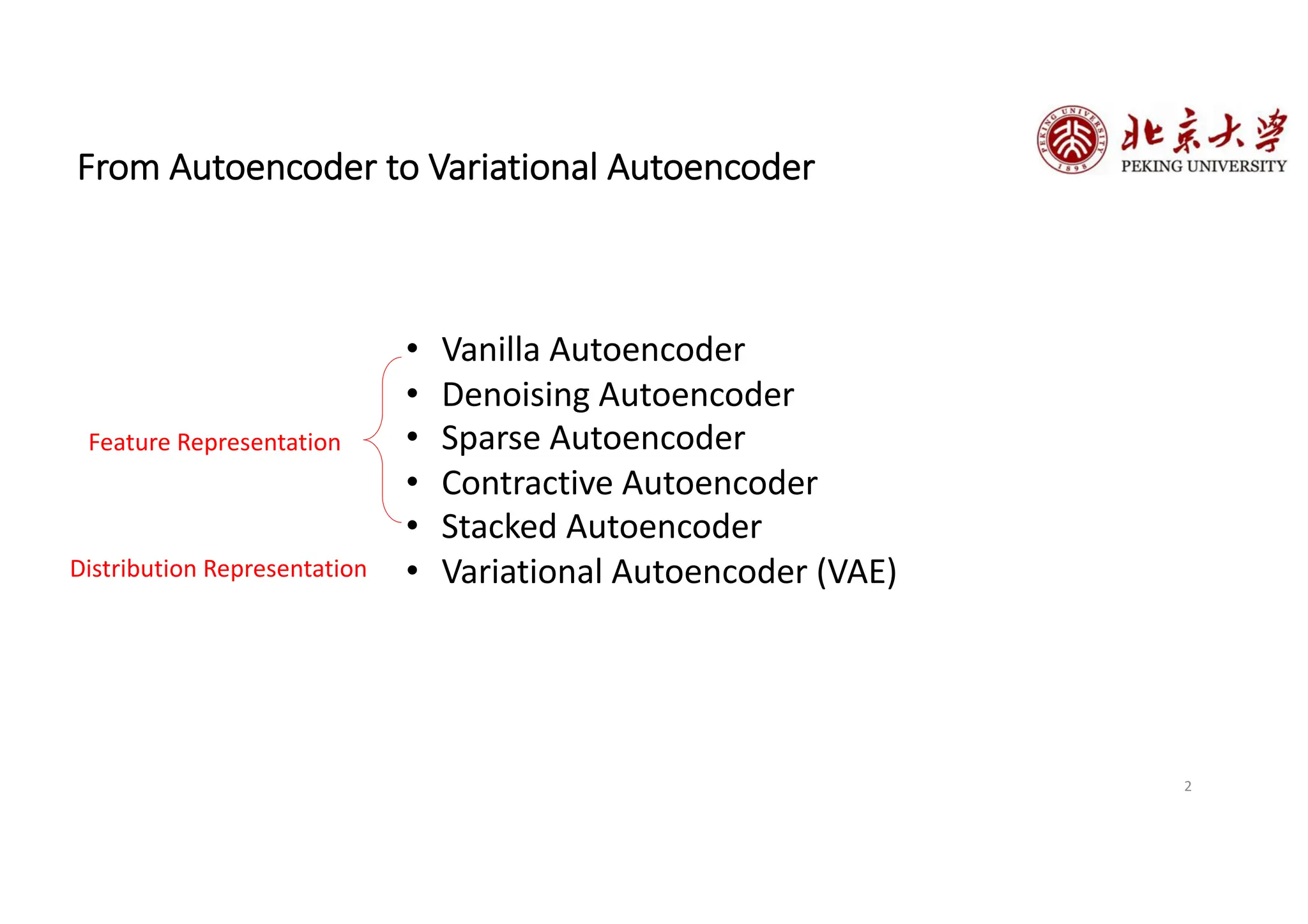
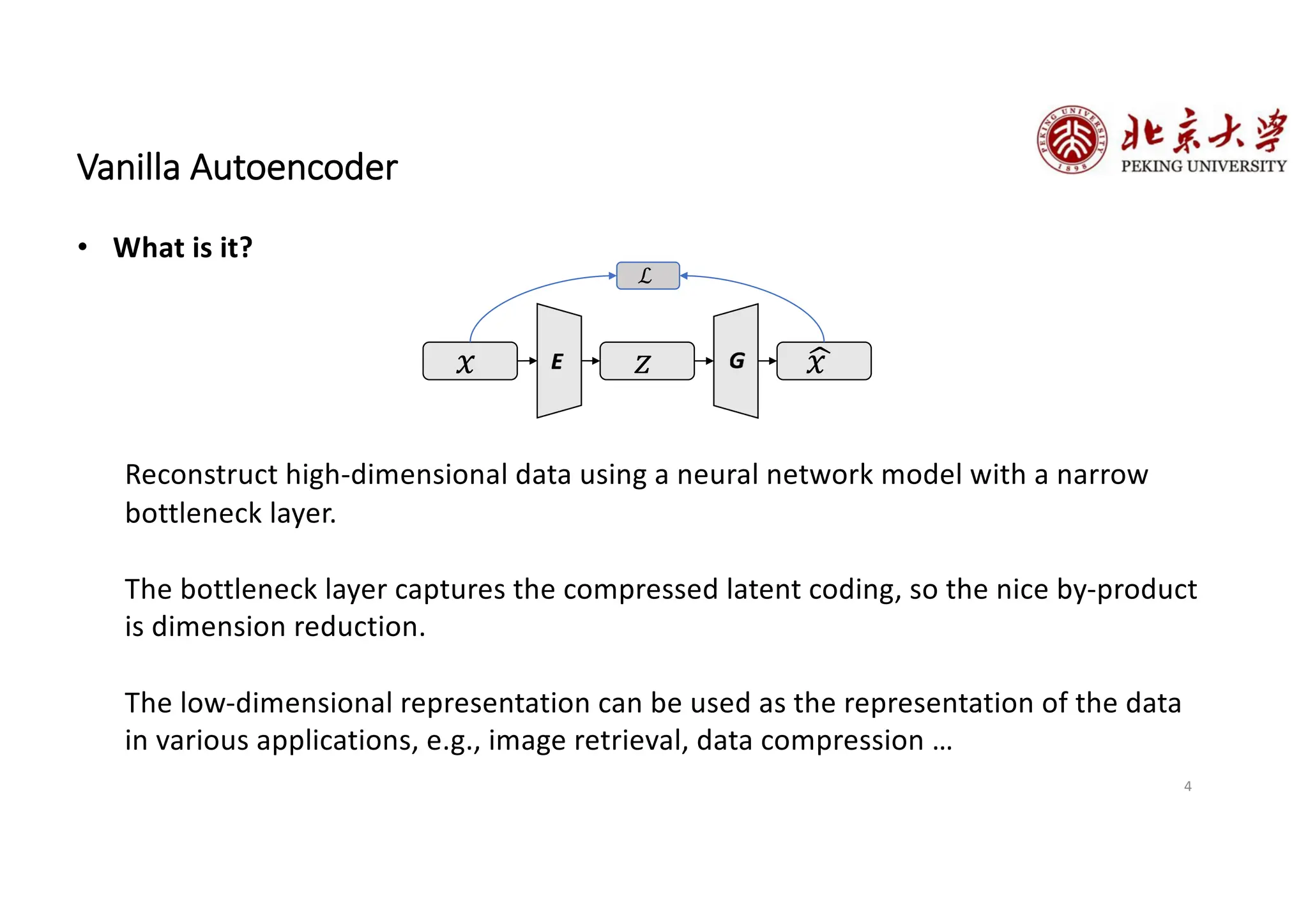
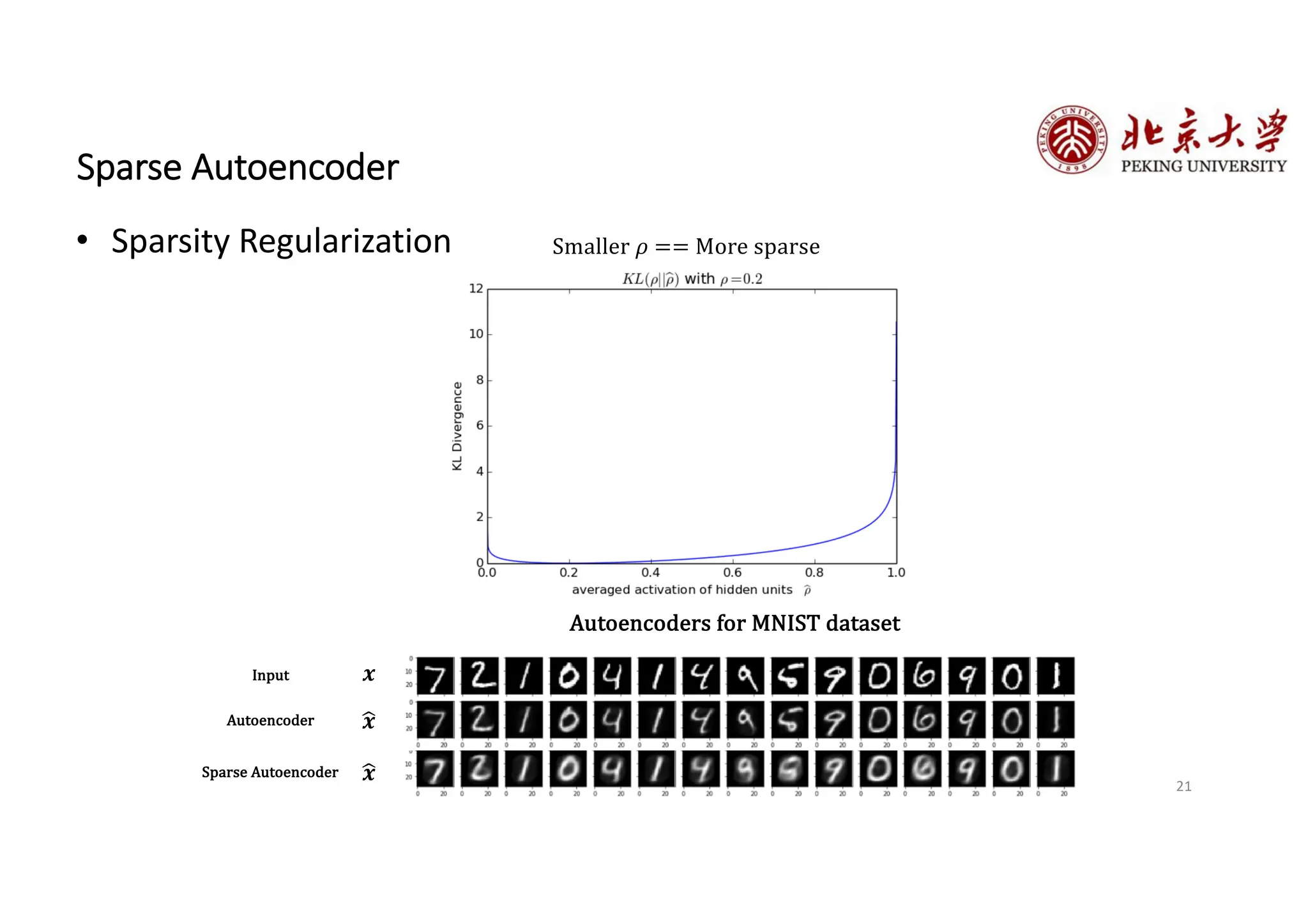
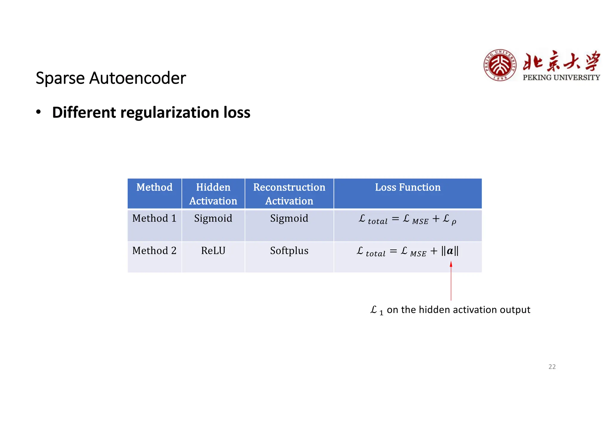
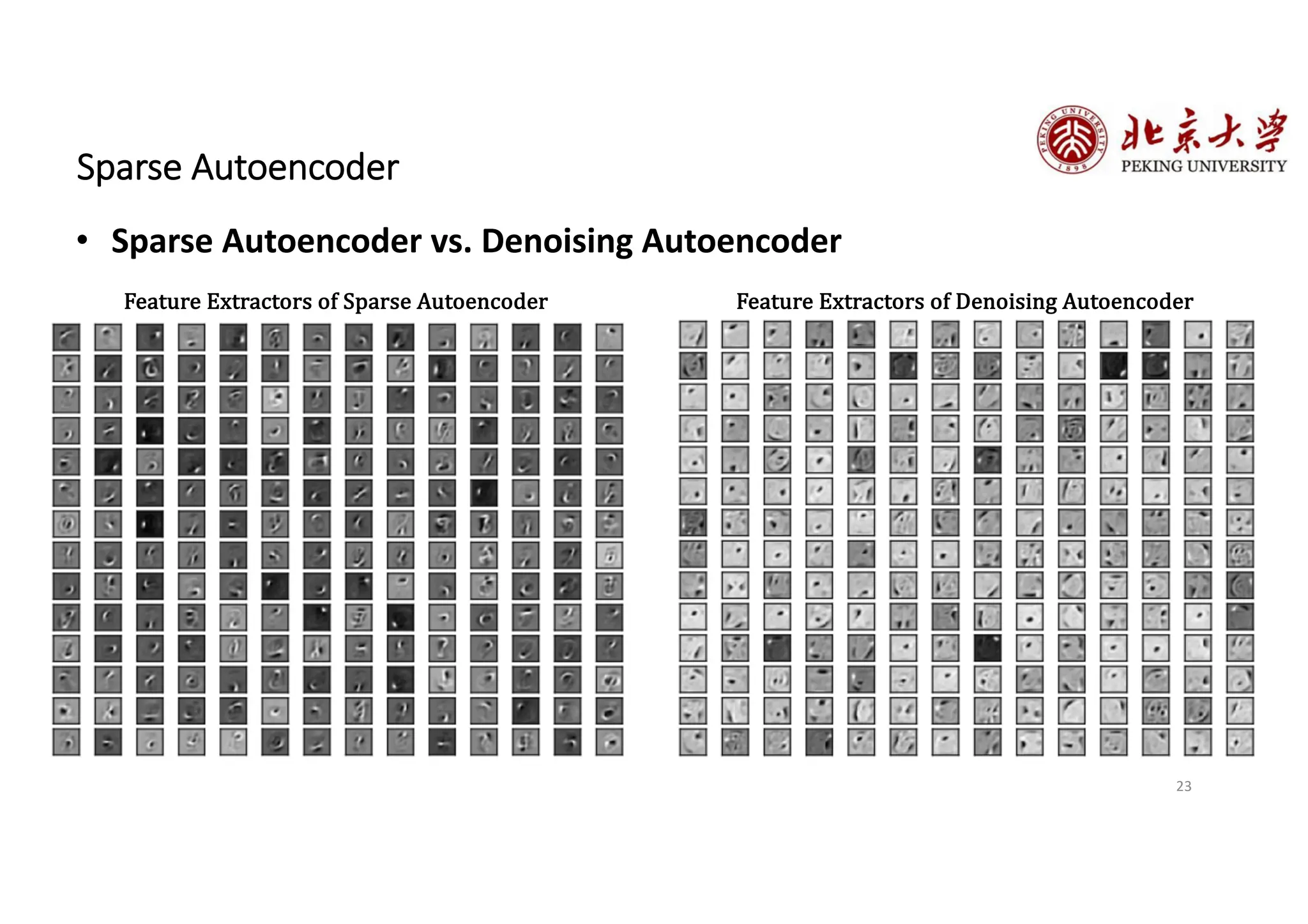
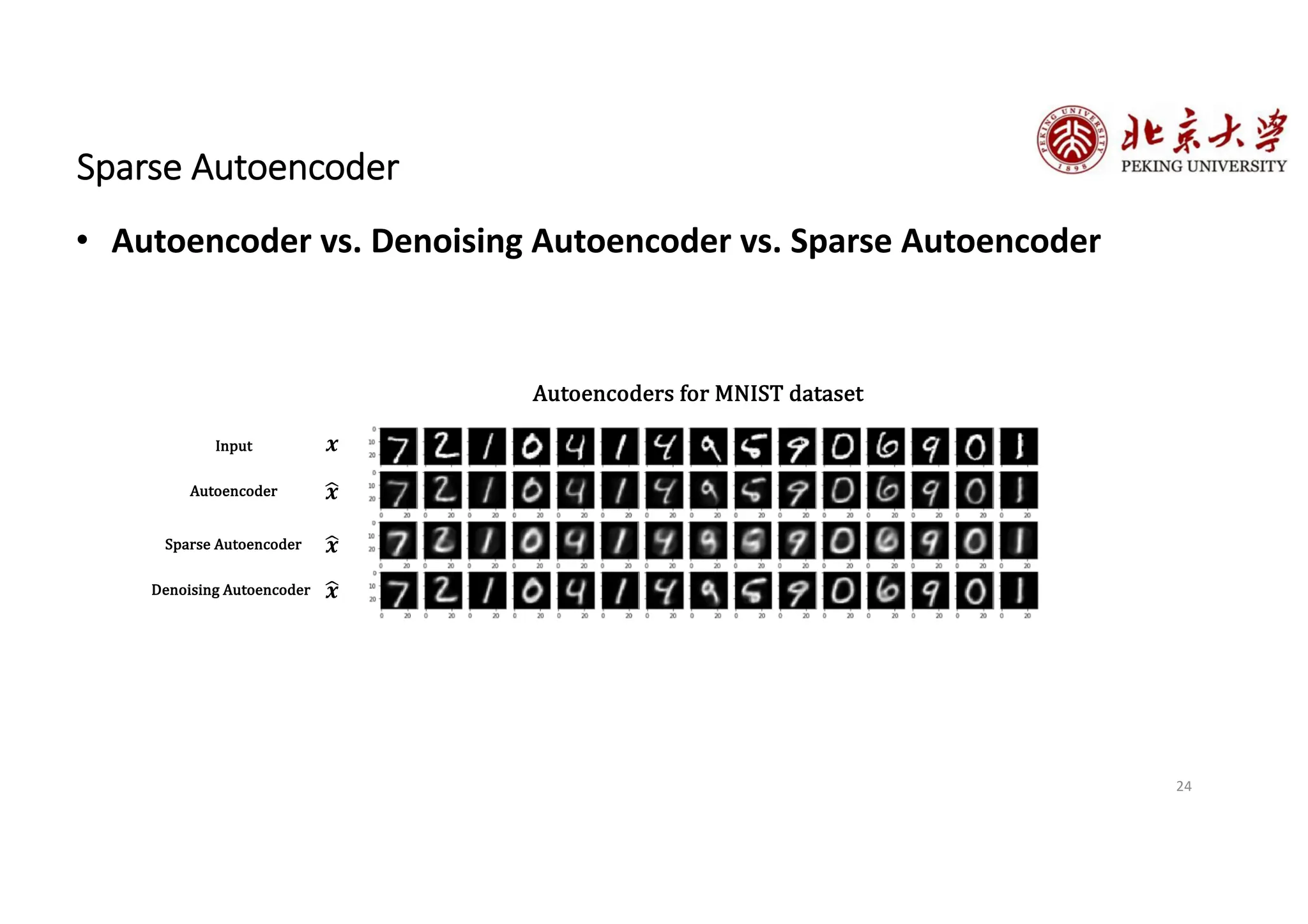
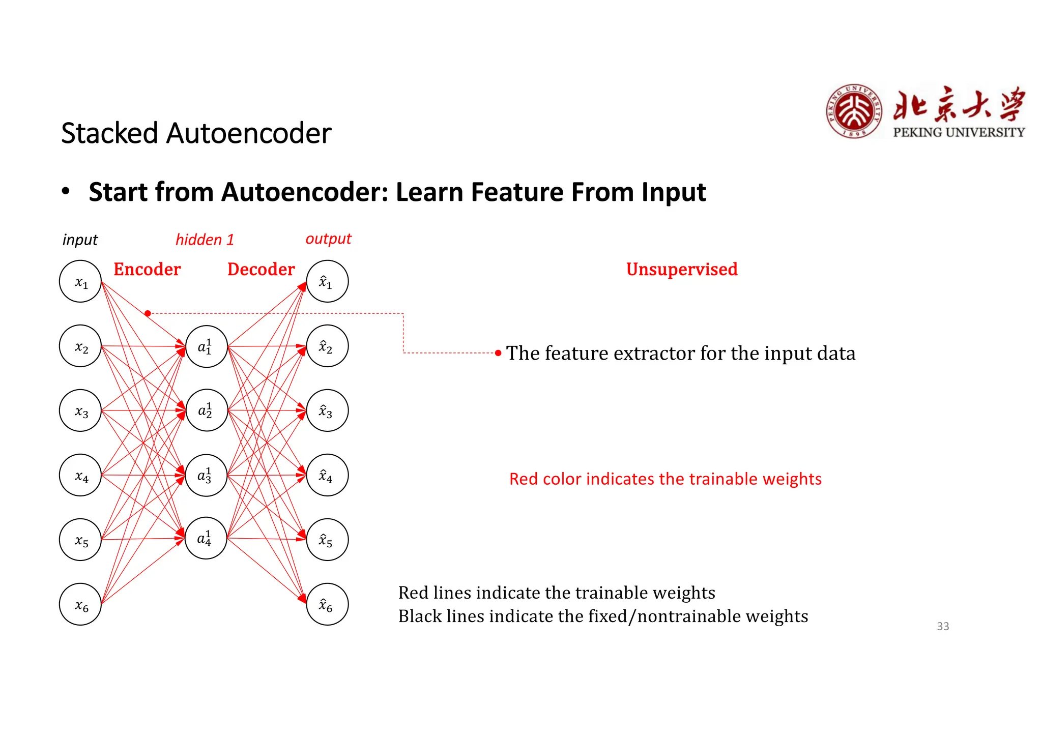
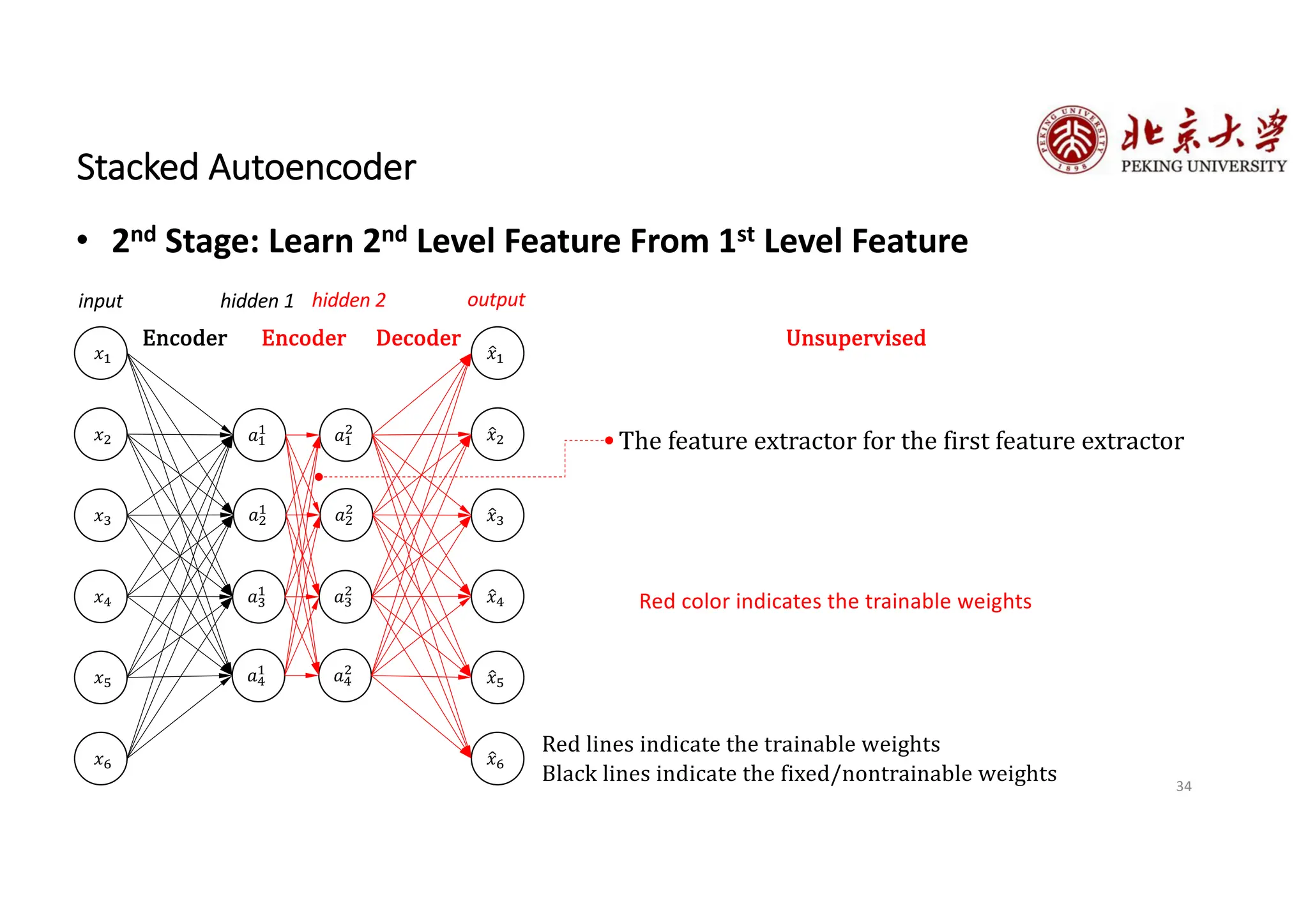
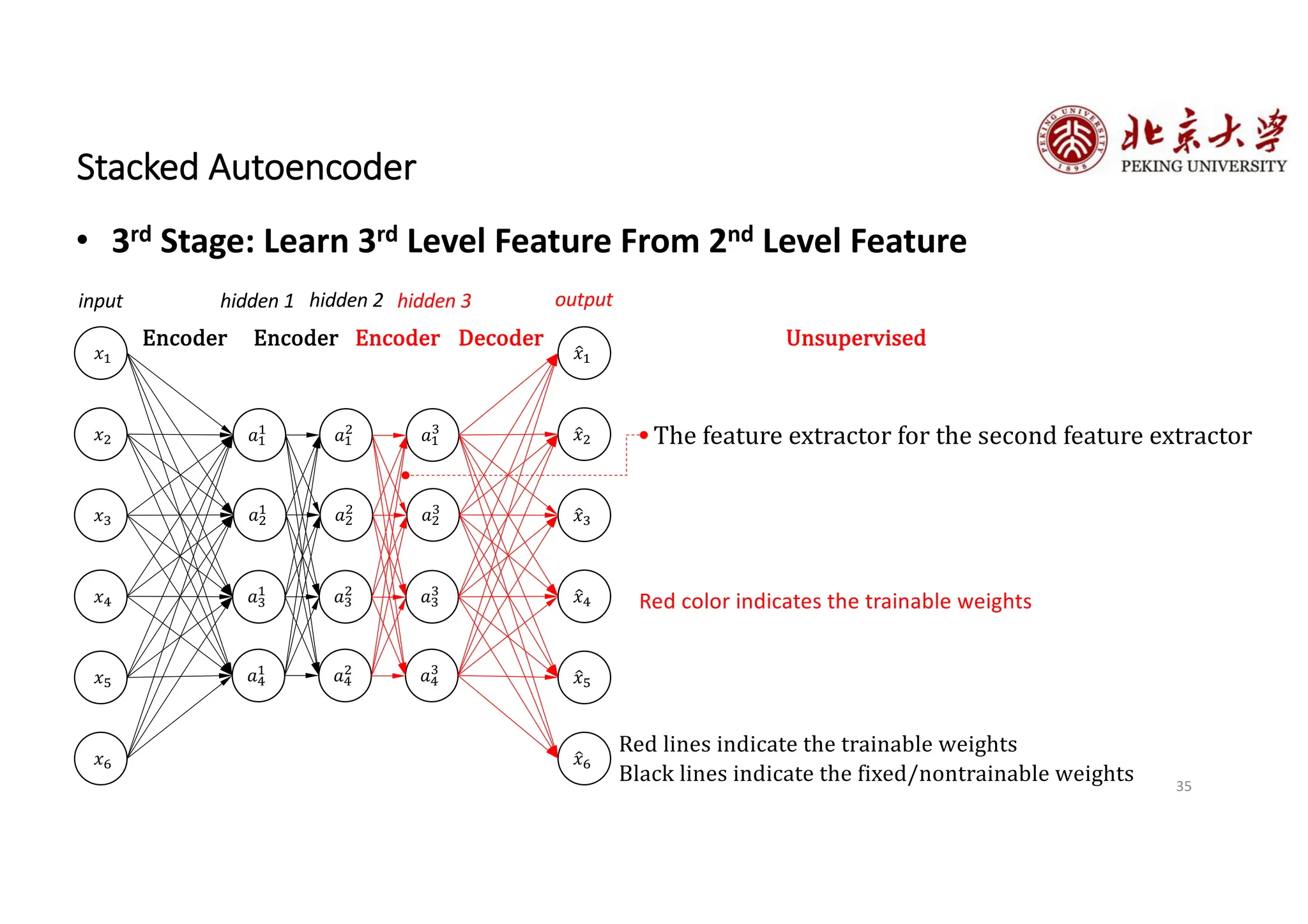
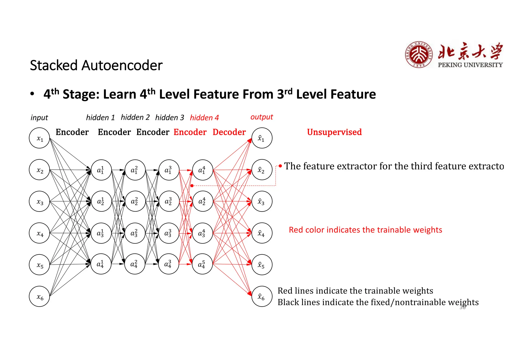
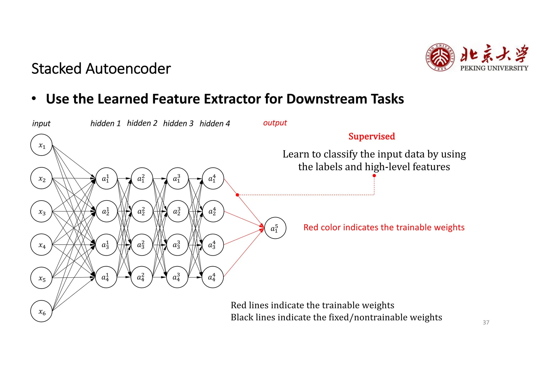
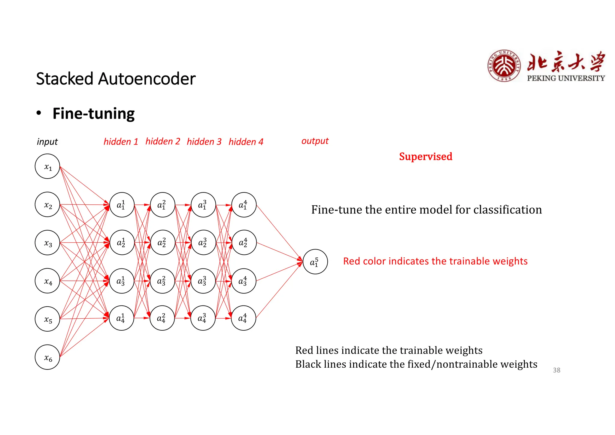
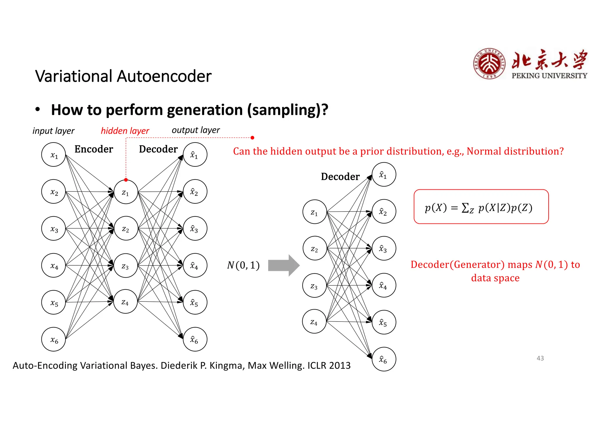
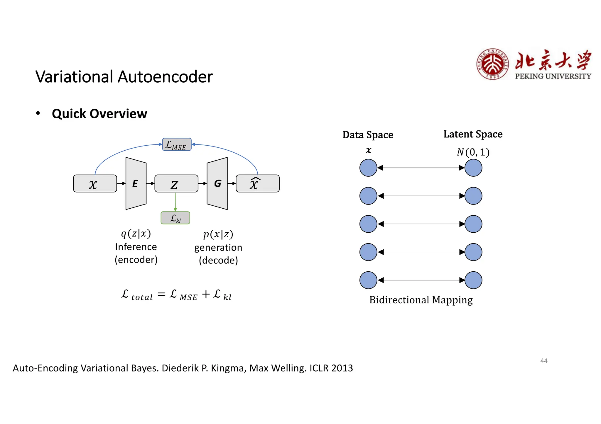
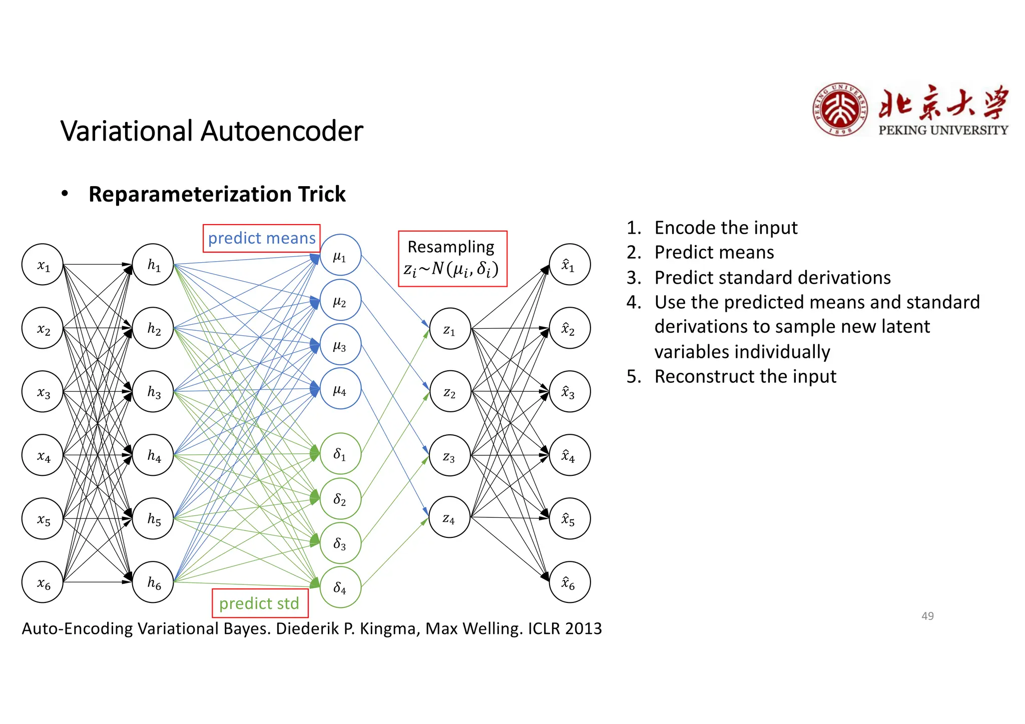
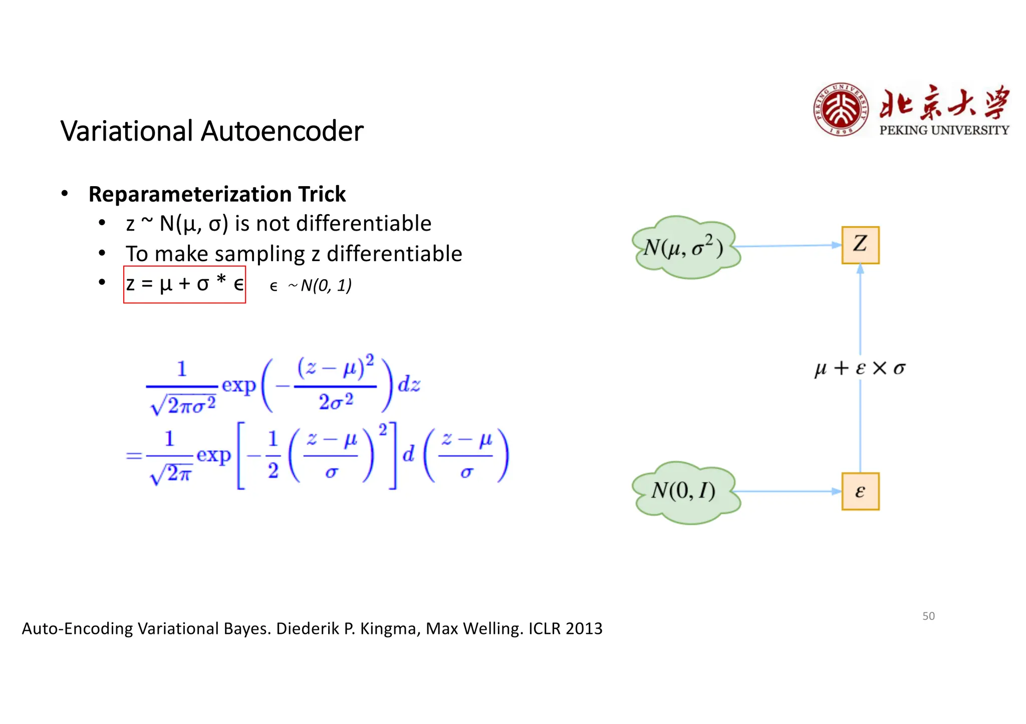
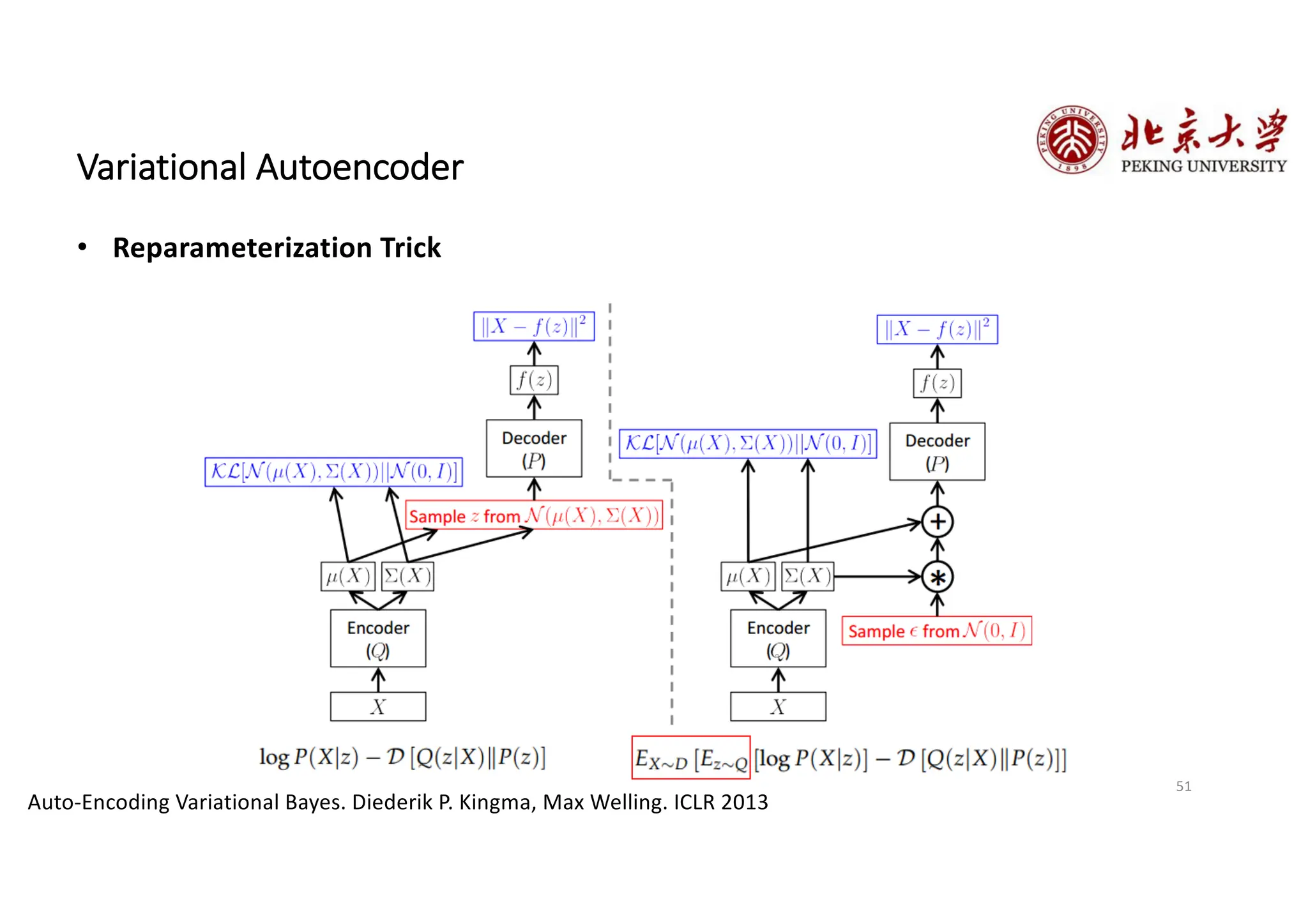
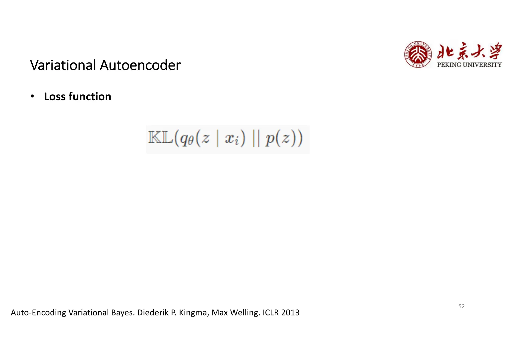
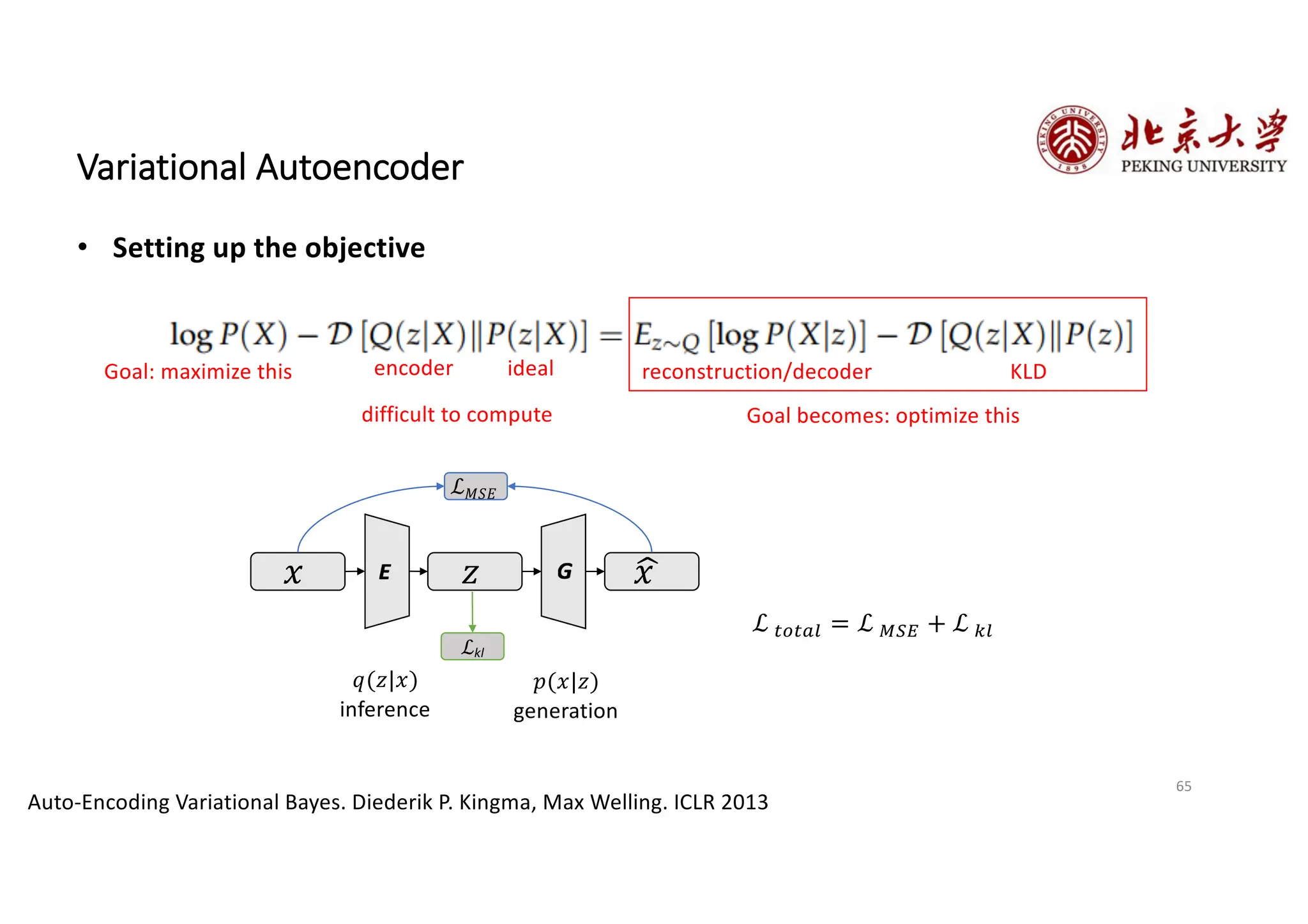
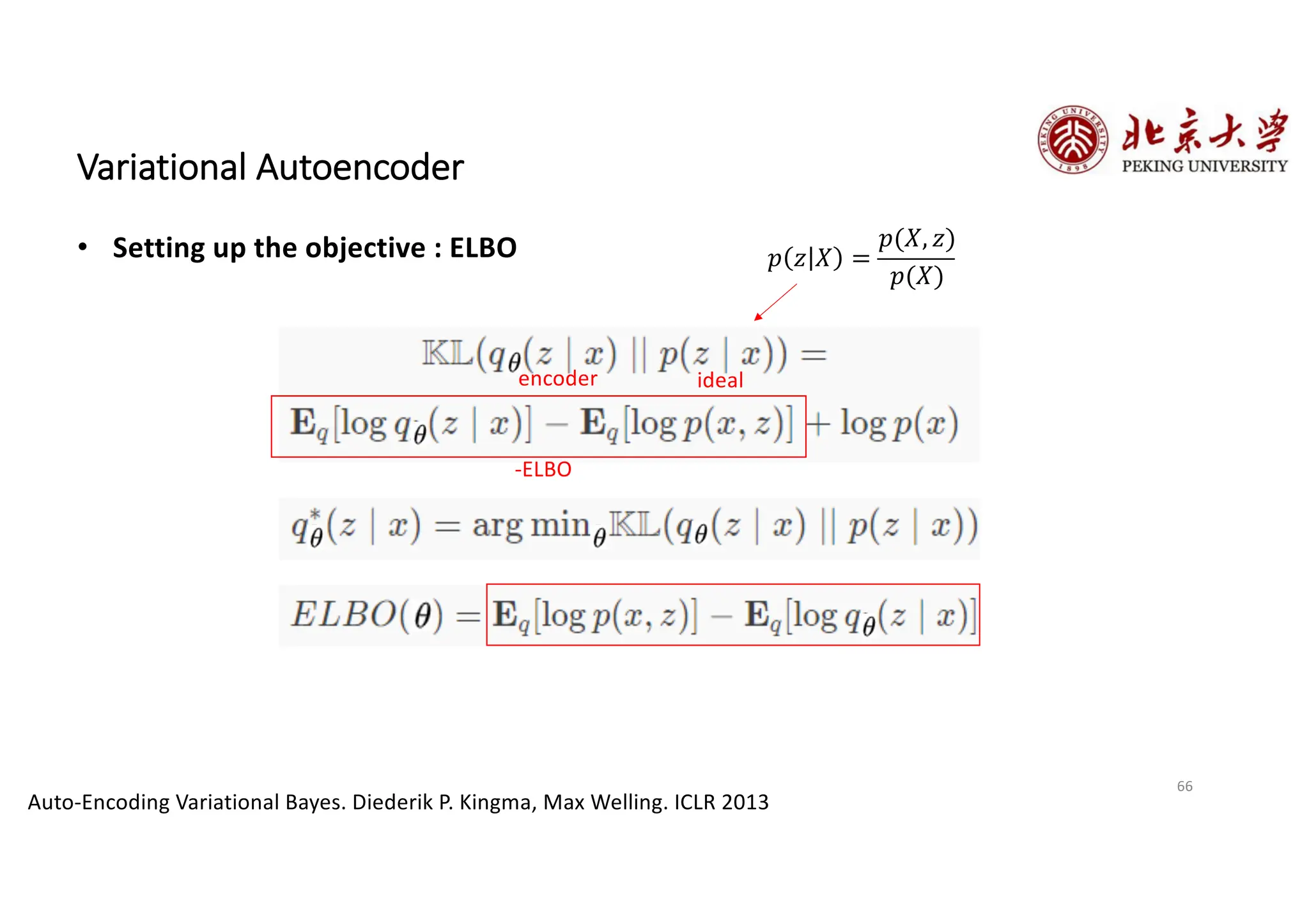
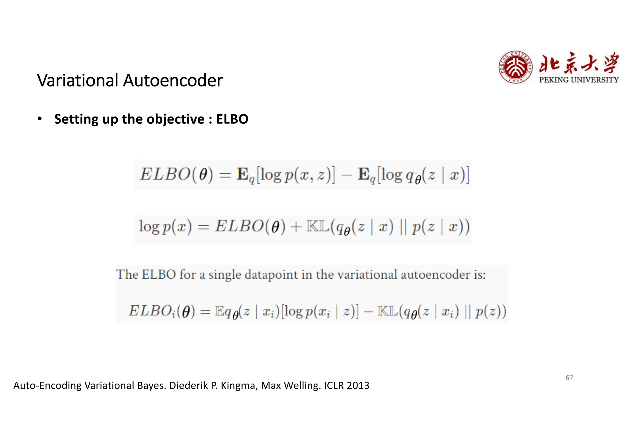
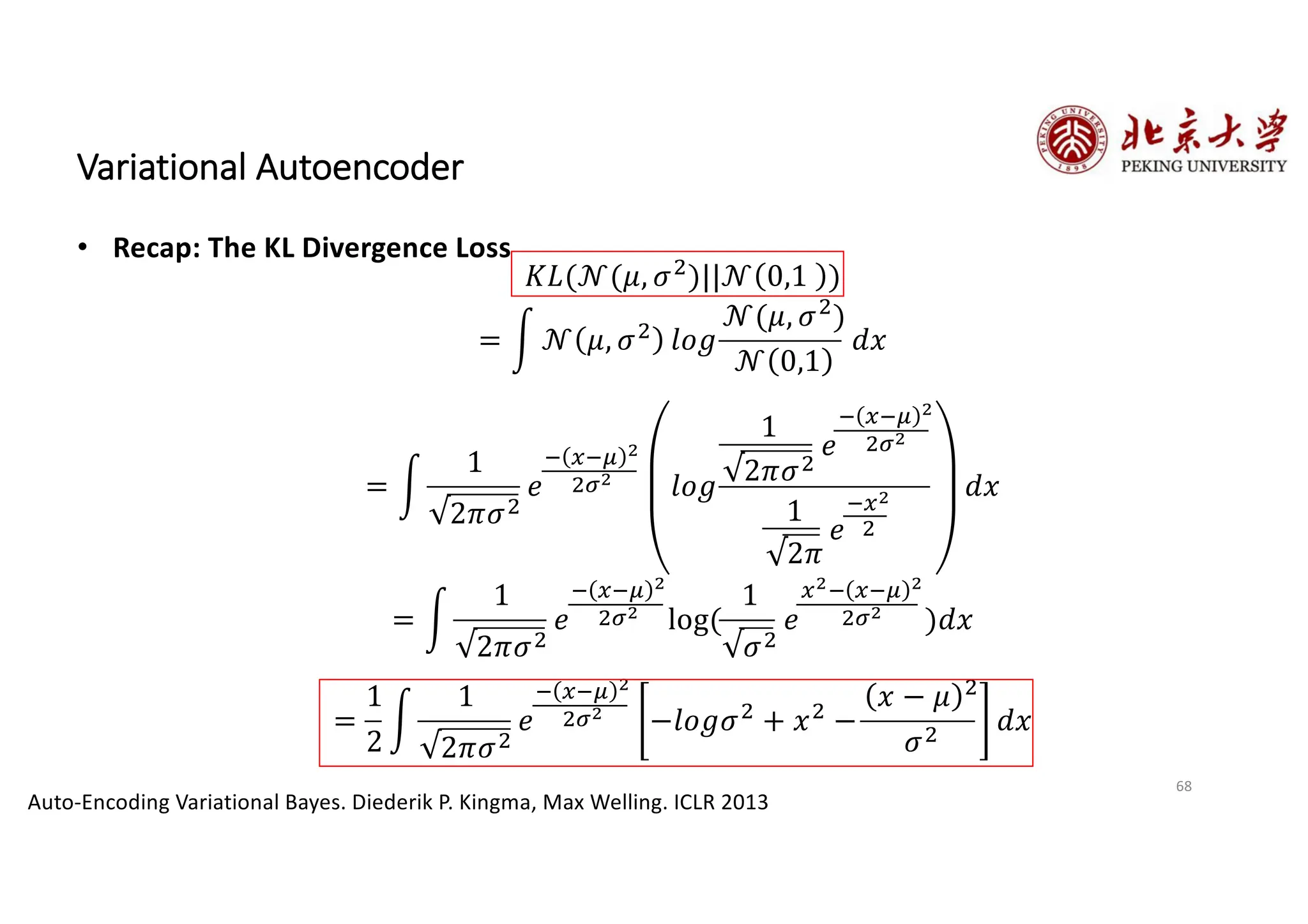
From Autoencoder to Variational Autoencoder Hao Dong Peking University 1
β€’ Vanilla Autoencoder β€’ Denoising Autoencoder β€’ Sparse Autoencoder β€’ Contractive Autoencoder β€’ Stacked Autoencoder β€’ Variational Autoencoder (VAE) 2 From Autoencoder to Variational Autoencoder Feature Representation Distribution Representation θ§†ι’‘οΌšhttps://www.youtube.com/watch
β€’ Vanilla Autoencoder β€’ Denoising Autoencoder β€’ Sparse Autoencoder β€’ Contractive Autoencoder β€’ Stacked Autoencoder β€’ Variational Autoencoder (VAE) 3
4 Vanilla Autoencoder β€’ What is it? Reconstruct high-dimensional data using a neural network model with a narrow bottleneck layer. The bottleneck layer captures the compressed latent coding, so the nice by-product is dimension reduction. The low-dimensional representation can be used as the representation of the data in various applications, e.g., image retrieval, data compression … ! π‘₯ 𝑧 π‘₯ β„’
Latent code: the compressed low dimensional representation of the input data 5 Vanilla Autoencoder β€’ How it works? ! π‘₯ 𝑧 π‘₯ β„’ decoder/generator Z Γ  X encoder X Γ  Z Input Reconstructed Input Ideally the input and reconstruction are identical The encoder network is for dimension reduction, just like PCA
6 Vanilla Autoencoder β€’ Training π‘₯! π‘₯" π‘₯# π‘Ž1 π‘Ž2 π‘Ž3 π‘₯$ π‘₯% π‘₯& π‘Ž4 # π‘₯! # π‘₯" # π‘₯# # π‘₯$ # π‘₯% # π‘₯& hidden layer input layer output layer Given 𝑴 data samples β€’ The hidden units are usually less than the number of inputs β€’ Dimension reduction --- Representation learning The distance between two data can be measure by Mean Squared Error (MSE): β„’ = $ % βˆ‘&'$ % (π‘₯& βˆ’ 𝐺(𝐸 π‘₯& ) 2 where 𝑛 is the number of variables β€’ It is trying to learn an approximation to the identity function so that the input is β€œcompress” to the β€œcompressed” features, discovering interesting structure about the data. Encoder Decoder
7 Vanilla Autoencoder β€’ Testing/Inferencing π‘₯! π‘₯" π‘₯# π‘Ž1 π‘Ž2 π‘Ž3 π‘₯$ π‘₯% π‘₯& π‘Ž4 hidden layer input layer extracted features β€’ Autoencoder is an unsupervised learning method if we considered the latent code as the β€œoutput”. β€’ Autoencoder is also a self-supervised (self-taught) learning method which is a type of supervised learning where the training labels are determined by the input data. β€’ Word2Vec (from RNN lecture) is another unsupervised, self-taught learning example. Autoencoder for MNIST dataset (28Γ—28Γ—1, 784 pixels) % 𝒙 𝒙 Encoder
8 Vanilla Autoencoder β€’ Example: β€’ Compress MNIST (28x28x1) to the latent code with only 2 variables Lossy
9 Vanilla Autoencoder β€’ Power of Latent Representation β€’ t-SNE visualization on MNIST: PCA vs. Autoencoder PCA Autoencoder (Winner) 2006 Science paper by Hinton and Salakhutdinov
10 Vanilla Autoencoder β€’ Discussion β€’ Hidden layer is overcomplete if greater than the input layer
11 Vanilla Autoencoder β€’ Discussion β€’ Hidden layer is overcomplete if greater than the input layer β€’ No compression β€’ No guarantee that the hidden units extract meaningful feature
β€’ Vanilla Autoencoder β€’ Denoising Autoencoder β€’ Sparse Autoencoder β€’ Contractive Autoencoder β€’ Stacked Autoencoder β€’ Variational Autoencoder (VAE) 12
13 Denoising Autoencoder (DAE) β€’ Why? β€’ Avoid overfitting β€’ Learn robust representations
14 Denoising Autoencoder β€’ Architecture π‘₯! π‘₯" π‘₯# π‘Ž1 π‘Ž2 π‘Ž3 π‘₯$ π‘₯% π‘₯& π‘Ž4 # π‘₯! # π‘₯" # π‘₯# # π‘₯$ # π‘₯% # π‘₯& hidden layer input layer output layer π‘₯! π‘₯" π‘₯# π‘₯$ π‘₯% π‘₯& Applying dropout between the input and the first hidden layer β€’ Improve the robustness Encoder Decoder
15 Denoising Autoencoder β€’ Feature Visualization Visualizing the learned features π‘₯! π‘₯" π‘₯# π‘Ž1 π‘Ž2 π‘Ž3 π‘₯$ π‘₯% π‘₯& π‘Ž4 One neuron == One feature extractor reshape Γ 
16 Denoising Autoencoder β€’ Denoising Autoencoder & Dropout Denoising autoencoder was proposed in 2008, 4 years before the dropout paper (Hinton, et al. 2012). Denoising autoencoder can be seem as applying dropout between the input and the first layer. Denoising autoencoder can be seem as one type of data augmentation on the input.
β€’ Vanilla Autoencoder β€’ Denoising Autoencoder β€’ Sparse Autoencoder β€’ Contractive Autoencoder β€’ Stacked Autoencoder β€’ Variational Autoencoder (VAE) 17
18 Sparse Autoencoder β€’ Why? β€’ Even when the number of hidden units is large (perhaps even greater than the number of input pixels), we can still discover interesting structure, by imposing other constraints on the network. β€’ In particular, if we impose a β€β€˜sparsity”’ constraint on the hidden units, then the autoencoder will still discover interesting structure in the data, even if the number of hidden units is large. π‘₯! π‘₯" π‘₯# π‘Ž1 π‘Ž2 π‘Ž3 π‘₯$ π‘₯% π‘₯& π‘Ž4 hidden layer input layer 0.02 β€œinactive” 0.97 β€œactive” 0.01 β€œinactive” 0.98 β€œactive” Sigmoid Encoder
19 Sparse Autoencoder β€’ Recap: KL Divergence Smaller == Closer
20 Sparse Autoencoder β€’ Sparsity Regularization π‘₯! π‘₯" π‘₯# π‘Ž1 π‘Ž2 π‘Ž3 π‘₯$ π‘₯% π‘₯& π‘Ž4 hidden layer input layer 0.02 β€œinactive” 0.97 β€œactive” 0.01 β€œinactive” 0.98 β€œactive” Sigmoid ^ πœŒπ‘— = 1 𝑀 $ "%& ! π‘Žπ‘— Given 𝑴 data samples (batch size) and Sigmoid activation function, the active ratio of a neuron π‘Žπ‘—: To make the output β€œsparse”, we would like to enforce the following constraint, where 𝜌 is a β€œsparsity parameter”, such as 0.2 (20% of the neurons) ^ πœŒπ‘— = 𝜌 The penalty term is as follow, where s is the number of activation outputs. β„’ ' = βˆ‘(%& ) 𝐾𝐿(𝜌|| ^ πœŒπ‘—) = βˆ‘(%& ) (𝜌log ' * '! + (1 βˆ’ 𝜌)log &+' &+* '! ) β„’ ,-,./ = β„’ !01 + πœ†β„’ ' The total loss: Encoder The number of hidden units can be greater than the number of input variables.
21 Sparse Autoencoder β€’ Sparsity Regularization Smaller 𝜌 == More sparse Autoencoders for MNIST dataset % 𝒙 𝒙 Autoencoder Sparse Autoencoder % 𝒙 Input
22 Sparse Autoencoder β€’ Different regularization loss β„’ & on the hidden activation output Method Hidden Activation Reconstruction Activation Loss Function Method 1 Sigmoid Sigmoid β„’ ,-,./ = β„’ !01 + β„’ ' Method 2 ReLU Softplus β„’ ,-,./ = β„’ !01 + 𝒂
23 Sparse Autoencoder β€’ Sparse Autoencoder vs. Denoising Autoencoder Feature Extractors of Sparse Autoencoder Feature Extractors of Denoising Autoencoder
24 Sparse Autoencoder β€’ Autoencoder vs. Denoising Autoencoder vs. Sparse Autoencoder Autoencoders for MNIST dataset % 𝒙 𝒙 Autoencoder Sparse Autoencoder % 𝒙 Input Denoising Autoencoder % 𝒙
β€’ Vanilla Autoencoder β€’ Denoising Autoencoder β€’ Sparse Autoencoder β€’ Contractive Autoencoder β€’ Stacked Autoencoder β€’ Variational Autoencoder (VAE) 25
26 Contractive Autoencoder β€’ Why? β€’ Denoising Autoencoder and Sparse Autoencoder overcome the overcomplete problem via the input and hidden layers. β€’ Could we add an explicit term in the loss to avoid uninteresting features? We wish the features that ONLY reflect variations observed in the training set https://www.youtube.com/watch?v=79sYlJ8Cvlc
27 Contractive Autoencoder β€’ How β€’ Penalize the representation being too sensitive to the input β€’ Improve the robustness to small perturbations β€’ Measure the sensitivity by the Frobenius norm of the Jacobian matrix of the encoder activations
π‘₯ = 𝑓 𝑧 𝑧 = 𝑧! 𝑧" π‘₯ = π‘₯! π‘₯" 𝐽# = ⁄ πœ•π‘₯! πœ•π‘§! ⁄ πœ•π‘₯! πœ•π‘§" ⁄ πœ•π‘₯" πœ•π‘§! ⁄ πœ•π‘₯" πœ•π‘§" 𝐽#!" = ⁄ πœ•π‘§! πœ•π‘₯! ⁄ πœ•π‘§! πœ•π‘₯" ⁄ πœ•π‘§" πœ•π‘₯! ⁄ πœ•π‘§" πœ•π‘₯" 𝑧 = 𝑓$! π‘₯ 𝑧! + 𝑧" 2𝑧! = 𝑓 𝑧! 𝑧" 𝐽# = 1 1 2 0 π‘₯! π‘₯" = π‘₯"/2 π‘₯! βˆ’ π‘₯"/2 = 𝑓$! π‘₯! π‘₯" 𝑧! 𝑧" = 𝐽#!" = 0 1/2 1 βˆ’1/2 input output 𝐽#𝐽#!" = 𝐼 28 Contractive Autoencoder β€’ Recap: Jocobian Matrix
29 Contractive Autoencoder β€’ Jocobian Matrix
30 Contractive Autoencoder β€’ New Loss reconstruction new regularization
31 Contractive Autoencoder β€’ vs. Denoising Autoencoder β€’ Advantages β€’ CAE can better model the distribution of raw data β€’ Disadvantages β€’ DAE is easier to implement β€’ CAE needs second-order optimization (conjugate gradient, LBFGS)
β€’ Vanilla Autoencoder β€’ Denoising Autoencoder β€’ Sparse Autoencoder β€’ Contractive Autoencoder β€’ Stacked Autoencoder β€’ Variational Autoencoder (VAE) 32
33 Stacked Autoencoder β€’ Start from Autoencoder: Learn Feature From Input π‘₯! π‘₯" π‘₯# π‘Ž! ! π‘Ž" ! π‘Ž# ! π‘₯$ π‘₯% π‘₯& π‘Ž$ ! # π‘₯! # π‘₯" # π‘₯# # π‘₯$ # π‘₯% # π‘₯& hidden 1 input output The feature extractor for the input data Red lines indicate the trainable weights Black lines indicate the fixed/nontrainable weights Encoder Decoder Unsupervised Red color indicates the trainable weights
34 Stacked Autoencoder β€’ 2nd Stage: Learn 2nd Level Feature From 1st Level Feature π‘₯! π‘₯" π‘₯# π‘Ž! ! π‘Ž" ! π‘Ž# ! π‘₯$ π‘₯% π‘₯& π‘Ž$ ! hidden 1 input output π‘Ž! " π‘Ž" " π‘Ž# " π‘Ž$ " # π‘₯! # π‘₯" # π‘₯# # π‘₯$ # π‘₯% # π‘₯& hidden 2 The feature extractor for the first feature extractor Red lines indicate the trainable weights Black lines indicate the fixed/nontrainable weights Encoder Encoder Decoder Unsupervised Red color indicates the trainable weights
35 Stacked Autoencoder β€’ 3rd Stage: Learn 3rd Level Feature From 2nd Level Feature π‘₯! π‘₯" π‘₯# π‘Ž! ! π‘Ž" ! π‘Ž# ! π‘₯$ π‘₯% π‘₯& π‘Ž$ ! π‘Ž! " π‘Ž" " π‘Ž# " π‘Ž$ " π‘Ž! # π‘Ž" # π‘Ž# # π‘Ž$ # # π‘₯! # π‘₯" # π‘₯# # π‘₯$ # π‘₯% # π‘₯& hidden 1 input output hidden 2 hidden 3 The feature extractor for the second feature extractor Red lines indicate the trainable weights Black lines indicate the fixed/nontrainable weights Encoder Encoder Encoder Decoder Unsupervised Red color indicates the trainable weights
36 Stacked Autoencoder β€’ 4th Stage: Learn 4th Level Feature From 3rd Level Feature π‘₯! π‘₯" π‘₯# π‘Ž! ! π‘Ž" ! π‘Ž# ! π‘₯$ π‘₯% π‘₯& π‘Ž$ ! π‘Ž! " π‘Ž" " π‘Ž# " π‘Ž$ " π‘Ž! # π‘Ž" # π‘Ž# # π‘Ž$ # hidden 1 input output hidden 2 hidden 3 π‘Ž! $ π‘Ž" $ π‘Ž# $ π‘Ž$ % # π‘₯! # π‘₯" # π‘₯# # π‘₯$ # π‘₯% # π‘₯& hidden 4 The feature extractor for the third feature extractor Red lines indicate the trainable weights Black lines indicate the fixed/nontrainable weights Encoder Encoder Encoder Encoder Decoder Unsupervised Red color indicates the trainable weights
37 Stacked Autoencoder β€’ Use the Learned Feature Extractor for Downstream Tasks π‘₯! π‘₯" π‘₯# π‘Ž! ! π‘Ž" ! π‘Ž# ! π‘₯$ π‘₯% π‘₯& π‘Ž$ ! π‘Ž! " π‘Ž" " π‘Ž# " π‘Ž$ " π‘Ž! # π‘Ž" # π‘Ž# # π‘Ž$ # hidden 1 input output hidden 2 hidden 3 π‘Ž! $ π‘Ž" $ π‘Ž# $ π‘Ž$ $ π‘Ž! % hidden 4 Learn to classify the input data by using the labels and high-level features Red lines indicate the trainable weights Black lines indicate the fixed/nontrainable weights Supervised Red color indicates the trainable weights
38 Stacked Autoencoder β€’ Fine-tuning π‘₯! π‘₯" π‘₯# π‘Ž! ! π‘Ž" ! π‘Ž# ! π‘₯$ π‘₯% π‘₯& π‘Ž$ ! π‘Ž! " π‘Ž" " π‘Ž# " π‘Ž$ " π‘Ž! # π‘Ž" # π‘Ž# # π‘Ž$ # hidden 1 input output hidden 2 hidden 3 π‘Ž! $ π‘Ž" $ π‘Ž# $ π‘Ž$ $ π‘Ž! % hidden 4 Fine-tune the entire model for classification Red lines indicate the trainable weights Black lines indicate the fixed/nontrainable weights Supervised Red color indicates the trainable weights
39 Stacked Autoencoder β€’ Discussion β€’ Advantages β€’ … β€’ Disadvantages β€’ …
β€’ Vanilla Autoencoder β€’ Denoising Autoencoder β€’ Sparse Autoencoder β€’ Contractive Autoencoder β€’ Stacked Autoencoder β€’ Variational Autoencoder (VAE) β€’ From Neural Network Perspective β€’ From Probability Model Perspective 40
41 Before we start β€’ Question? β€’ Are the previous Autoencoders generative model? β€’ Recap: We want to learn a probability distribution 𝑝(π‘₯) over π‘₯ o Generation (sampling): 𝐱pqr~𝑝(x) (NO, The compressed latent codes of autoencoders are not prior distributions, autoencoder cannot learn to represent the data distribution) o Density Estimation: 𝑝(x) high if 𝐱 looks like a real data NO o Unsupervised Representation Learning: Discovering the underlying structure from the data distribution (e.g., ears, nose, eyes …) (YES, Autoencoders learn the feature representation)
β€’ Vanilla Autoencoder β€’ Denoising Autoencoder β€’ Sparse Autoencoder β€’ Contractive Autoencoder β€’ Stacked Autoencoder β€’ Variational Autoencoder (VAE) β€’ From Neural Network Perspective β€’ From Probability Model Perspective 42
43 Variational Autoencoder β€’ How to perform generation (sampling)? π‘₯! π‘₯" π‘₯# 𝑧1 𝑧2 𝑧3 π‘₯$ π‘₯% π‘₯& 𝑧4 # π‘₯! # π‘₯" # π‘₯# # π‘₯$ # π‘₯% # π‘₯& hidden layer input layer output layer Can the hidden output be a prior distribution, e.g., Normal distribution? 𝑧1 𝑧2 𝑧3 𝑧4 # π‘₯! # π‘₯" # π‘₯# # π‘₯$ # π‘₯% # π‘₯& 𝑁(0, 1) Decoder(Generator) maps 𝑁(0, 1) to data space Encoder Decoder Decoder 𝑝 𝑋 = βˆ‘2 𝑝 𝑋 𝑍 𝑝(𝑍) Auto-Encoding Variational Bayes. Diederik P. Kingma, Max Welling. ICLR 2013
44 Variational Autoencoder β€’ Quick Overview β„’kl ! π‘₯ 𝑧 π‘₯ ℒ𝑀𝑆𝐸 𝒙 𝑁(0, 1) Bidirectional Mapping Latent Space Data Space β„’ )*)+, = β„’ -./ + β„’ 0, Auto-Encoding Variational Bayes. Diederik P. Kingma, Max Welling. ICLR 2013 𝑝(π‘₯|𝑧) generation (decode) π‘ž(𝑧|π‘₯) Inference (encoder)
45 Variational Autoencoder β€’ The neural net perspective β€’ A variational autoencoder consists of an encoder, a decoder, and a loss function Auto-Encoding Variational Bayes. Diederik P. Kingma, Max Welling. ICLR 2013
46 Variational Autoencoder β€’ Encoder, Decoder Auto-Encoding Variational Bayes. Diederik P. Kingma, Max Welling. ICLR 2013
47 Variational Autoencoder β€’ Loss function Auto-Encoding Variational Bayes. Diederik P. Kingma, Max Welling. ICLR 2013 regularization Can be represented by MSE
48 β€’ Which direction of the KL divergence to use? β€’ Some applications require an approximation that usually places high probability anywhere that the true distribution places high probability: left one β€’ VAE requires an approximation that rarely places high probability anywhere that the true distribution places low probability: right one Variational Autoencoder β€’ Why KL(Q||P) not KL(P||Q) If:
49 Variational Autoencoder β€’ Reparameterization Trick Auto-Encoding Variational Bayes. Diederik P. Kingma, Max Welling. ICLR 2013 β„Ž! β„Ž" β„Ž# πœ‡1 πœ‡2 πœ‡3 β„Ž$ β„Ž% β„Ž& πœ‡4 # π‘₯! # π‘₯" # π‘₯# # π‘₯$ # π‘₯% # π‘₯& 𝛿1 𝛿2 𝛿3 𝛿4 𝑧1 𝑧2 𝑧3 𝑧4 𝑧3~𝑁(πœ‡3, 𝛿3) Resampling predict means predict std π‘₯! π‘₯" π‘₯# π‘₯$ π‘₯% π‘₯& 1. Encode the input 2. Predict means 3. Predict standard derivations 4. Use the predicted means and standard derivations to sample new latent variables individually 5. Reconstruct the input Latent variables are independent
50 Variational Autoencoder β€’ Reparameterization Trick β€’ z ~ N(ΞΌ, Οƒ) is not differentiable β€’ To make sampling z differentiable β€’ z = ΞΌ + Οƒ * Ο΅ Auto-Encoding Variational Bayes. Diederik P. Kingma, Max Welling. ICLR 2013 Ο΅ ~N(0, 1)
51 Variational Autoencoder β€’ Reparameterization Trick Auto-Encoding Variational Bayes. Diederik P. Kingma, Max Welling. ICLR 2013
52 Variational Autoencoder β€’ Loss function Auto-Encoding Variational Bayes. Diederik P. Kingma, Max Welling. ICLR 2013
53 Variational Autoencoder β€’ Where is β€˜variational’? Auto-Encoding Variational Bayes. Diederik P. Kingma, Max Welling. ICLR 2013
β€’ Vanilla Autoencoder β€’ Denoising Autoencoder β€’ Sparse Autoencoder β€’ Contractive Autoencoder β€’ Stacked Autoencoder β€’ Variational Autoencoder (VAE) β€’ From Neural Network Perspective β€’ From Probability Model Perspective 54
55 Variational Autoencoder β€’ Problem Definition Auto-Encoding Variational Bayes. Diederik P. Kingma, Max Welling. ICLR 2013 Goal: Given 𝑋 = {π‘₯€, π‘₯β€’, π‘₯β€š … , π‘₯p}, find 𝑝 𝑋 to represent 𝑋 How: It is difficult to directly model 𝑝 𝑋 , so alternatively, we can … 𝑝 𝑋 = D Ζ’ 𝑝 𝑋|𝑍 𝑝(𝑍) where 𝑝 𝑍 = 𝑁(0,1) is a prior/known distribution i.e., sample 𝑋 from 𝑍
56 Variational Autoencoder β€’ The probability model perspective β€’ P(X) is hard to model β€’ Alternatively, we learn the joint distribution of X and Z Auto-Encoding Variational Bayes. Diederik P. Kingma, Max Welling. ICLR 2013 𝑝 𝑋 = G 4 𝑝 𝑋|𝑍 𝑝(𝑍) 𝑝 𝑋 = G 4 𝑝 𝑋, 𝑍 𝑝 𝑋, 𝑍 = 𝑝 𝑍 𝑝(𝑋|𝑍)
57 Variational Autoencoder Auto-Encoding Variational Bayes. Diederik P. Kingma, Max Welling. ICLR 2013 β€’ Assumption
58 Variational Autoencoder Auto-Encoding Variational Bayes. Diederik P. Kingma, Max Welling. ICLR 2013 β€’ Assumption
59 Variational Autoencoder Auto-Encoding Variational Bayes. Diederik P. Kingma, Max Welling. ICLR 2013 β€’ Monte Carlo? β€’ n might need to be extremely large before we have an accurate estimation of P(X)
60 Variational Autoencoder Auto-Encoding Variational Bayes. Diederik P. Kingma, Max Welling. ICLR 2013 β€’ Monte Carlo? β€’ Pixel difference is different from perceptual difference
61 Variational Autoencoder Auto-Encoding Variational Bayes. Diederik P. Kingma, Max Welling. ICLR 2013 β€’ Monte Carlo? β€’ VAE alters the sampling procedure
62 Variational Autoencoder Auto-Encoding Variational Bayes. Diederik P. Kingma, Max Welling. ICLR 2013 β€’ Recap: Variational Inference β€’ VI turns inference into optimization ideal approximation 𝑝 𝑧 π‘₯ = 𝑝(π‘₯, 𝑧) 𝑝(π‘₯) ∝ 𝑝(π‘₯, 𝑧)
63 Variational Autoencoder Auto-Encoding Variational Bayes. Diederik P. Kingma, Max Welling. ICLR 2013 β€’ Variational Inference β€’ VI turns inference into optimization parameter distribution
64 Variational Autoencoder Auto-Encoding Variational Bayes. Diederik P. Kingma, Max Welling. ICLR 2013 β€’ Setting up the objective β€’ Maximize P(X) β€’ Set Q(z) to be an arbitrary distribution 𝑝 𝑧 𝑋 = 𝑝 𝑋 𝑧 𝑝(𝑧) 𝑝(𝑋) Goal: maximize this logP(x)
65 Variational Autoencoder Auto-Encoding Variational Bayes. Diederik P. Kingma, Max Welling. ICLR 2013 β€’ Setting up the objective encoder ideal reconstruction/decoder KLD Goal: maximize this Goal becomes: optimize this difficult to compute β„’kl ! π‘₯ 𝑧 π‘₯ ℒ𝑀𝑆𝐸 β„’ )*)+, = β„’ -./ + β„’ 0, 𝑝(π‘₯|𝑧) generation π‘ž(𝑧|π‘₯) inference
66 Variational Autoencoder Auto-Encoding Variational Bayes. Diederik P. Kingma, Max Welling. ICLR 2013 β€’ Setting up the objective : ELBO ideal encoder -ELBO 𝑝 𝑧 𝑋 = 𝑝(𝑋, 𝑧) 𝑝(𝑋)
67 Variational Autoencoder Auto-Encoding Variational Bayes. Diederik P. Kingma, Max Welling. ICLR 2013 β€’ Setting up the objective : ELBO
68 Variational Autoencoder β€’ Recap: The KL Divergence Loss Auto-Encoding Variational Bayes. Diederik P. Kingma, Max Welling. ICLR 2013 𝐾𝐿(𝒩(πœ‡, πœŽβ€’)||𝒩 0,1 ) = O 𝒩 πœ‡, πœŽβ€’ π‘™π‘œπ‘” 𝒩(πœ‡, πœŽβ€’ ) 𝒩 0,1 𝑑π‘₯ = O 1 2πœ‹πœŽβ€’ 𝑒 β€ž β€¦β€žβ€  5 ‒‑5 π‘™π‘œπ‘” 1 2πœ‹πœŽβ€’ 𝑒 β€ž β€¦β€žβ€  5 ‒‑5 1 2πœ‹ 𝑒 β€žβ€¦5 β€’ 𝑑π‘₯ = O 1 2πœ‹πœŽβ€’ 𝑒 β€ž β€¦β€žβ€  5 ‒‑5 log( 1 πœŽβ€’ 𝑒 …5β€ž β€¦β€žβ€  5 ‒‑5 )𝑑π‘₯ = 1 2 O 1 2πœ‹πœŽβ€’ 𝑒 β€ž β€¦β€žβ€  5 ‒‑5 βˆ’π‘™π‘œπ‘”πœŽβ€’ + π‘₯β€’ βˆ’ π‘₯ βˆ’ πœ‡ β€’ πœŽβ€’ 𝑑π‘₯
69 Variational Autoencoder β€’ Recap: The KL Divergence Loss Auto-Encoding Variational Bayes. Diederik P. Kingma, Max Welling. ICLR 2013 𝐾𝐿(𝒩(πœ‡, πœŽβ€’)||𝒩 0,1 ) = 1 2 O 1 2πœ‹πœŽβ€’ 𝑒 β€ž β€¦β€žβ€  5 ‒‑5 βˆ’π‘™π‘œπ‘”πœŽβ€’ + π‘₯β€’ βˆ’ π‘₯ βˆ’ πœ‡ β€’ πœŽβ€’ 𝑑π‘₯ ι‡Š = 1 2 (βˆ’π‘™π‘œπ‘”πœŽ" + πœ‡" + 𝜎" βˆ’ 1)
70 Variational Autoencoder β€’ Recap: The KL Divergence Loss Auto-Encoding Variational Bayes. Diederik P. Kingma, Max Welling. ICLR 2013
71 Variational Autoencoder Auto-Encoding Variational Bayes. Diederik P. Kingma, Max Welling. ICLR 2013 β€’ Optimizing the objective encoder ideal reconstruction KLD dataset dataset
72 Variational Autoencoder β€’ VAE is a Generative Model Auto-Encoding Variational Bayes. Diederik P. Kingma, Max Welling. ICLR 2013 𝑝 𝑍|𝑋 is not 𝑁(0,1) Can we input 𝑁(0,1) to the decoder for sampling? YES: the goal of KL is to make 𝑝 𝑍|𝑋 to be 𝑁(0,1)
73 Variational Autoencoder β€’ VAE vs. Autoencoder β€’ VAE : distribution representation, p(z|x) is a distribution β€’ AE: feature representation, h = E(x) is deterministic Auto-Encoding Variational Bayes. Diederik P. Kingma, Max Welling. ICLR 2013
74 Variational Autoencoder β€’ Challenges β€’ Low quality images β€’ … Auto-Encoding Variational Bayes. Diederik P. Kingma, Max Welling. ICLR 2013
75 Summary: Take Home Message β€’ Autoencoders learn data representation in an unsupervised/ self-supervised way. β€’ Autoencoders learn data representation but cannot model the data distribution 𝑝 𝑋 . β€’ Different with vanilla autoencoder, in sparse autoencoder, the number of hidden units can be greater than the number of input variables. β€’ VAE β€’ … β€’ … β€’ … β€’ … β€’ … β€’ …
Thanks 76

Explanation of Autoencoder to Variontal Auto Encoder

  • 1.
    From Autoencoder toVariational Autoencoder Hao Dong Peking University 1
  • 2.
    β€’ Vanilla Autoencoder β€’Denoising Autoencoder β€’ Sparse Autoencoder β€’ Contractive Autoencoder β€’ Stacked Autoencoder β€’ Variational Autoencoder (VAE) 2 From Autoencoder to Variational Autoencoder Feature Representation Distribution Representation θ§†ι’‘οΌšhttps://www.youtube.com/watch
  • 3.
    β€’ Vanilla Autoencoder β€’Denoising Autoencoder β€’ Sparse Autoencoder β€’ Contractive Autoencoder β€’ Stacked Autoencoder β€’ Variational Autoencoder (VAE) 3
  • 4.
    4 Vanilla Autoencoder β€’ Whatis it? Reconstruct high-dimensional data using a neural network model with a narrow bottleneck layer. The bottleneck layer captures the compressed latent coding, so the nice by-product is dimension reduction. The low-dimensional representation can be used as the representation of the data in various applications, e.g., image retrieval, data compression … ! π‘₯ 𝑧 π‘₯ β„’
  • 5.
    Latent code: thecompressed low dimensional representation of the input data 5 Vanilla Autoencoder β€’ How it works? ! π‘₯ 𝑧 π‘₯ β„’ decoder/generator Z Γ  X encoder X Γ  Z Input Reconstructed Input Ideally the input and reconstruction are identical The encoder network is for dimension reduction, just like PCA
  • 6.
    6 Vanilla Autoencoder β€’ Training π‘₯! π‘₯" π‘₯# π‘Ž1 π‘Ž2 π‘Ž3 π‘₯$ π‘₯% π‘₯& π‘Ž4 # π‘₯! # π‘₯" # π‘₯# # π‘₯$ # π‘₯% # π‘₯& hiddenlayer input layer output layer Given 𝑴 data samples β€’ The hidden units are usually less than the number of inputs β€’ Dimension reduction --- Representation learning The distance between two data can be measure by Mean Squared Error (MSE): β„’ = $ % βˆ‘&'$ % (π‘₯& βˆ’ 𝐺(𝐸 π‘₯& ) 2 where 𝑛 is the number of variables β€’ It is trying to learn an approximation to the identity function so that the input is β€œcompress” to the β€œcompressed” features, discovering interesting structure about the data. Encoder Decoder
  • 7.
    7 Vanilla Autoencoder β€’ Testing/Inferencing π‘₯! π‘₯" π‘₯# π‘Ž1 π‘Ž2 π‘Ž3 π‘₯$ π‘₯% π‘₯& π‘Ž4 hiddenlayer input layer extracted features β€’ Autoencoder is an unsupervised learning method if we considered the latent code as the β€œoutput”. β€’ Autoencoder is also a self-supervised (self-taught) learning method which is a type of supervised learning where the training labels are determined by the input data. β€’ Word2Vec (from RNN lecture) is another unsupervised, self-taught learning example. Autoencoder for MNIST dataset (28Γ—28Γ—1, 784 pixels) % 𝒙 𝒙 Encoder
  • 8.
    8 Vanilla Autoencoder β€’ Example: β€’Compress MNIST (28x28x1) to the latent code with only 2 variables Lossy
  • 9.
    9 Vanilla Autoencoder β€’ Powerof Latent Representation β€’ t-SNE visualization on MNIST: PCA vs. Autoencoder PCA Autoencoder (Winner) 2006 Science paper by Hinton and Salakhutdinov
  • 10.
    10 Vanilla Autoencoder β€’ Discussion β€’Hidden layer is overcomplete if greater than the input layer
  • 11.
    11 Vanilla Autoencoder β€’ Discussion β€’Hidden layer is overcomplete if greater than the input layer β€’ No compression β€’ No guarantee that the hidden units extract meaningful feature
  • 12.
    β€’ Vanilla Autoencoder β€’Denoising Autoencoder β€’ Sparse Autoencoder β€’ Contractive Autoencoder β€’ Stacked Autoencoder β€’ Variational Autoencoder (VAE) 12
  • 13.
    13 Denoising Autoencoder (DAE) β€’Why? β€’ Avoid overfitting β€’ Learn robust representations
  • 14.
    14 Denoising Autoencoder β€’ Architecture π‘₯! π‘₯" π‘₯# π‘Ž1 π‘Ž2 π‘Ž3 π‘₯$ π‘₯% π‘₯& π‘Ž4 # π‘₯! # π‘₯" # π‘₯# # π‘₯$ # π‘₯% # π‘₯& hiddenlayer input layer output layer π‘₯! π‘₯" π‘₯# π‘₯$ π‘₯% π‘₯& Applying dropout between the input and the first hidden layer β€’ Improve the robustness Encoder Decoder
  • 15.
    15 Denoising Autoencoder β€’ FeatureVisualization Visualizing the learned features π‘₯! π‘₯" π‘₯# π‘Ž1 π‘Ž2 π‘Ž3 π‘₯$ π‘₯% π‘₯& π‘Ž4 One neuron == One feature extractor reshape Γ 
  • 16.
    16 Denoising Autoencoder β€’ DenoisingAutoencoder & Dropout Denoising autoencoder was proposed in 2008, 4 years before the dropout paper (Hinton, et al. 2012). Denoising autoencoder can be seem as applying dropout between the input and the first layer. Denoising autoencoder can be seem as one type of data augmentation on the input.
  • 17.
    β€’ Vanilla Autoencoder β€’Denoising Autoencoder β€’ Sparse Autoencoder β€’ Contractive Autoencoder β€’ Stacked Autoencoder β€’ Variational Autoencoder (VAE) 17
  • 18.
    18 Sparse Autoencoder β€’ Why? β€’Even when the number of hidden units is large (perhaps even greater than the number of input pixels), we can still discover interesting structure, by imposing other constraints on the network. β€’ In particular, if we impose a β€β€˜sparsity”’ constraint on the hidden units, then the autoencoder will still discover interesting structure in the data, even if the number of hidden units is large. π‘₯! π‘₯" π‘₯# π‘Ž1 π‘Ž2 π‘Ž3 π‘₯$ π‘₯% π‘₯& π‘Ž4 hidden layer input layer 0.02 β€œinactive” 0.97 β€œactive” 0.01 β€œinactive” 0.98 β€œactive” Sigmoid Encoder
  • 19.
    19 Sparse Autoencoder β€’ Recap:KL Divergence Smaller == Closer
  • 20.
    20 Sparse Autoencoder β€’ SparsityRegularization π‘₯! π‘₯" π‘₯# π‘Ž1 π‘Ž2 π‘Ž3 π‘₯$ π‘₯% π‘₯& π‘Ž4 hidden layer input layer 0.02 β€œinactive” 0.97 β€œactive” 0.01 β€œinactive” 0.98 β€œactive” Sigmoid ^ πœŒπ‘— = 1 𝑀 $ "%& ! π‘Žπ‘— Given 𝑴 data samples (batch size) and Sigmoid activation function, the active ratio of a neuron π‘Žπ‘—: To make the output β€œsparse”, we would like to enforce the following constraint, where 𝜌 is a β€œsparsity parameter”, such as 0.2 (20% of the neurons) ^ πœŒπ‘— = 𝜌 The penalty term is as follow, where s is the number of activation outputs. β„’ ' = βˆ‘(%& ) 𝐾𝐿(𝜌|| ^ πœŒπ‘—) = βˆ‘(%& ) (𝜌log ' * '! + (1 βˆ’ 𝜌)log &+' &+* '! ) β„’ ,-,./ = β„’ !01 + πœ†β„’ ' The total loss: Encoder The number of hidden units can be greater than the number of input variables.
  • 21.
    21 Sparse Autoencoder β€’ SparsityRegularization Smaller 𝜌 == More sparse Autoencoders for MNIST dataset % 𝒙 𝒙 Autoencoder Sparse Autoencoder % 𝒙 Input
  • 22.
    22 Sparse Autoencoder β€’ Differentregularization loss β„’ & on the hidden activation output Method Hidden Activation Reconstruction Activation Loss Function Method 1 Sigmoid Sigmoid β„’ ,-,./ = β„’ !01 + β„’ ' Method 2 ReLU Softplus β„’ ,-,./ = β„’ !01 + 𝒂
  • 23.
    23 Sparse Autoencoder β€’ SparseAutoencoder vs. Denoising Autoencoder Feature Extractors of Sparse Autoencoder Feature Extractors of Denoising Autoencoder
  • 24.
    24 Sparse Autoencoder β€’ Autoencodervs. Denoising Autoencoder vs. Sparse Autoencoder Autoencoders for MNIST dataset % 𝒙 𝒙 Autoencoder Sparse Autoencoder % 𝒙 Input Denoising Autoencoder % 𝒙
  • 25.
    β€’ Vanilla Autoencoder β€’Denoising Autoencoder β€’ Sparse Autoencoder β€’ Contractive Autoencoder β€’ Stacked Autoencoder β€’ Variational Autoencoder (VAE) 25
  • 26.
    26 Contractive Autoencoder β€’ Why? β€’Denoising Autoencoder and Sparse Autoencoder overcome the overcomplete problem via the input and hidden layers. β€’ Could we add an explicit term in the loss to avoid uninteresting features? We wish the features that ONLY reflect variations observed in the training set https://www.youtube.com/watch?v=79sYlJ8Cvlc
  • 27.
    27 Contractive Autoencoder β€’ How β€’Penalize the representation being too sensitive to the input β€’ Improve the robustness to small perturbations β€’ Measure the sensitivity by the Frobenius norm of the Jacobian matrix of the encoder activations
  • 28.
    π‘₯ = 𝑓𝑧 𝑧 = 𝑧! 𝑧" π‘₯ = π‘₯! π‘₯" 𝐽# = ⁄ πœ•π‘₯! πœ•π‘§! ⁄ πœ•π‘₯! πœ•π‘§" ⁄ πœ•π‘₯" πœ•π‘§! ⁄ πœ•π‘₯" πœ•π‘§" 𝐽#!" = ⁄ πœ•π‘§! πœ•π‘₯! ⁄ πœ•π‘§! πœ•π‘₯" ⁄ πœ•π‘§" πœ•π‘₯! ⁄ πœ•π‘§" πœ•π‘₯" 𝑧 = 𝑓$! π‘₯ 𝑧! + 𝑧" 2𝑧! = 𝑓 𝑧! 𝑧" 𝐽# = 1 1 2 0 π‘₯! π‘₯" = π‘₯"/2 π‘₯! βˆ’ π‘₯"/2 = 𝑓$! π‘₯! π‘₯" 𝑧! 𝑧" = 𝐽#!" = 0 1/2 1 βˆ’1/2 input output 𝐽#𝐽#!" = 𝐼 28 Contractive Autoencoder β€’ Recap: Jocobian Matrix
  • 29.
  • 30.
    30 Contractive Autoencoder β€’ NewLoss reconstruction new regularization
  • 31.
    31 Contractive Autoencoder β€’ vs.Denoising Autoencoder β€’ Advantages β€’ CAE can better model the distribution of raw data β€’ Disadvantages β€’ DAE is easier to implement β€’ CAE needs second-order optimization (conjugate gradient, LBFGS)
  • 32.
    β€’ Vanilla Autoencoder β€’Denoising Autoencoder β€’ Sparse Autoencoder β€’ Contractive Autoencoder β€’ Stacked Autoencoder β€’ Variational Autoencoder (VAE) 32
  • 33.
    33 Stacked Autoencoder β€’ Startfrom Autoencoder: Learn Feature From Input π‘₯! π‘₯" π‘₯# π‘Ž! ! π‘Ž" ! π‘Ž# ! π‘₯$ π‘₯% π‘₯& π‘Ž$ ! # π‘₯! # π‘₯" # π‘₯# # π‘₯$ # π‘₯% # π‘₯& hidden 1 input output The feature extractor for the input data Red lines indicate the trainable weights Black lines indicate the fixed/nontrainable weights Encoder Decoder Unsupervised Red color indicates the trainable weights
  • 34.
    34 Stacked Autoencoder β€’ 2ndStage: Learn 2nd Level Feature From 1st Level Feature π‘₯! π‘₯" π‘₯# π‘Ž! ! π‘Ž" ! π‘Ž# ! π‘₯$ π‘₯% π‘₯& π‘Ž$ ! hidden 1 input output π‘Ž! " π‘Ž" " π‘Ž# " π‘Ž$ " # π‘₯! # π‘₯" # π‘₯# # π‘₯$ # π‘₯% # π‘₯& hidden 2 The feature extractor for the first feature extractor Red lines indicate the trainable weights Black lines indicate the fixed/nontrainable weights Encoder Encoder Decoder Unsupervised Red color indicates the trainable weights
  • 35.
    35 Stacked Autoencoder β€’ 3rdStage: Learn 3rd Level Feature From 2nd Level Feature π‘₯! π‘₯" π‘₯# π‘Ž! ! π‘Ž" ! π‘Ž# ! π‘₯$ π‘₯% π‘₯& π‘Ž$ ! π‘Ž! " π‘Ž" " π‘Ž# " π‘Ž$ " π‘Ž! # π‘Ž" # π‘Ž# # π‘Ž$ # # π‘₯! # π‘₯" # π‘₯# # π‘₯$ # π‘₯% # π‘₯& hidden 1 input output hidden 2 hidden 3 The feature extractor for the second feature extractor Red lines indicate the trainable weights Black lines indicate the fixed/nontrainable weights Encoder Encoder Encoder Decoder Unsupervised Red color indicates the trainable weights
  • 36.
    36 Stacked Autoencoder β€’ 4thStage: Learn 4th Level Feature From 3rd Level Feature π‘₯! π‘₯" π‘₯# π‘Ž! ! π‘Ž" ! π‘Ž# ! π‘₯$ π‘₯% π‘₯& π‘Ž$ ! π‘Ž! " π‘Ž" " π‘Ž# " π‘Ž$ " π‘Ž! # π‘Ž" # π‘Ž# # π‘Ž$ # hidden 1 input output hidden 2 hidden 3 π‘Ž! $ π‘Ž" $ π‘Ž# $ π‘Ž$ % # π‘₯! # π‘₯" # π‘₯# # π‘₯$ # π‘₯% # π‘₯& hidden 4 The feature extractor for the third feature extractor Red lines indicate the trainable weights Black lines indicate the fixed/nontrainable weights Encoder Encoder Encoder Encoder Decoder Unsupervised Red color indicates the trainable weights
  • 37.
    37 Stacked Autoencoder β€’ Usethe Learned Feature Extractor for Downstream Tasks π‘₯! π‘₯" π‘₯# π‘Ž! ! π‘Ž" ! π‘Ž# ! π‘₯$ π‘₯% π‘₯& π‘Ž$ ! π‘Ž! " π‘Ž" " π‘Ž# " π‘Ž$ " π‘Ž! # π‘Ž" # π‘Ž# # π‘Ž$ # hidden 1 input output hidden 2 hidden 3 π‘Ž! $ π‘Ž" $ π‘Ž# $ π‘Ž$ $ π‘Ž! % hidden 4 Learn to classify the input data by using the labels and high-level features Red lines indicate the trainable weights Black lines indicate the fixed/nontrainable weights Supervised Red color indicates the trainable weights
  • 38.
    38 Stacked Autoencoder β€’ Fine-tuning π‘₯! π‘₯" π‘₯# π‘Ž! ! π‘Ž" ! π‘Ž# ! π‘₯$ π‘₯% π‘₯& π‘Ž$ ! π‘Ž! " π‘Ž" " π‘Ž# " π‘Ž$ " π‘Ž! # π‘Ž" # π‘Ž# # π‘Ž$ # hidden1 input output hidden 2 hidden 3 π‘Ž! $ π‘Ž" $ π‘Ž# $ π‘Ž$ $ π‘Ž! % hidden 4 Fine-tune the entire model for classification Red lines indicate the trainable weights Black lines indicate the fixed/nontrainable weights Supervised Red color indicates the trainable weights
  • 39.
    39 Stacked Autoencoder β€’ Discussion β€’Advantages β€’ … β€’ Disadvantages β€’ …
  • 40.
    β€’ Vanilla Autoencoder β€’Denoising Autoencoder β€’ Sparse Autoencoder β€’ Contractive Autoencoder β€’ Stacked Autoencoder β€’ Variational Autoencoder (VAE) β€’ From Neural Network Perspective β€’ From Probability Model Perspective 40
  • 41.
    41 Before we start β€’Question? β€’ Are the previous Autoencoders generative model? β€’ Recap: We want to learn a probability distribution 𝑝(π‘₯) over π‘₯ o Generation (sampling): 𝐱pqr~𝑝(x) (NO, The compressed latent codes of autoencoders are not prior distributions, autoencoder cannot learn to represent the data distribution) o Density Estimation: 𝑝(x) high if 𝐱 looks like a real data NO o Unsupervised Representation Learning: Discovering the underlying structure from the data distribution (e.g., ears, nose, eyes …) (YES, Autoencoders learn the feature representation)
  • 42.
    β€’ Vanilla Autoencoder β€’Denoising Autoencoder β€’ Sparse Autoencoder β€’ Contractive Autoencoder β€’ Stacked Autoencoder β€’ Variational Autoencoder (VAE) β€’ From Neural Network Perspective β€’ From Probability Model Perspective 42
  • 43.
    43 Variational Autoencoder β€’ Howto perform generation (sampling)? π‘₯! π‘₯" π‘₯# 𝑧1 𝑧2 𝑧3 π‘₯$ π‘₯% π‘₯& 𝑧4 # π‘₯! # π‘₯" # π‘₯# # π‘₯$ # π‘₯% # π‘₯& hidden layer input layer output layer Can the hidden output be a prior distribution, e.g., Normal distribution? 𝑧1 𝑧2 𝑧3 𝑧4 # π‘₯! # π‘₯" # π‘₯# # π‘₯$ # π‘₯% # π‘₯& 𝑁(0, 1) Decoder(Generator) maps 𝑁(0, 1) to data space Encoder Decoder Decoder 𝑝 𝑋 = βˆ‘2 𝑝 𝑋 𝑍 𝑝(𝑍) Auto-Encoding Variational Bayes. Diederik P. Kingma, Max Welling. ICLR 2013
  • 44.
    44 Variational Autoencoder β€’ QuickOverview β„’kl ! π‘₯ 𝑧 π‘₯ ℒ𝑀𝑆𝐸 𝒙 𝑁(0, 1) Bidirectional Mapping Latent Space Data Space β„’ )*)+, = β„’ -./ + β„’ 0, Auto-Encoding Variational Bayes. Diederik P. Kingma, Max Welling. ICLR 2013 𝑝(π‘₯|𝑧) generation (decode) π‘ž(𝑧|π‘₯) Inference (encoder)
  • 45.
    45 Variational Autoencoder β€’ Theneural net perspective β€’ A variational autoencoder consists of an encoder, a decoder, and a loss function Auto-Encoding Variational Bayes. Diederik P. Kingma, Max Welling. ICLR 2013
  • 46.
    46 Variational Autoencoder β€’ Encoder,Decoder Auto-Encoding Variational Bayes. Diederik P. Kingma, Max Welling. ICLR 2013
  • 47.
    47 Variational Autoencoder β€’ Lossfunction Auto-Encoding Variational Bayes. Diederik P. Kingma, Max Welling. ICLR 2013 regularization Can be represented by MSE
  • 48.
    48 β€’ Which directionof the KL divergence to use? β€’ Some applications require an approximation that usually places high probability anywhere that the true distribution places high probability: left one β€’ VAE requires an approximation that rarely places high probability anywhere that the true distribution places low probability: right one Variational Autoencoder β€’ Why KL(Q||P) not KL(P||Q) If:
  • 49.
    49 Variational Autoencoder β€’ ReparameterizationTrick Auto-Encoding Variational Bayes. Diederik P. Kingma, Max Welling. ICLR 2013 β„Ž! β„Ž" β„Ž# πœ‡1 πœ‡2 πœ‡3 β„Ž$ β„Ž% β„Ž& πœ‡4 # π‘₯! # π‘₯" # π‘₯# # π‘₯$ # π‘₯% # π‘₯& 𝛿1 𝛿2 𝛿3 𝛿4 𝑧1 𝑧2 𝑧3 𝑧4 𝑧3~𝑁(πœ‡3, 𝛿3) Resampling predict means predict std π‘₯! π‘₯" π‘₯# π‘₯$ π‘₯% π‘₯& 1. Encode the input 2. Predict means 3. Predict standard derivations 4. Use the predicted means and standard derivations to sample new latent variables individually 5. Reconstruct the input Latent variables are independent
  • 50.
    50 Variational Autoencoder β€’ ReparameterizationTrick β€’ z ~ N(ΞΌ, Οƒ) is not differentiable β€’ To make sampling z differentiable β€’ z = ΞΌ + Οƒ * Ο΅ Auto-Encoding Variational Bayes. Diederik P. Kingma, Max Welling. ICLR 2013 Ο΅ ~N(0, 1)
  • 51.
    51 Variational Autoencoder β€’ ReparameterizationTrick Auto-Encoding Variational Bayes. Diederik P. Kingma, Max Welling. ICLR 2013
  • 52.
    52 Variational Autoencoder β€’ Lossfunction Auto-Encoding Variational Bayes. Diederik P. Kingma, Max Welling. ICLR 2013
  • 53.
    53 Variational Autoencoder β€’ Whereis β€˜variational’? Auto-Encoding Variational Bayes. Diederik P. Kingma, Max Welling. ICLR 2013
  • 54.
    β€’ Vanilla Autoencoder β€’Denoising Autoencoder β€’ Sparse Autoencoder β€’ Contractive Autoencoder β€’ Stacked Autoencoder β€’ Variational Autoencoder (VAE) β€’ From Neural Network Perspective β€’ From Probability Model Perspective 54
  • 55.
    55 Variational Autoencoder β€’ ProblemDefinition Auto-Encoding Variational Bayes. Diederik P. Kingma, Max Welling. ICLR 2013 Goal: Given 𝑋 = {π‘₯€, π‘₯β€’, π‘₯β€š … , π‘₯p}, find 𝑝 𝑋 to represent 𝑋 How: It is difficult to directly model 𝑝 𝑋 , so alternatively, we can … 𝑝 𝑋 = D Ζ’ 𝑝 𝑋|𝑍 𝑝(𝑍) where 𝑝 𝑍 = 𝑁(0,1) is a prior/known distribution i.e., sample 𝑋 from 𝑍
  • 56.
    56 Variational Autoencoder β€’ Theprobability model perspective β€’ P(X) is hard to model β€’ Alternatively, we learn the joint distribution of X and Z Auto-Encoding Variational Bayes. Diederik P. Kingma, Max Welling. ICLR 2013 𝑝 𝑋 = G 4 𝑝 𝑋|𝑍 𝑝(𝑍) 𝑝 𝑋 = G 4 𝑝 𝑋, 𝑍 𝑝 𝑋, 𝑍 = 𝑝 𝑍 𝑝(𝑋|𝑍)
  • 57.
    57 Variational Autoencoder Auto-Encoding VariationalBayes. Diederik P. Kingma, Max Welling. ICLR 2013 β€’ Assumption
  • 58.
    58 Variational Autoencoder Auto-Encoding VariationalBayes. Diederik P. Kingma, Max Welling. ICLR 2013 β€’ Assumption
  • 59.
    59 Variational Autoencoder Auto-Encoding VariationalBayes. Diederik P. Kingma, Max Welling. ICLR 2013 β€’ Monte Carlo? β€’ n might need to be extremely large before we have an accurate estimation of P(X)
  • 60.
    60 Variational Autoencoder Auto-Encoding VariationalBayes. Diederik P. Kingma, Max Welling. ICLR 2013 β€’ Monte Carlo? β€’ Pixel difference is different from perceptual difference
  • 61.
    61 Variational Autoencoder Auto-Encoding VariationalBayes. Diederik P. Kingma, Max Welling. ICLR 2013 β€’ Monte Carlo? β€’ VAE alters the sampling procedure
  • 62.
    62 Variational Autoencoder Auto-Encoding VariationalBayes. Diederik P. Kingma, Max Welling. ICLR 2013 β€’ Recap: Variational Inference β€’ VI turns inference into optimization ideal approximation 𝑝 𝑧 π‘₯ = 𝑝(π‘₯, 𝑧) 𝑝(π‘₯) ∝ 𝑝(π‘₯, 𝑧)
  • 63.
    63 Variational Autoencoder Auto-Encoding VariationalBayes. Diederik P. Kingma, Max Welling. ICLR 2013 β€’ Variational Inference β€’ VI turns inference into optimization parameter distribution
  • 64.
    64 Variational Autoencoder Auto-Encoding VariationalBayes. Diederik P. Kingma, Max Welling. ICLR 2013 β€’ Setting up the objective β€’ Maximize P(X) β€’ Set Q(z) to be an arbitrary distribution 𝑝 𝑧 𝑋 = 𝑝 𝑋 𝑧 𝑝(𝑧) 𝑝(𝑋) Goal: maximize this logP(x)
  • 65.
    65 Variational Autoencoder Auto-Encoding VariationalBayes. Diederik P. Kingma, Max Welling. ICLR 2013 β€’ Setting up the objective encoder ideal reconstruction/decoder KLD Goal: maximize this Goal becomes: optimize this difficult to compute β„’kl ! π‘₯ 𝑧 π‘₯ ℒ𝑀𝑆𝐸 β„’ )*)+, = β„’ -./ + β„’ 0, 𝑝(π‘₯|𝑧) generation π‘ž(𝑧|π‘₯) inference
  • 66.
    66 Variational Autoencoder Auto-Encoding VariationalBayes. Diederik P. Kingma, Max Welling. ICLR 2013 β€’ Setting up the objective : ELBO ideal encoder -ELBO 𝑝 𝑧 𝑋 = 𝑝(𝑋, 𝑧) 𝑝(𝑋)
  • 67.
    67 Variational Autoencoder Auto-Encoding VariationalBayes. Diederik P. Kingma, Max Welling. ICLR 2013 β€’ Setting up the objective : ELBO
  • 68.
    68 Variational Autoencoder β€’ Recap:The KL Divergence Loss Auto-Encoding Variational Bayes. Diederik P. Kingma, Max Welling. ICLR 2013 𝐾𝐿(𝒩(πœ‡, πœŽβ€’)||𝒩 0,1 ) = O 𝒩 πœ‡, πœŽβ€’ π‘™π‘œπ‘” 𝒩(πœ‡, πœŽβ€’ ) 𝒩 0,1 𝑑π‘₯ = O 1 2πœ‹πœŽβ€’ 𝑒 β€ž β€¦β€žβ€  5 ‒‑5 π‘™π‘œπ‘” 1 2πœ‹πœŽβ€’ 𝑒 β€ž β€¦β€žβ€  5 ‒‑5 1 2πœ‹ 𝑒 β€žβ€¦5 β€’ 𝑑π‘₯ = O 1 2πœ‹πœŽβ€’ 𝑒 β€ž β€¦β€žβ€  5 ‒‑5 log( 1 πœŽβ€’ 𝑒 …5β€ž β€¦β€žβ€  5 ‒‑5 )𝑑π‘₯ = 1 2 O 1 2πœ‹πœŽβ€’ 𝑒 β€ž β€¦β€žβ€  5 ‒‑5 βˆ’π‘™π‘œπ‘”πœŽβ€’ + π‘₯β€’ βˆ’ π‘₯ βˆ’ πœ‡ β€’ πœŽβ€’ 𝑑π‘₯
  • 69.
    69 Variational Autoencoder β€’ Recap:The KL Divergence Loss Auto-Encoding Variational Bayes. Diederik P. Kingma, Max Welling. ICLR 2013 𝐾𝐿(𝒩(πœ‡, πœŽβ€’)||𝒩 0,1 ) = 1 2 O 1 2πœ‹πœŽβ€’ 𝑒 β€ž β€¦β€žβ€  5 ‒‑5 βˆ’π‘™π‘œπ‘”πœŽβ€’ + π‘₯β€’ βˆ’ π‘₯ βˆ’ πœ‡ β€’ πœŽβ€’ 𝑑π‘₯ ι‡Š = 1 2 (βˆ’π‘™π‘œπ‘”πœŽ" + πœ‡" + 𝜎" βˆ’ 1)
  • 70.
    70 Variational Autoencoder β€’ Recap:The KL Divergence Loss Auto-Encoding Variational Bayes. Diederik P. Kingma, Max Welling. ICLR 2013
  • 71.
    71 Variational Autoencoder Auto-Encoding VariationalBayes. Diederik P. Kingma, Max Welling. ICLR 2013 β€’ Optimizing the objective encoder ideal reconstruction KLD dataset dataset
  • 72.
    72 Variational Autoencoder β€’ VAEis a Generative Model Auto-Encoding Variational Bayes. Diederik P. Kingma, Max Welling. ICLR 2013 𝑝 𝑍|𝑋 is not 𝑁(0,1) Can we input 𝑁(0,1) to the decoder for sampling? YES: the goal of KL is to make 𝑝 𝑍|𝑋 to be 𝑁(0,1)
  • 73.
    73 Variational Autoencoder β€’ VAEvs. Autoencoder β€’ VAE : distribution representation, p(z|x) is a distribution β€’ AE: feature representation, h = E(x) is deterministic Auto-Encoding Variational Bayes. Diederik P. Kingma, Max Welling. ICLR 2013
  • 74.
    74 Variational Autoencoder β€’ Challenges β€’Low quality images β€’ … Auto-Encoding Variational Bayes. Diederik P. Kingma, Max Welling. ICLR 2013
  • 75.
    75 Summary: Take HomeMessage β€’ Autoencoders learn data representation in an unsupervised/ self-supervised way. β€’ Autoencoders learn data representation but cannot model the data distribution 𝑝 𝑋 . β€’ Different with vanilla autoencoder, in sparse autoencoder, the number of hidden units can be greater than the number of input variables. β€’ VAE β€’ … β€’ … β€’ … β€’ … β€’ … β€’ …
  • 76.