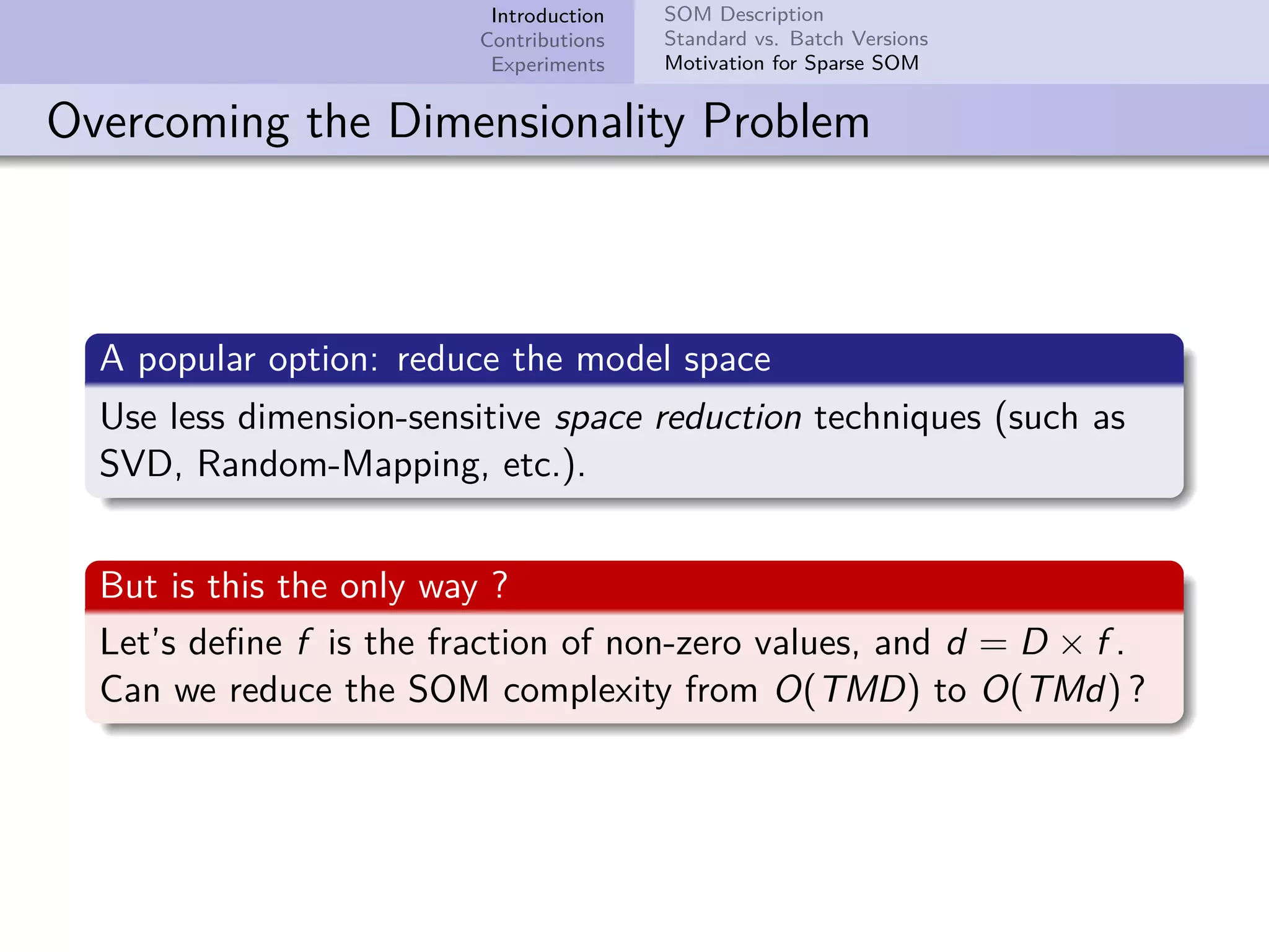
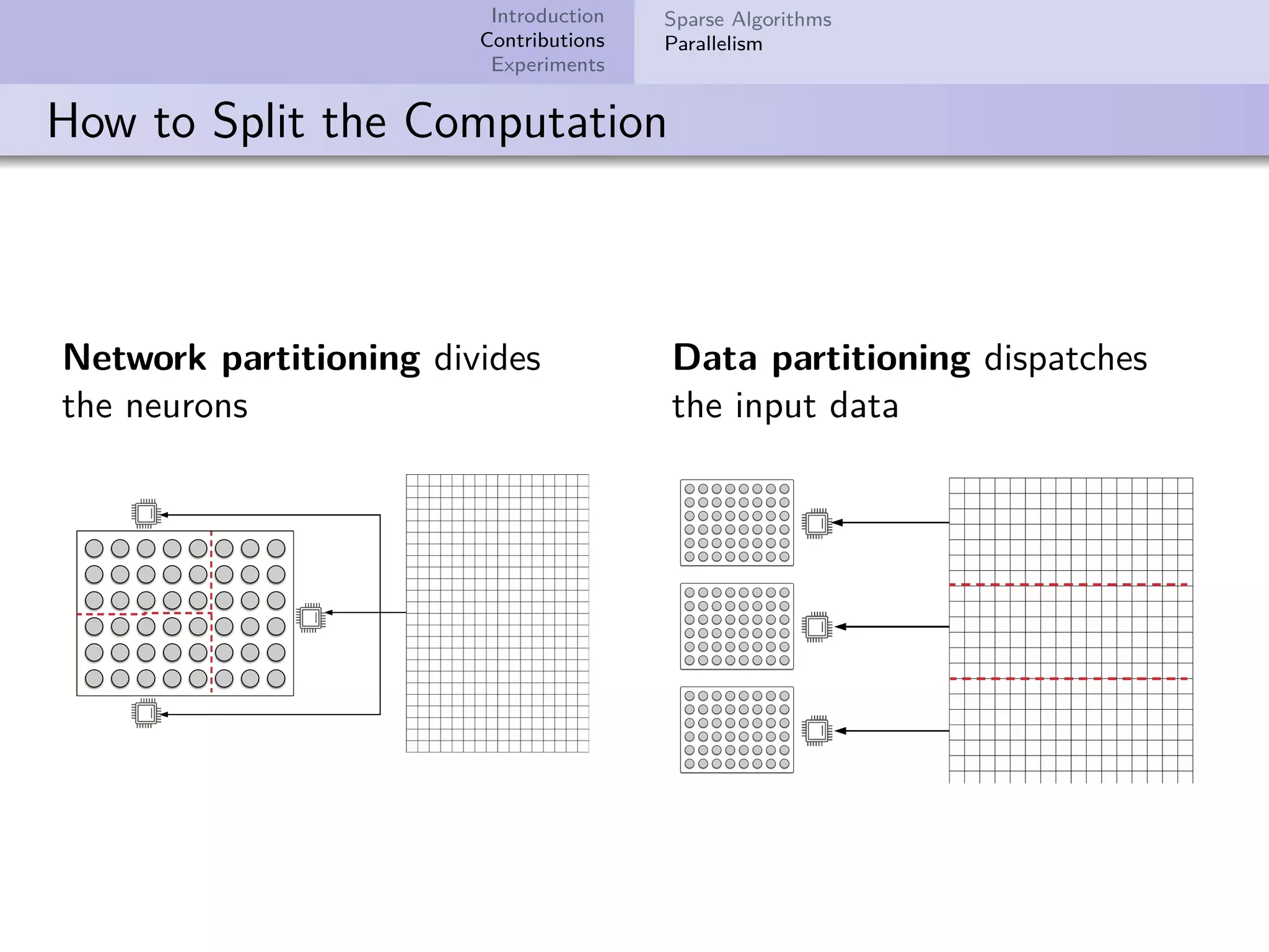
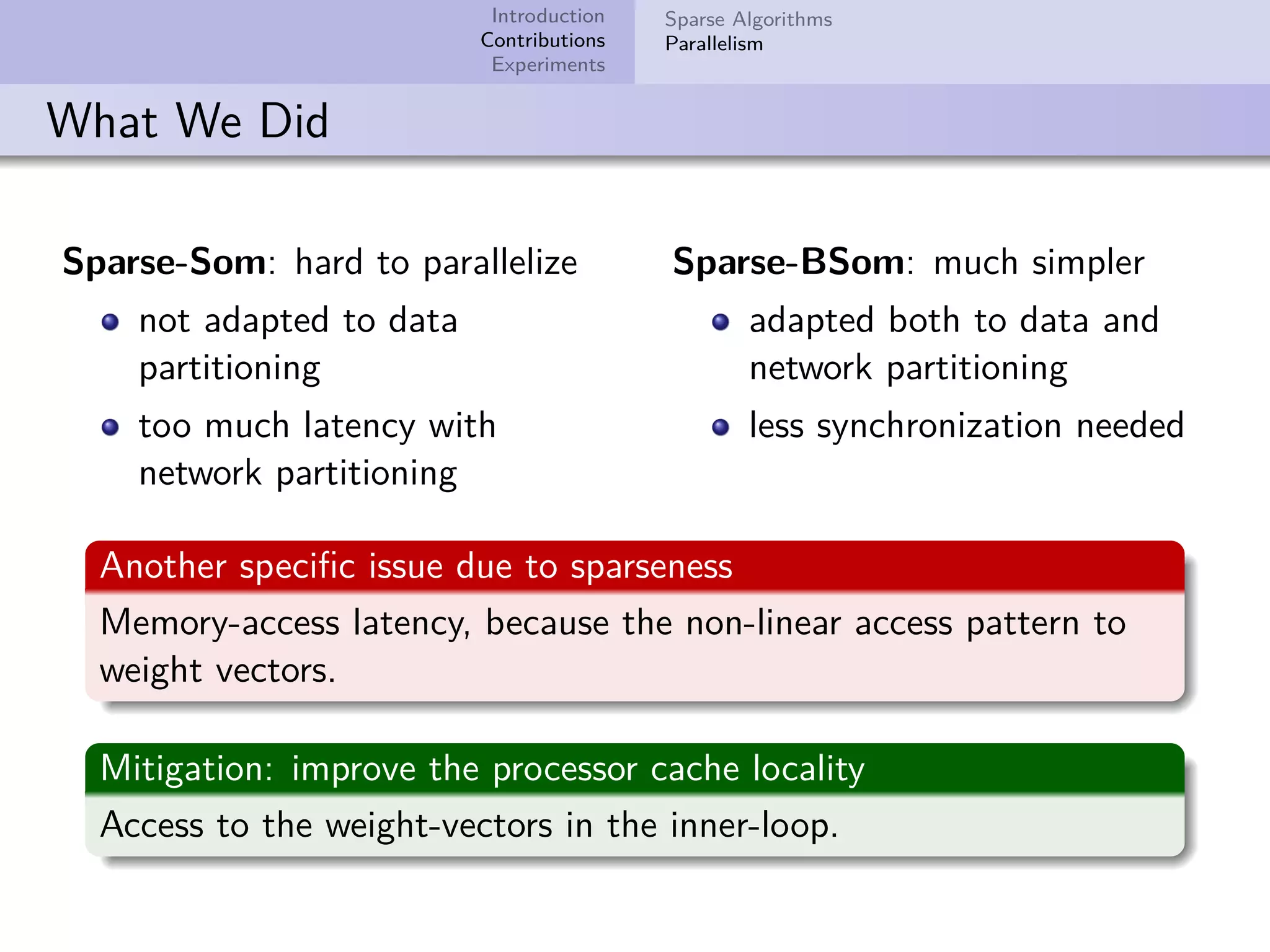
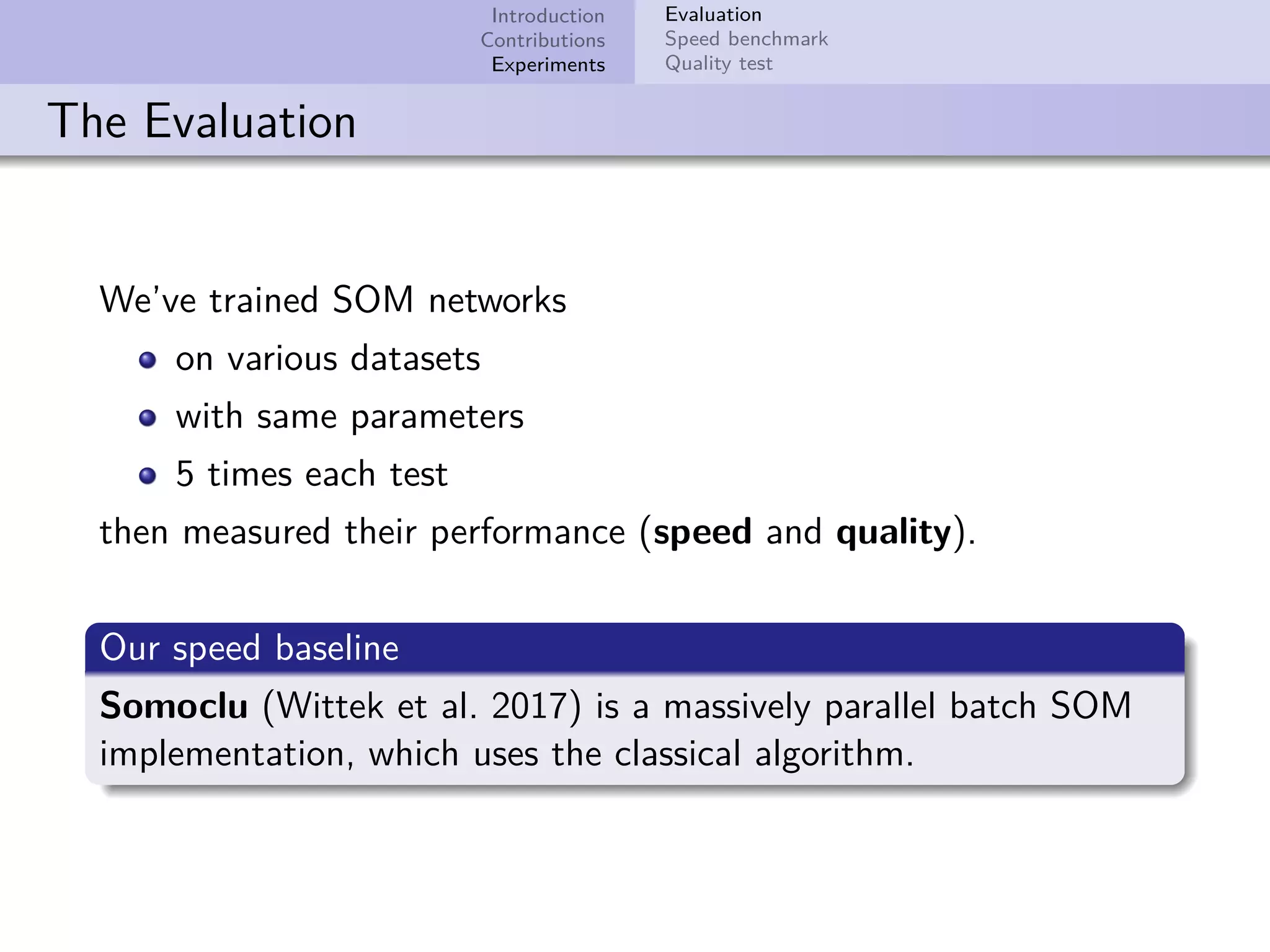
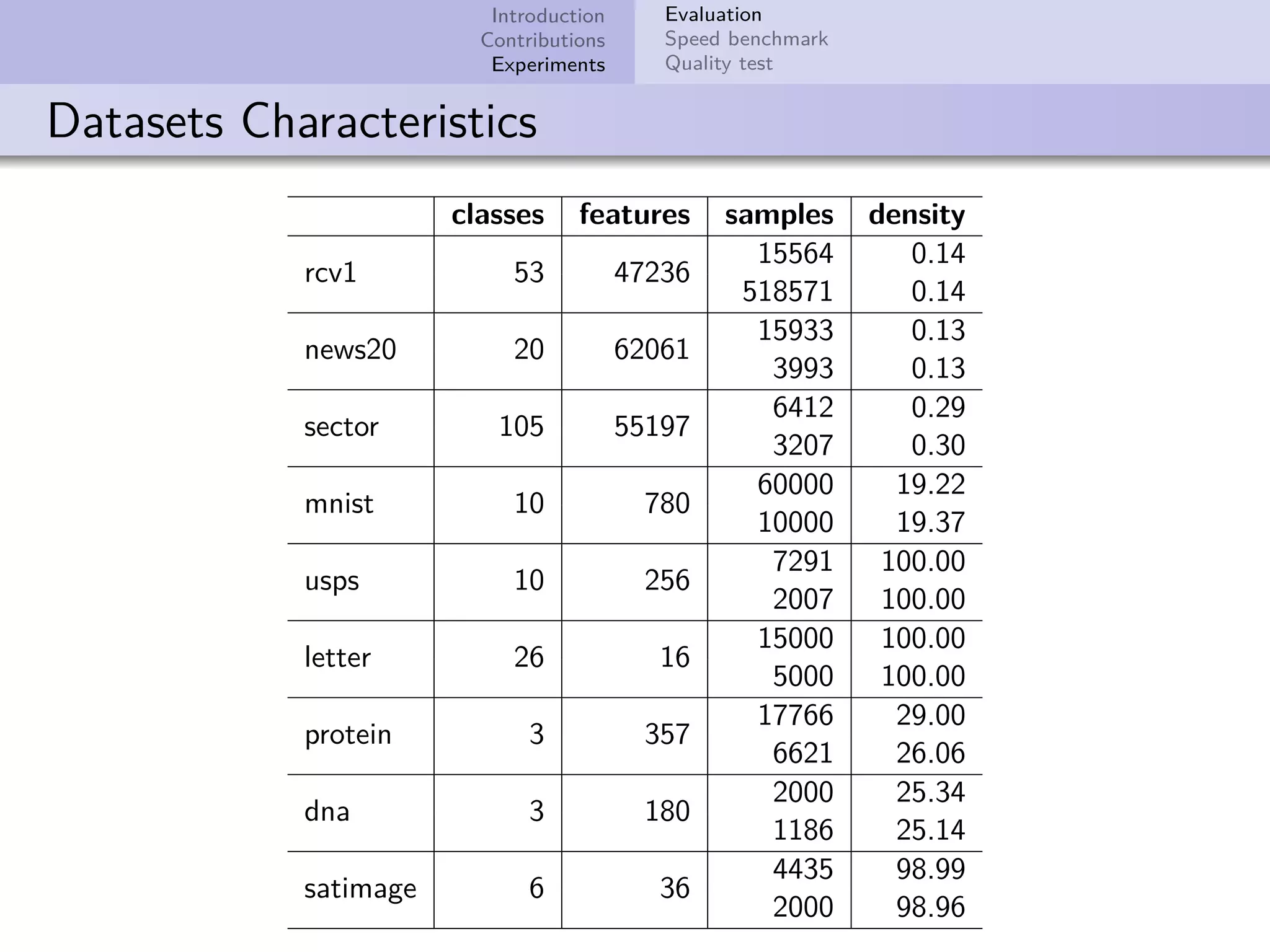
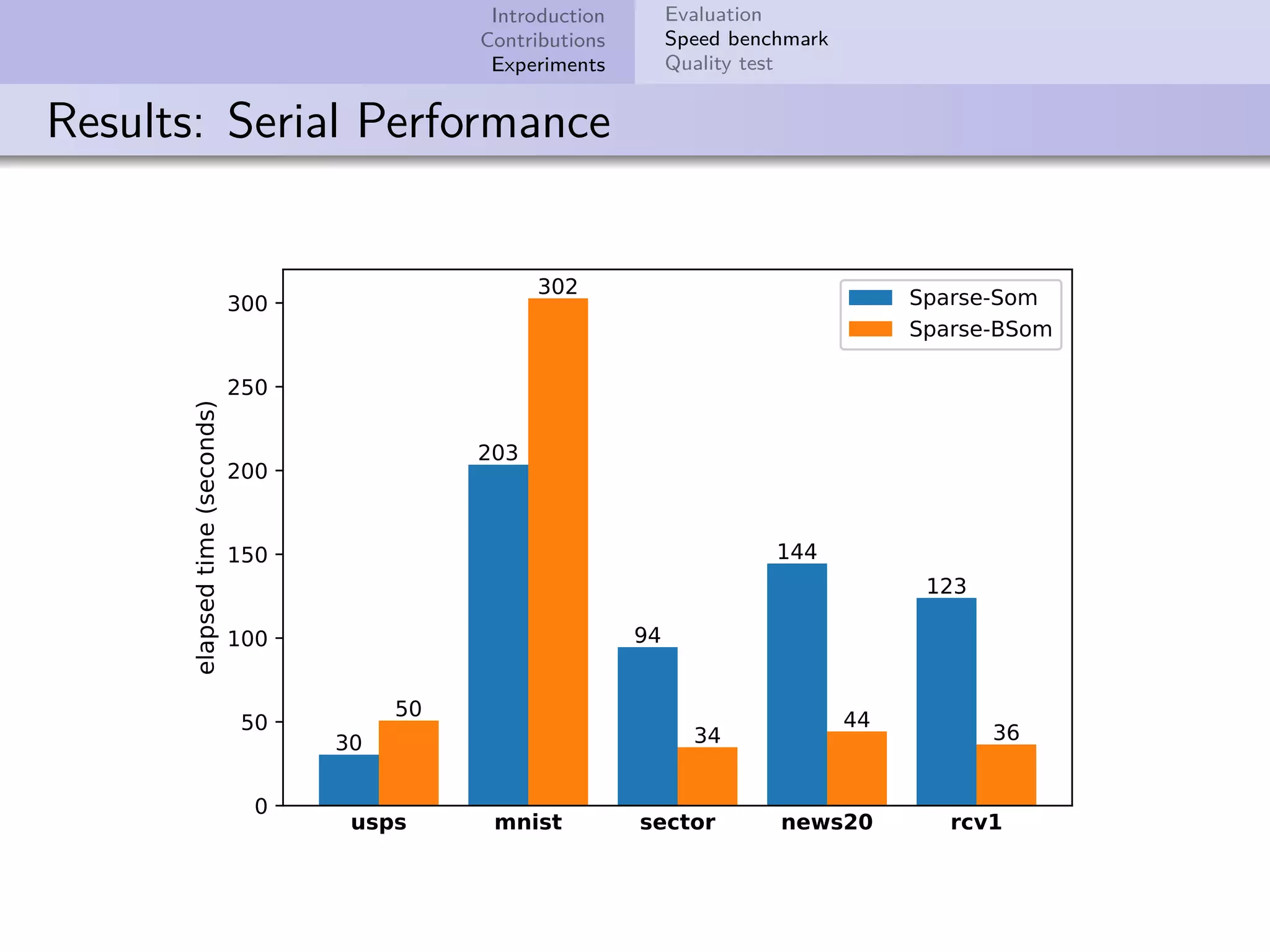
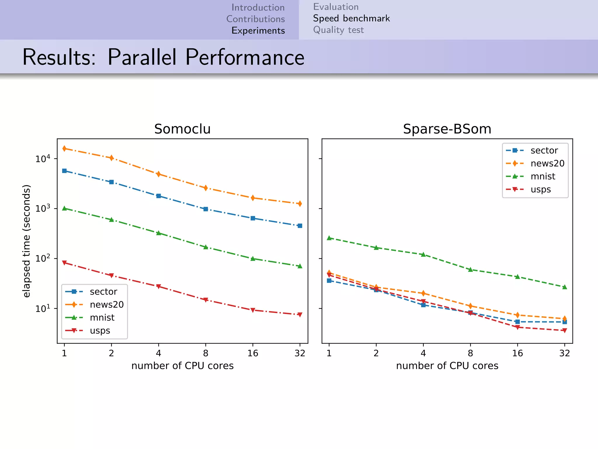
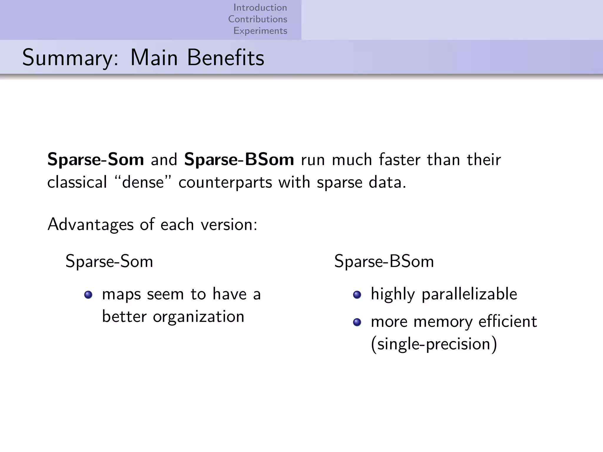
This document describes improvements made to the self-organizing map (SOM) algorithm to make it more efficient for sparse, high-dimensional input data. The key contributions are a sparse SOM (Sparse-Som) and sparse batch SOM (Sparse-BSom) algorithm that exploit the sparseness of the data to reduce computational complexity from O(TMD) to O(TMd), where d is the number of non-zero dimensions. Sparse-Som speeds up the BMU search and weight update phases, while Sparse-BSom further allows for efficient parallelization. Experiments show Sparse-Som and Sparse-BSom train significantly faster than standard SOM on sparse datasets, with comparable or better quality

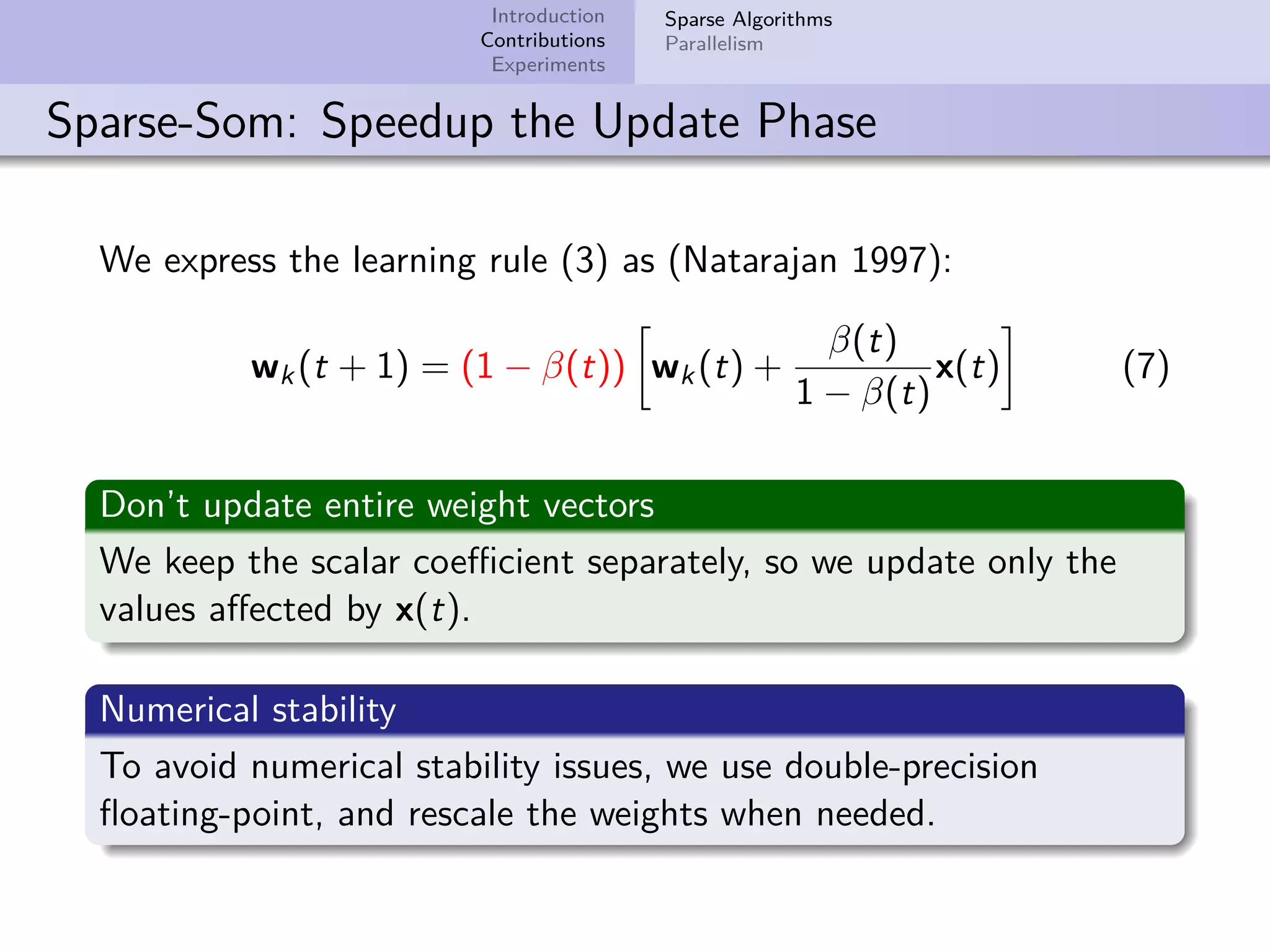
![Introduction Contributions Experiments SOM Description Standard vs. Batch Versions Motivation for Sparse SOM Standard Algorithm: The Learning Rule Update weight vectors at each time step, for a random sample x: wk(t + 1) = wk(t) + α(t)hck(t) [x(t) − wk(t)] (3) α(t) is the decreasing learning rate hck(t) is the neighborhood function For example, the Gaussian: hck(t) = exp − rk − rc 2 2σ(t)2 Gaussian neighborhood](https://image.slidesharecdn.com/presentation-171102132112/75/Efficient-Implementation-of-Self-Organizing-Map-for-Sparse-Input-Data-7-2048.jpg)