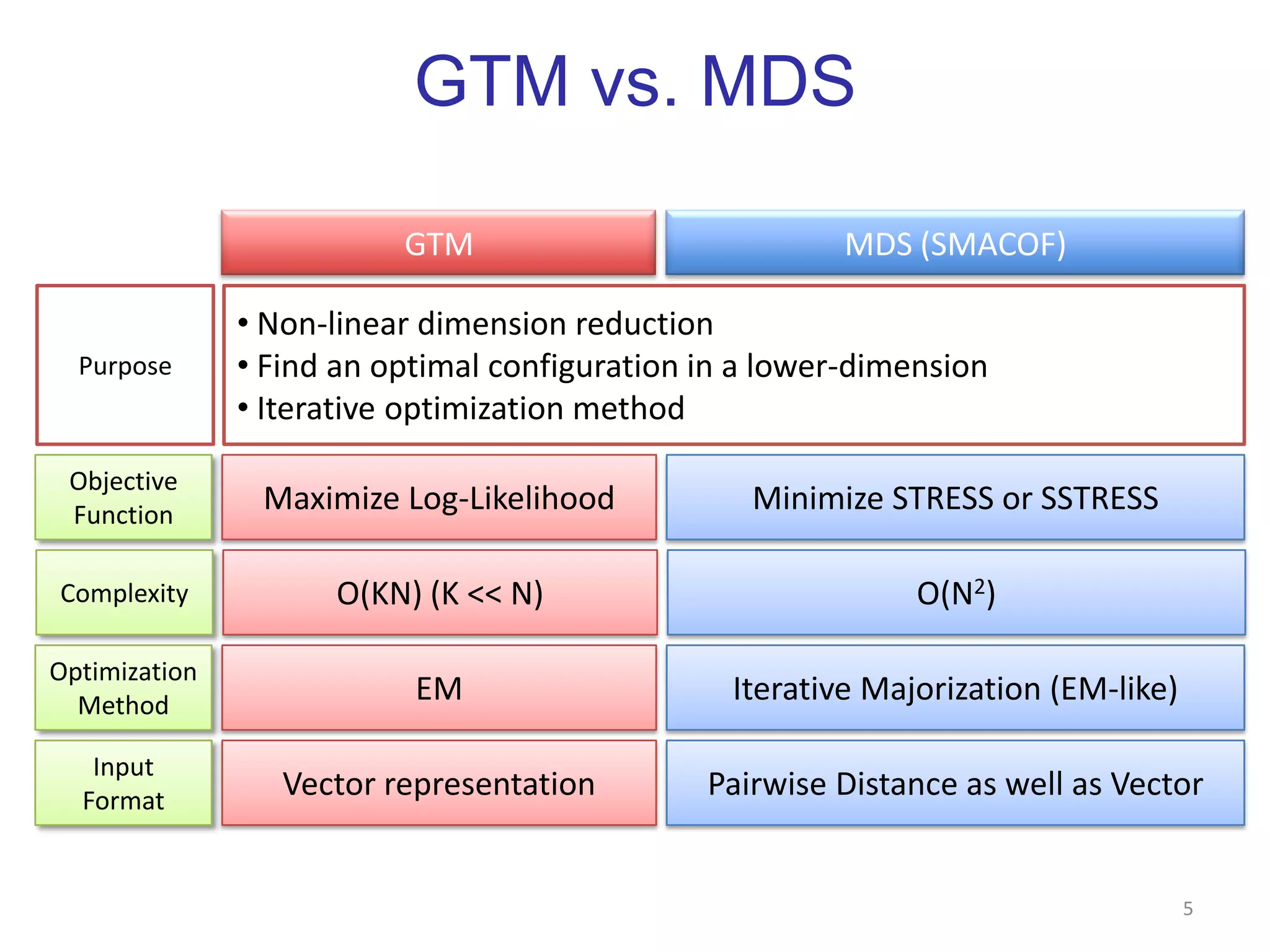
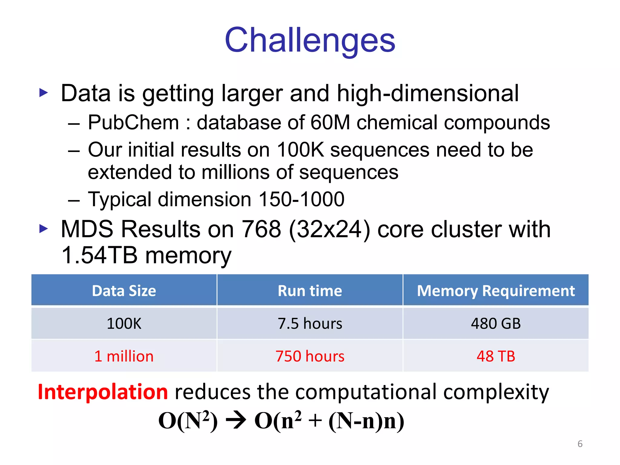
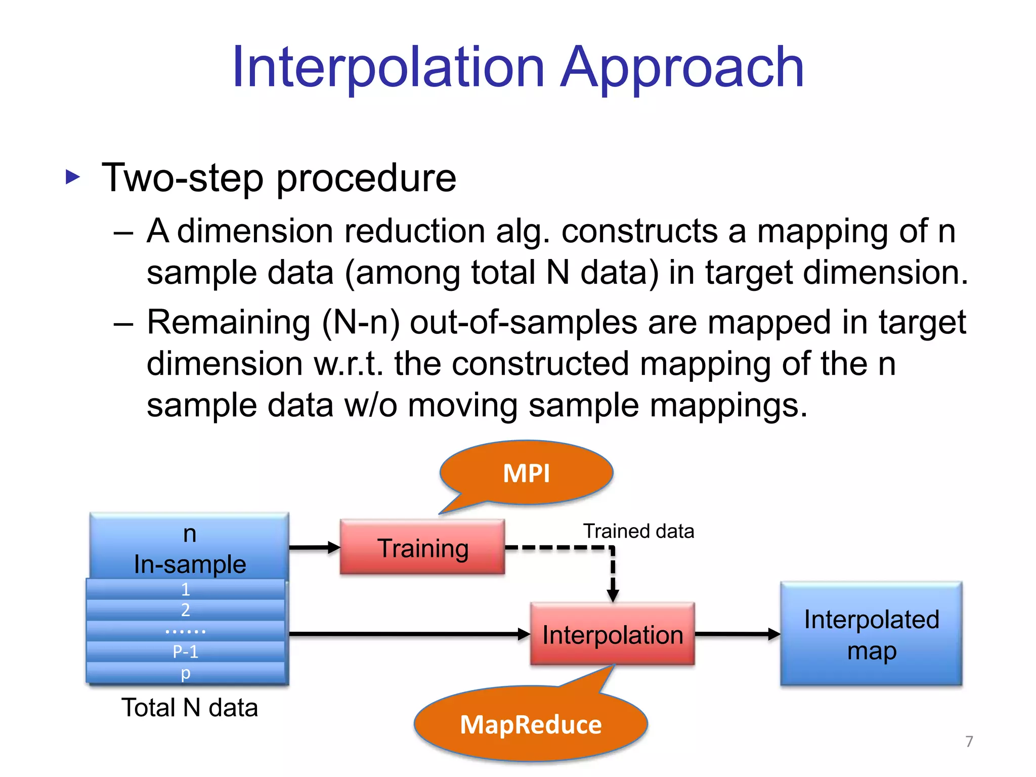
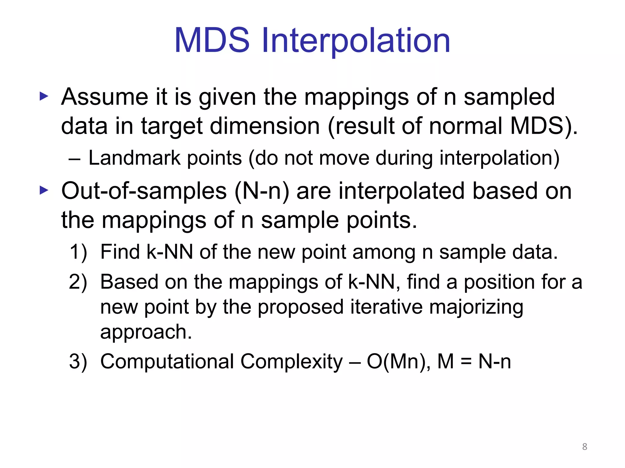
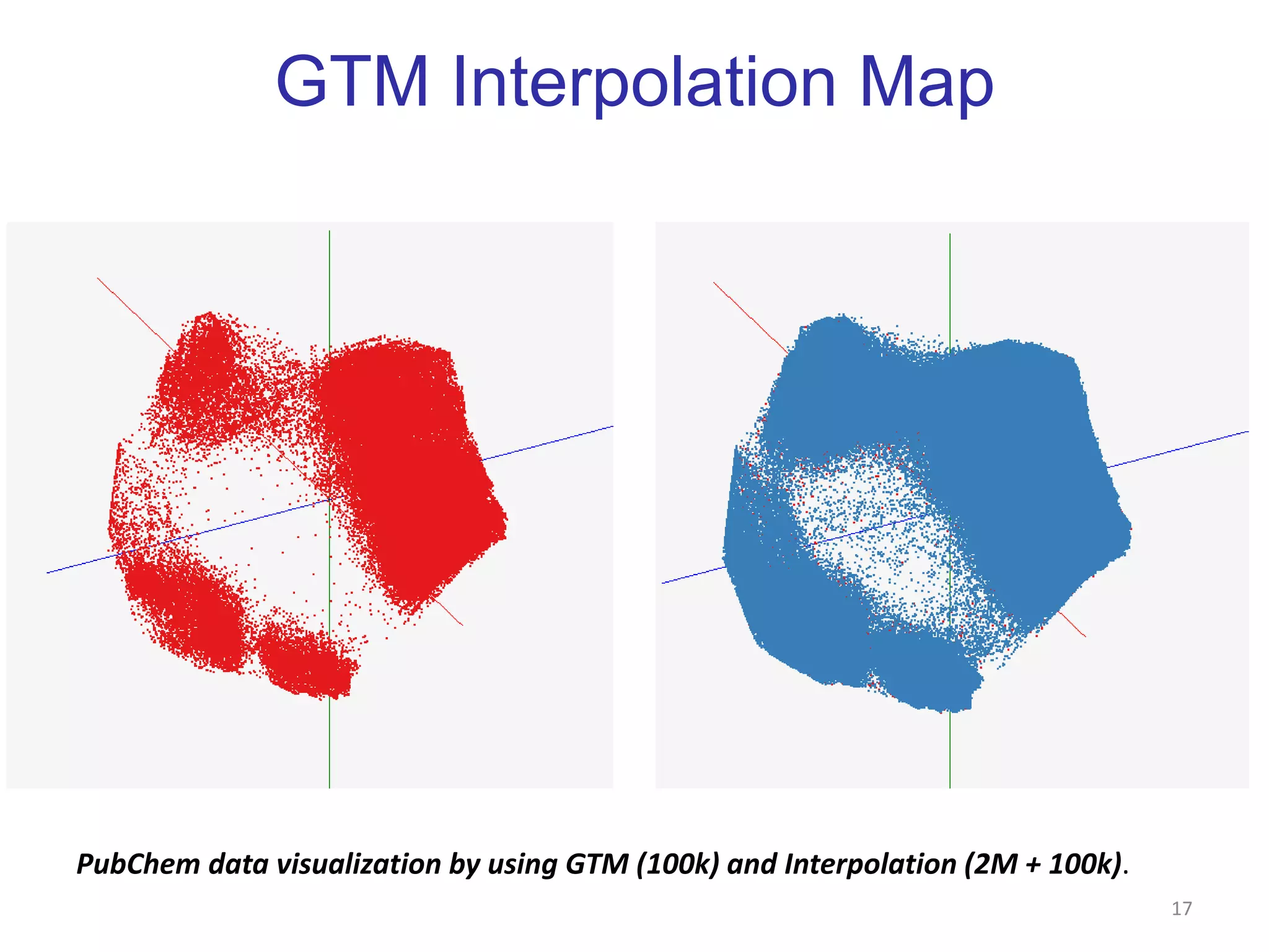
Dimension Reduction and Visualization of Large High-Dimensional Data via InterpolationSeung-HeeBae, Jong Youl Choi, Judy Qiu, and Geoffrey FoxSchool of Informatics and ComputingPervasive Technology InstituteIndiana UniversitySALSA projecthttp://salsahpc.indiana.edu
OutlineIntroduction to Point Data VisualizationReview of Dimension Reduction Algorithms.Multidimensional Scaling (MDS)Generative Topographic Mapping (GTM)ChallengesInterpolationMDS InterpolationGTM InterpolationExperimental ResultsConclusion1
Point Data VisualizationVisualize high-dimensional data as points in 2D or 3D by dimension reduction.Distances in target dimension approximate to the distances in the original HD space.Interactively browse dataEasy to recognize clusters or groupsAn example of chemical data (PubChem)Visualization to display disease-gene relationship, aiming at finding cause-effect relationships between disease and genes.2
Multi-Dimensional ScalingPairwise dissimilarity matrixN-by-N matrixEach element can be a distance, score, rank, … Given Δ, find a mapping in the target dimensionCriteria (or objective function)STRESSSSTRESSSMACOF is one of algorithms to solve MDS problem3
Generative Topographic MappingK latent pointsN data pointsInput is high-dimensional vector points Latent Variable Model (LVM)Define K latent variables (zk)Map K latent points to the data space by using a non-linear function f (by EM approach)Construct maps of data points in the latent space based on Gaussian Mixture Model 4
GTM vs. MDS5GTMMDS (SMACOF) Non-linear dimension reduction
 Find an optimal configuration in a lower-dimension
 Iterative optimization methodPurposeMaximize Log-LikelihoodMinimize STRESS or SSTRESSObjectiveFunctionO(KN) (K << N)O(N2)ComplexityEMIterative Majorization (EM-like)OptimizationMethodVector representationPairwise Distance as well as VectorInputFormat
ChallengesData is getting larger and high-dimensionalPubChem : database of 60M chemical compoundsOur initial results on 100K sequences need to be extended to millions of sequencesTypical dimension 150-1000MDS Results on 768 (32x24) core cluster with 1.54TB memory6Interpolation reduces the computational complexityO(N2)  O(n2 + (N-n)n)
Interpolation ApproachTwo-step procedureA dimension reduction alg. constructs a mapping of n sample data (among total N data) in target dimension.Remaining (N-n) out-of-samples are mapped in target dimension w.r.t. the constructed mapping of the n sample data w/o moving sample mappings.MPInIn-sampleTrained dataTrainingN-nOut-of-sampleInterpolated map71Interpolation2......P-1pTotal N dataMapReduce
MDS InterpolationAssume it is given the mappings of n sampled data in target dimension (result of normal MDS).Landmark points (do not move during interpolation)Out-of-samples (N-n) are interpolated based on the mappings of n sample points.Find k-NN of the new point among n sample data.Based on the mappings of k-NN, find a position for a new point by the proposed iterative majorizing approach.Computational Complexity – O(Mn), M = N-n8
GTM InterpolationAssume it is given the position of K latent points based on the sample data in the latent space.The most time consuming part of GTMOut-of-samples (N-n) are positioned directly w.r.t. Gaussian Mixture Model between the new point and the given position of K latent points.Computational Complexity – O(M), M = N-n9
Experiment Environments10
Quality Comparison (1)11GTM interpolation quality comparisonw.r.t. different sample size of N = 100kMDS interpolation quality comparisonw.r.t. different sample size of N = 100k
Quality Comparison (2)12GTM interpolation quality up to 2MMDS interpolation quality up to 2M
Parallel Efficiency13MDS parallel efficiency on Cluster-IIGTM parallel efficiency on Cluster-II
GTM Interpolation via MapReduce14GTM Interpolation–Time per core to process 100k data points per coreGTM Interpolationparallel efficiency26.4 million pubchem data
DryadLINQ using a 16 core machine with 16 GB, Hadoop 8 core with 48 GB, Azure small instances with 1 core with 1.7 GB.ThilinaGunarathne, Tak-Lon Wu, Judy Qiu, and Geoffrey Fox, “Cloud Computing Paradigms for Pleasingly Parallel Biomedical Applications,” in Proceedings of ECMLS Workshop of ACM HPDC 2010
MDS Interpolation via MapReduce15DryadLINQ on 32 nodes X 24 Cores cluster with 48 GB per node. Azure using small instancesThilinaGunarathne, Tak-Lon Wu, Judy Qiu, and Geoffrey Fox, “Cloud Computing Paradigms for Pleasingly Parallel Biomedical Applications,” in Proceedings of ECMLS Workshop of ACM HPDC 2010
MDS Interpolation Map16PubChem data visualization by using MDS (100k) and Interpolation (100k+100k).
GTM Interpolation Map17PubChem data visualization by using GTM (100k) and Interpolation (2M + 100k).
ConclusionDimension reduction algorithms (e.g. GTM and MDS) are computation and memory intensive applications.Apply interpolation (out-of-sample) approach to GTM and MDS in order to process and visualize large- and high-dimensional dataset.It is possible to process millions data point via interpolation.Could be parallelized by MapReduce fashion as well as MPI fashion.18
Future WorksMake available as a ServiceHierarchical Interpolation could reduce the computational complexity	O(Mn) O(Mlog(n))19
AcknowledgmentOur internal collaborators in School of Informatics and Computing at IUBProf. David WildDr. Qian Zhu20

Dimension Reduction And Visualization Of Large High Dimensional Data Via Interpolation

  • 1.
    Dimension Reduction andVisualization of Large High-Dimensional Data via InterpolationSeung-HeeBae, Jong Youl Choi, Judy Qiu, and Geoffrey FoxSchool of Informatics and ComputingPervasive Technology InstituteIndiana UniversitySALSA projecthttp://salsahpc.indiana.edu
  • 2.
    OutlineIntroduction to PointData VisualizationReview of Dimension Reduction Algorithms.Multidimensional Scaling (MDS)Generative Topographic Mapping (GTM)ChallengesInterpolationMDS InterpolationGTM InterpolationExperimental ResultsConclusion1
  • 3.
    Point Data VisualizationVisualizehigh-dimensional data as points in 2D or 3D by dimension reduction.Distances in target dimension approximate to the distances in the original HD space.Interactively browse dataEasy to recognize clusters or groupsAn example of chemical data (PubChem)Visualization to display disease-gene relationship, aiming at finding cause-effect relationships between disease and genes.2
  • 4.
    Multi-Dimensional ScalingPairwise dissimilaritymatrixN-by-N matrixEach element can be a distance, score, rank, … Given Δ, find a mapping in the target dimensionCriteria (or objective function)STRESSSSTRESSSMACOF is one of algorithms to solve MDS problem3
  • 5.
    Generative Topographic MappingKlatent pointsN data pointsInput is high-dimensional vector points Latent Variable Model (LVM)Define K latent variables (zk)Map K latent points to the data space by using a non-linear function f (by EM approach)Construct maps of data points in the latent space based on Gaussian Mixture Model 4
  • 6.
    GTM vs. MDS5GTMMDS(SMACOF) Non-linear dimension reduction
  • 7.
    Find anoptimal configuration in a lower-dimension
  • 8.
    Iterative optimizationmethodPurposeMaximize Log-LikelihoodMinimize STRESS or SSTRESSObjectiveFunctionO(KN) (K << N)O(N2)ComplexityEMIterative Majorization (EM-like)OptimizationMethodVector representationPairwise Distance as well as VectorInputFormat
  • 9.
    ChallengesData is gettinglarger and high-dimensionalPubChem : database of 60M chemical compoundsOur initial results on 100K sequences need to be extended to millions of sequencesTypical dimension 150-1000MDS Results on 768 (32x24) core cluster with 1.54TB memory6Interpolation reduces the computational complexityO(N2)  O(n2 + (N-n)n)
  • 10.
    Interpolation ApproachTwo-step procedureAdimension reduction alg. constructs a mapping of n sample data (among total N data) in target dimension.Remaining (N-n) out-of-samples are mapped in target dimension w.r.t. the constructed mapping of the n sample data w/o moving sample mappings.MPInIn-sampleTrained dataTrainingN-nOut-of-sampleInterpolated map71Interpolation2......P-1pTotal N dataMapReduce
  • 11.
    MDS InterpolationAssume itis given the mappings of n sampled data in target dimension (result of normal MDS).Landmark points (do not move during interpolation)Out-of-samples (N-n) are interpolated based on the mappings of n sample points.Find k-NN of the new point among n sample data.Based on the mappings of k-NN, find a position for a new point by the proposed iterative majorizing approach.Computational Complexity – O(Mn), M = N-n8
  • 12.
    GTM InterpolationAssume itis given the position of K latent points based on the sample data in the latent space.The most time consuming part of GTMOut-of-samples (N-n) are positioned directly w.r.t. Gaussian Mixture Model between the new point and the given position of K latent points.Computational Complexity – O(M), M = N-n9
  • 13.
  • 14.
    Quality Comparison (1)11GTMinterpolation quality comparisonw.r.t. different sample size of N = 100kMDS interpolation quality comparisonw.r.t. different sample size of N = 100k
  • 15.
    Quality Comparison (2)12GTMinterpolation quality up to 2MMDS interpolation quality up to 2M
  • 16.
    Parallel Efficiency13MDS parallelefficiency on Cluster-IIGTM parallel efficiency on Cluster-II
  • 17.
    GTM Interpolation viaMapReduce14GTM Interpolation–Time per core to process 100k data points per coreGTM Interpolationparallel efficiency26.4 million pubchem data
  • 18.
    DryadLINQ using a16 core machine with 16 GB, Hadoop 8 core with 48 GB, Azure small instances with 1 core with 1.7 GB.ThilinaGunarathne, Tak-Lon Wu, Judy Qiu, and Geoffrey Fox, “Cloud Computing Paradigms for Pleasingly Parallel Biomedical Applications,” in Proceedings of ECMLS Workshop of ACM HPDC 2010
  • 19.
    MDS Interpolation viaMapReduce15DryadLINQ on 32 nodes X 24 Cores cluster with 48 GB per node. Azure using small instancesThilinaGunarathne, Tak-Lon Wu, Judy Qiu, and Geoffrey Fox, “Cloud Computing Paradigms for Pleasingly Parallel Biomedical Applications,” in Proceedings of ECMLS Workshop of ACM HPDC 2010
  • 20.
    MDS Interpolation Map16PubChemdata visualization by using MDS (100k) and Interpolation (100k+100k).
  • 21.
    GTM Interpolation Map17PubChemdata visualization by using GTM (100k) and Interpolation (2M + 100k).
  • 22.
    ConclusionDimension reduction algorithms(e.g. GTM and MDS) are computation and memory intensive applications.Apply interpolation (out-of-sample) approach to GTM and MDS in order to process and visualize large- and high-dimensional dataset.It is possible to process millions data point via interpolation.Could be parallelized by MapReduce fashion as well as MPI fashion.18
  • 23.
    Future WorksMake availableas a ServiceHierarchical Interpolation could reduce the computational complexity O(Mn) O(Mlog(n))19
  • 24.
    AcknowledgmentOur internal collaboratorsin School of Informatics and Computing at IUBProf. David WildDr. Qian Zhu20
  • 25.
    Thank youQuestion?Email meat sebae@cs.indiana.edu21
  • 26.
    EM optimizationFind Kcenters for N data K-clustering problem, known as NP-hardUse Expectation-Maximization (EM) methodEM algorithmFind local optimal solution iteratively until convergeE-step:M-step:22
  • 27.
    ParallelizationInterpolation is pleasinglyparallel applicationOut-of-sample data are independent each other.We can parallelize interpolation app. by MapReduce fashion as well as MPI fashion.ThilinaGunarathne, Tak-Lon Wu, Judy Qiu, and Geoffrey Fox, “Cloud Computing Paradigms for Pleasingly Parallel Biomedical Applications,” in Proceedings of ECMLS Workshop of ACM HPDC 201023nIn-sampleTrained dataTrainingN-nOut-of-sampleInterpolated map1Interpolation2......P-1pTotal N data

Editor's Notes

  • #4 Microarray data
  • #15 EC2 HM4XL - High memory large instances (8 * 3.25 Ghz cores, 68GB memory)EC2 HCXL – High CPU extra large (8 * 2.4 Ghz, 7GB memory)EC2 Large – 2 * 2.4 Ghz , 7.5 GB memoryGTM interpolation is memory bound. Hence, less cores per memory (less memory &amp; memory bandwidth contention) has the advantage. DryadLINQ efficiency suffers due to 16 core 16 GB machines.
  • #16 Efficiency drop in MDS DryadLINQ at the last point is due to unbalanced partition (2600 blocks in to 768 cores)