Download as PDF, PPTX
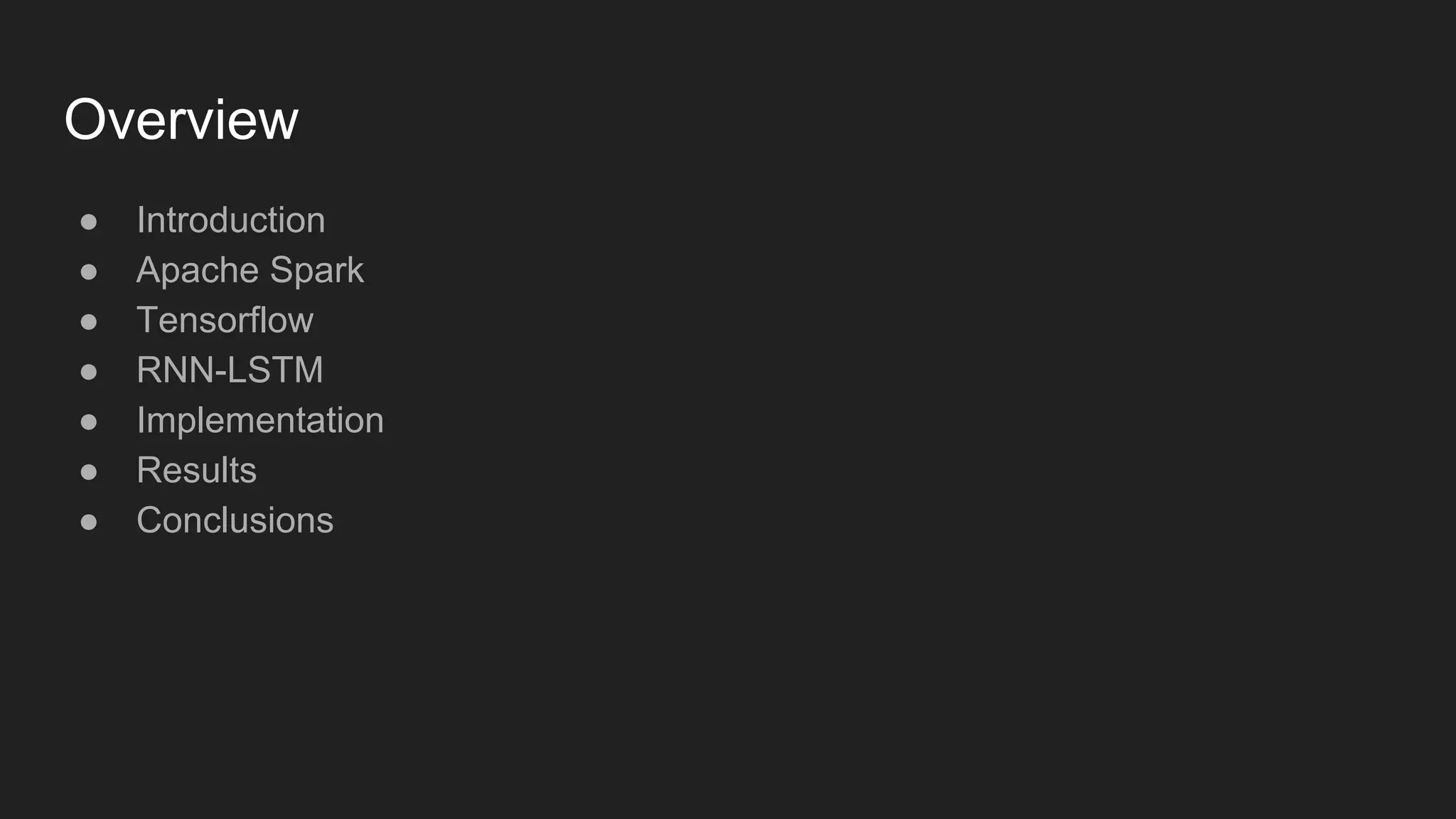
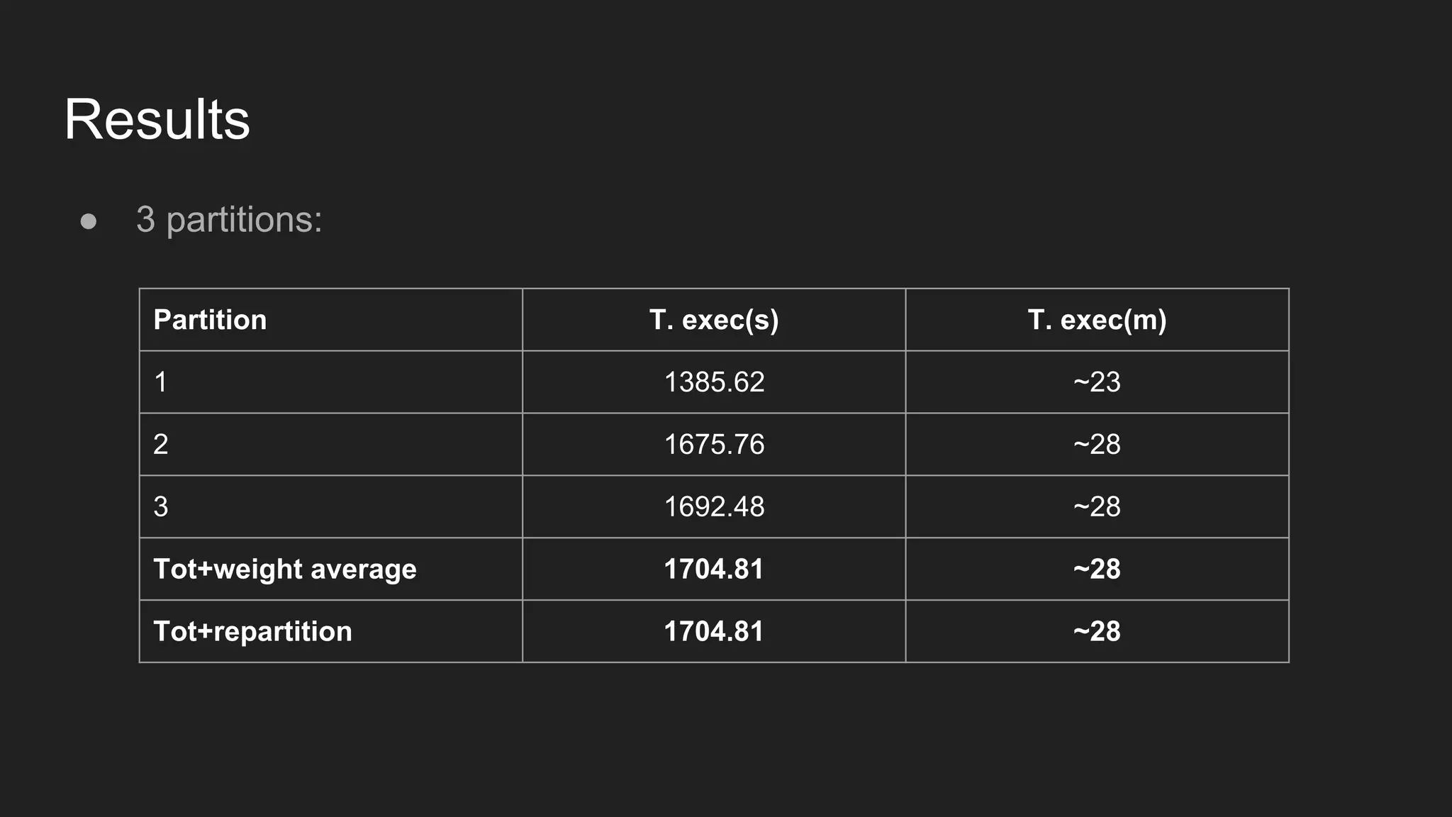
![Results ● 3 partitions [overloaded vs idle]: Part. T. exec busy(s) T. exec busy(m) T. exec idle(s) T. exec idle(m) 1 2679.76 ~44 1385.62 ~23 2 2910.69 ~48 1675.76 ~28 3 3063.88 ~51 1692.48 ~28 Tot 3078.15 ~51 1704.81 ~28](https://image.slidesharecdn.com/distributedimplementationofalstmonsparkandtensorflow-161203125800/75/Distributed-implementation-of-a-lstm-on-spark-and-tensorflow-23-2048.jpg)
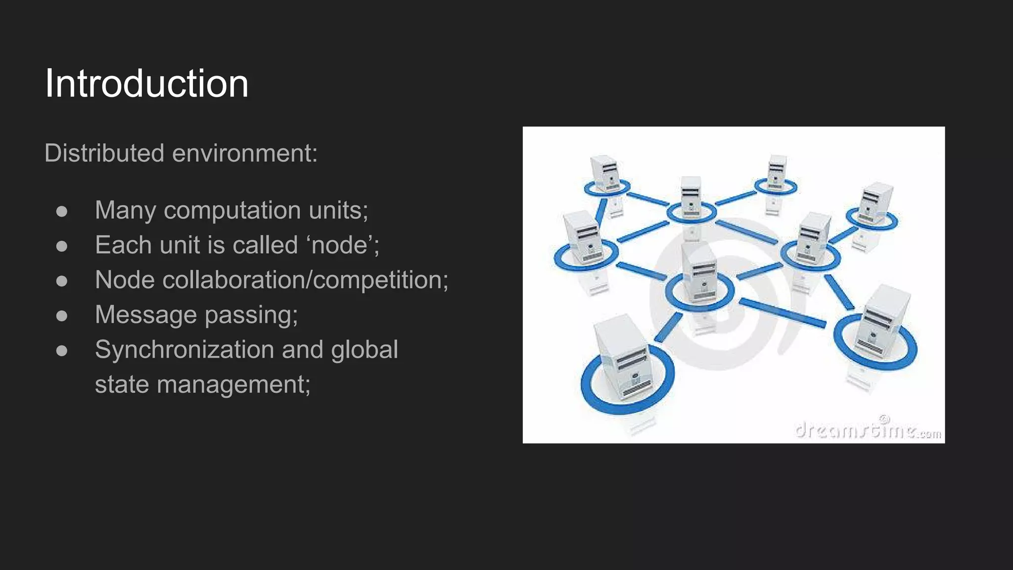
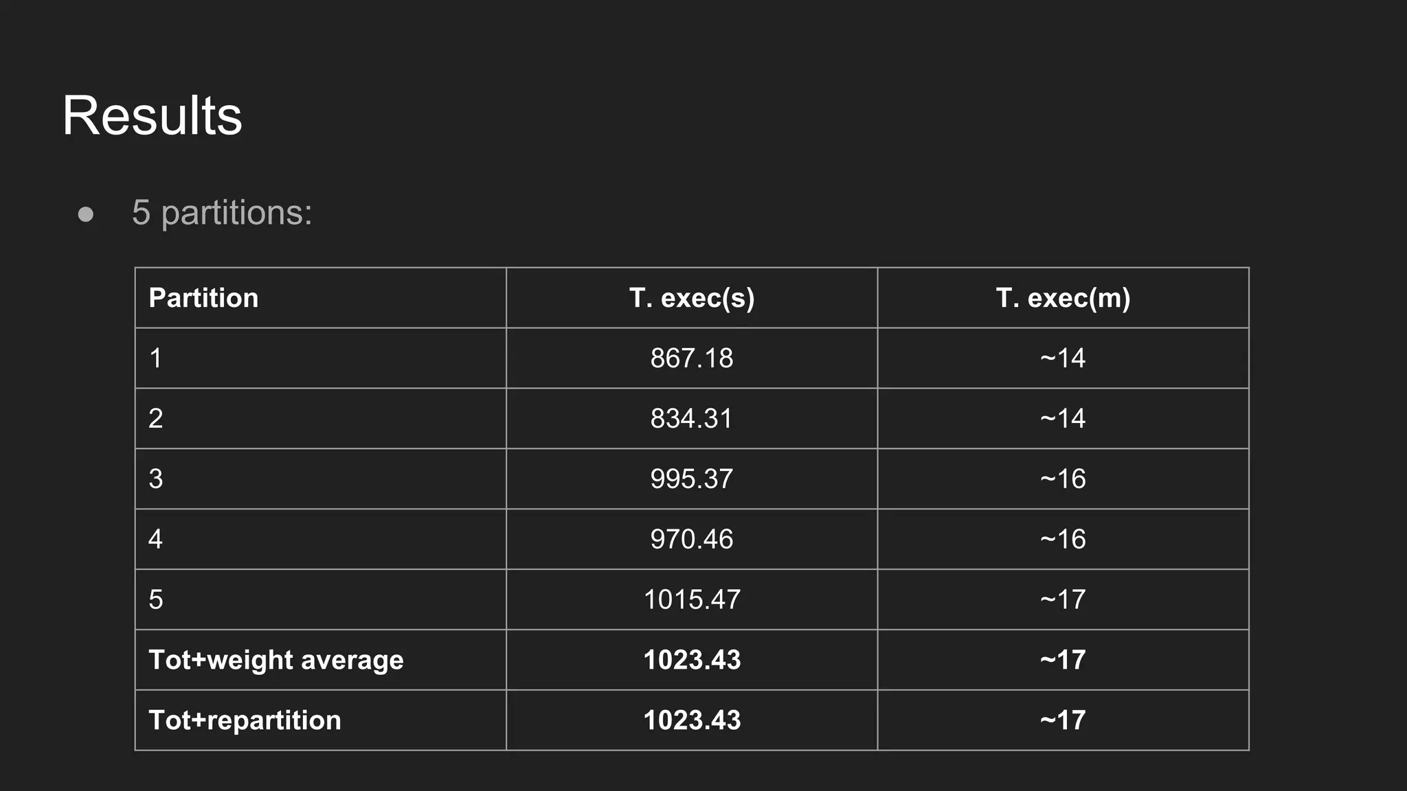
![Results ● 5 partitions [overloaded vs idle]: Part. T. exec busy(s) T. exec busy(m) T. exec idle(s) T. exec idle(m) 1 1356.44 ~22 867.18 ~14 2 1358.28 ~22 834.31 ~14 3 1373.25 ~22 995.37 ~16 4 1370.11 ~23 970.46 ~16 5 1372.25 ~23 1015.47 ~17 Tot 1393.91 ~23 1023.43 ~17](https://image.slidesharecdn.com/distributedimplementationofalstmonsparkandtensorflow-161203125800/75/Distributed-implementation-of-a-lstm-on-spark-and-tensorflow-24-2048.jpg)

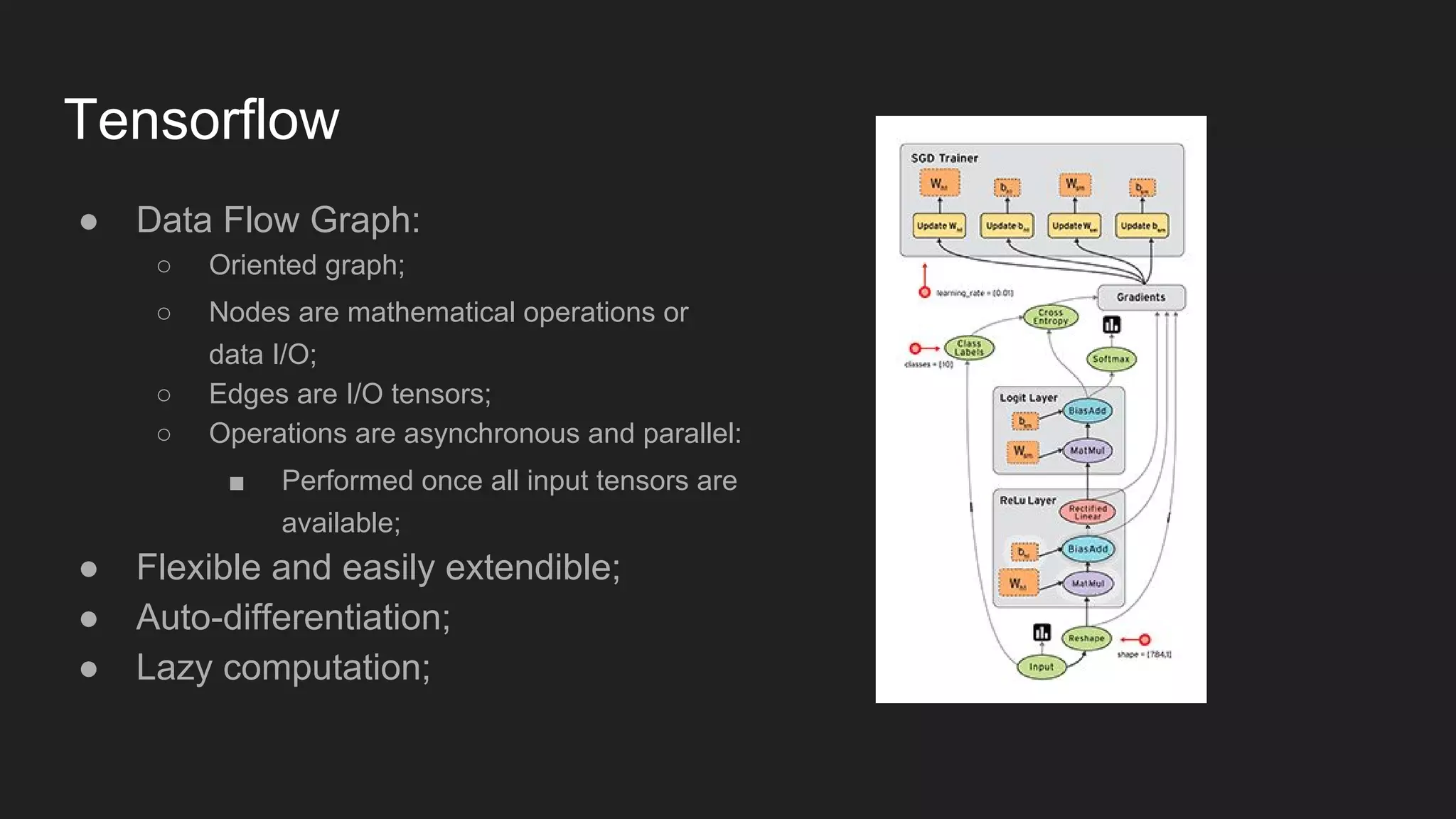
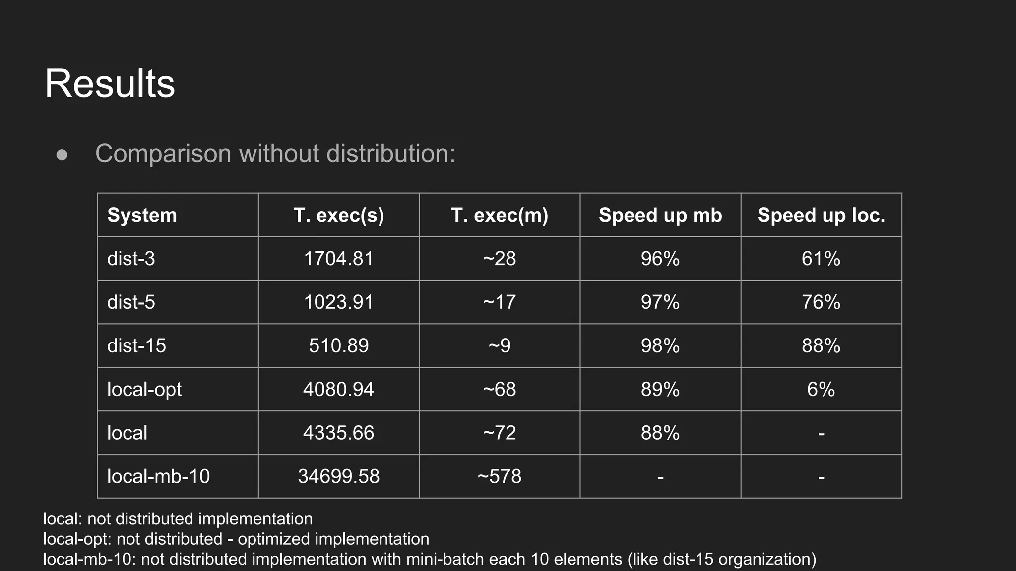
The document discusses the distributed implementation of LSTM models using Apache Spark and TensorFlow, focusing on the architecture and functionalities of each framework. It details the process of distributing training tasks across nodes, including data partitioning and mini-batch strategies, and presents performance results from various configurations. The findings highlight improved training times with distributed processing compared to local execution.