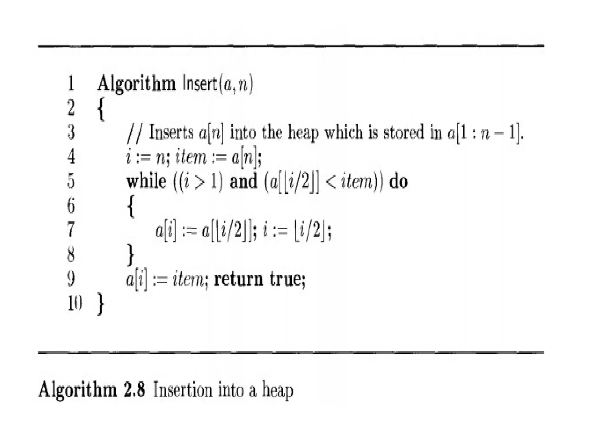
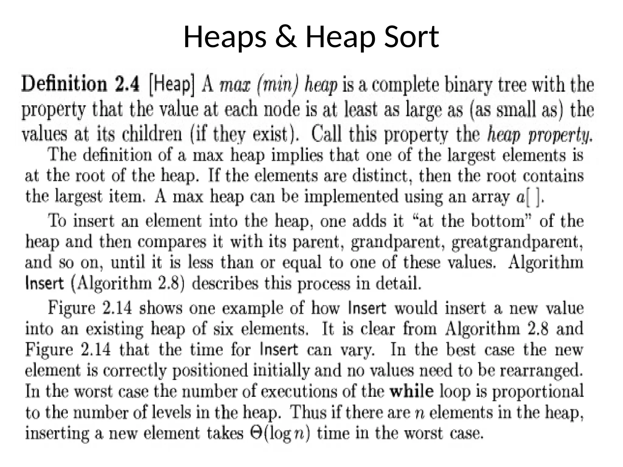
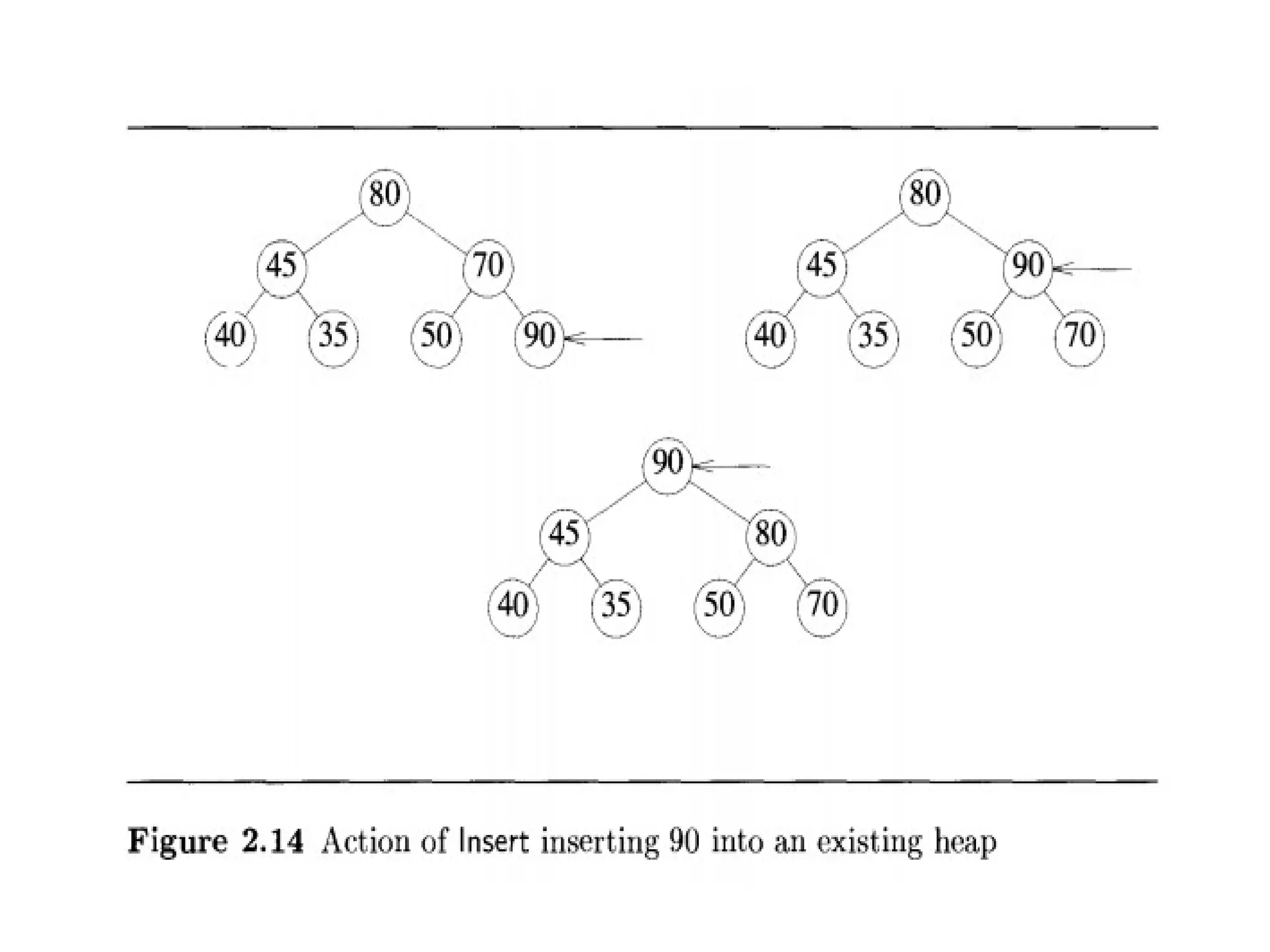
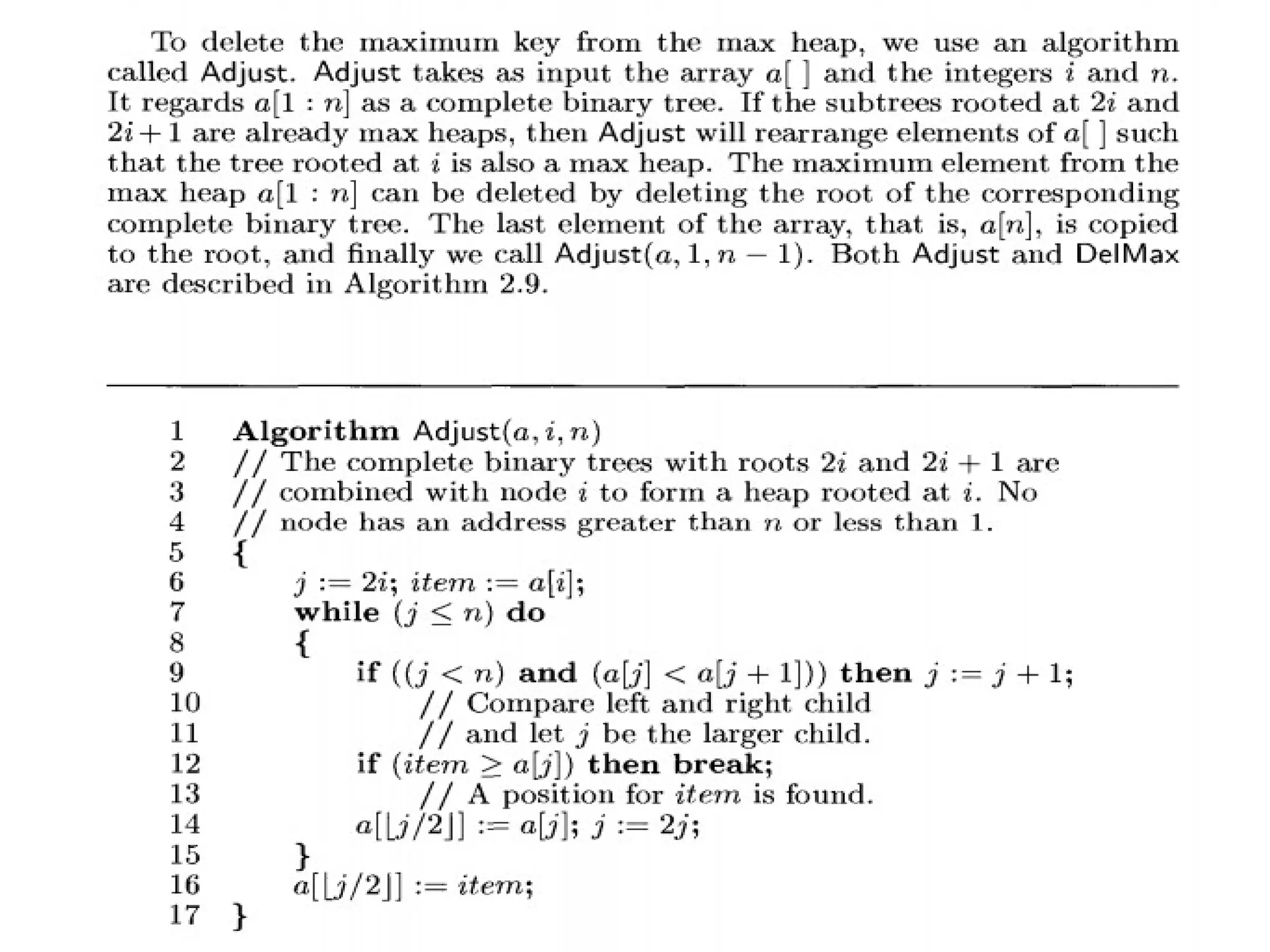
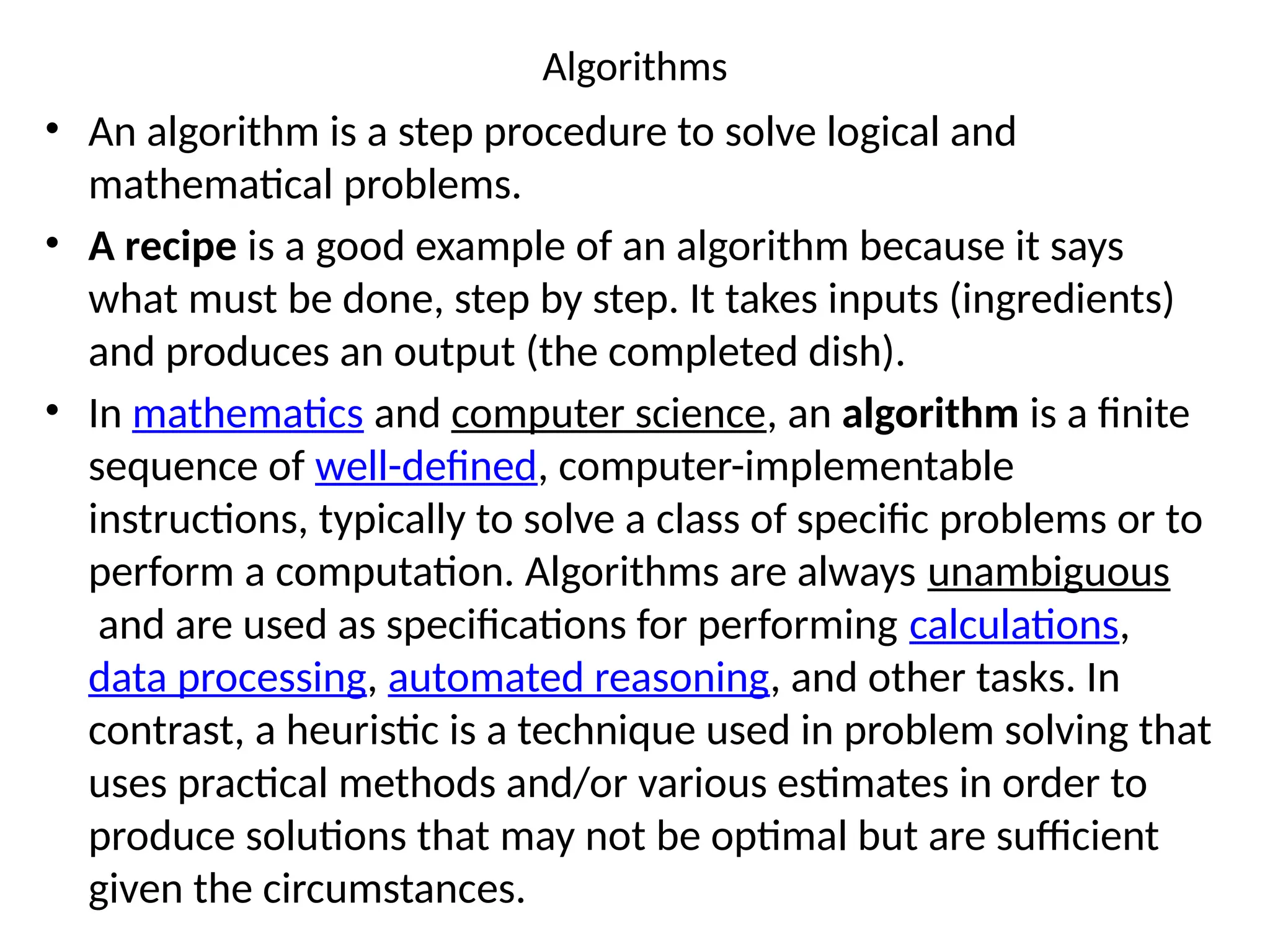
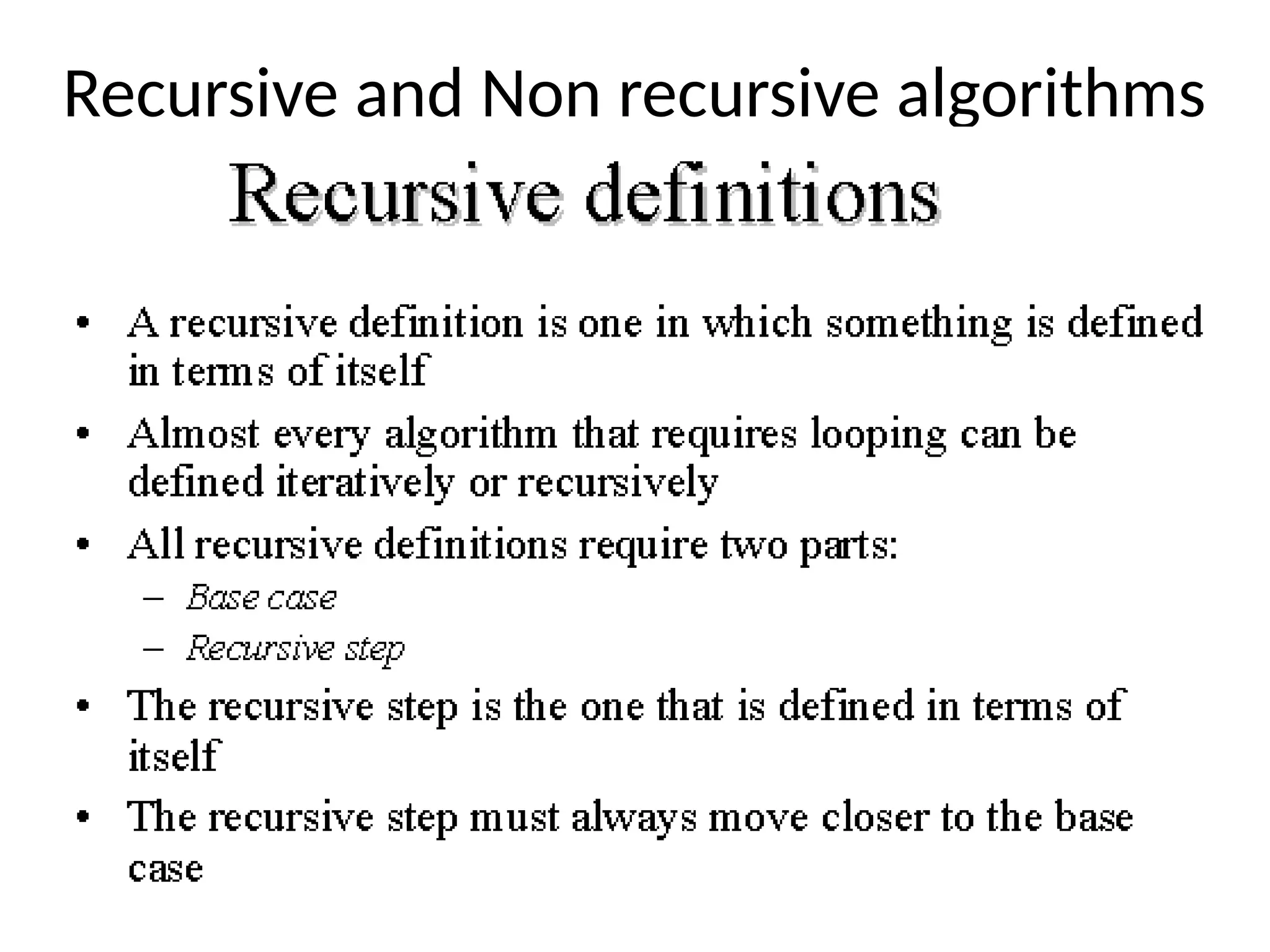
Algorithms • An algorithmis a step procedure to solve logical and mathematical problems. • A recipe is a good example of an algorithm because it says what must be done, step by step. It takes inputs (ingredients) and produces an output (the completed dish). • In mathematics and computer science, an algorithm is a finite sequence of well-defined, computer-implementable instructions, typically to solve a class of specific problems or to perform a computation. Algorithms are always unambiguous and are used as specifications for performing calculations, data processing, automated reasoning, and other tasks. In contrast, a heuristic is a technique used in problem solving that uses practical methods and/or various estimates in order to produce solutions that may not be optimal but are sufficient given the circumstances.
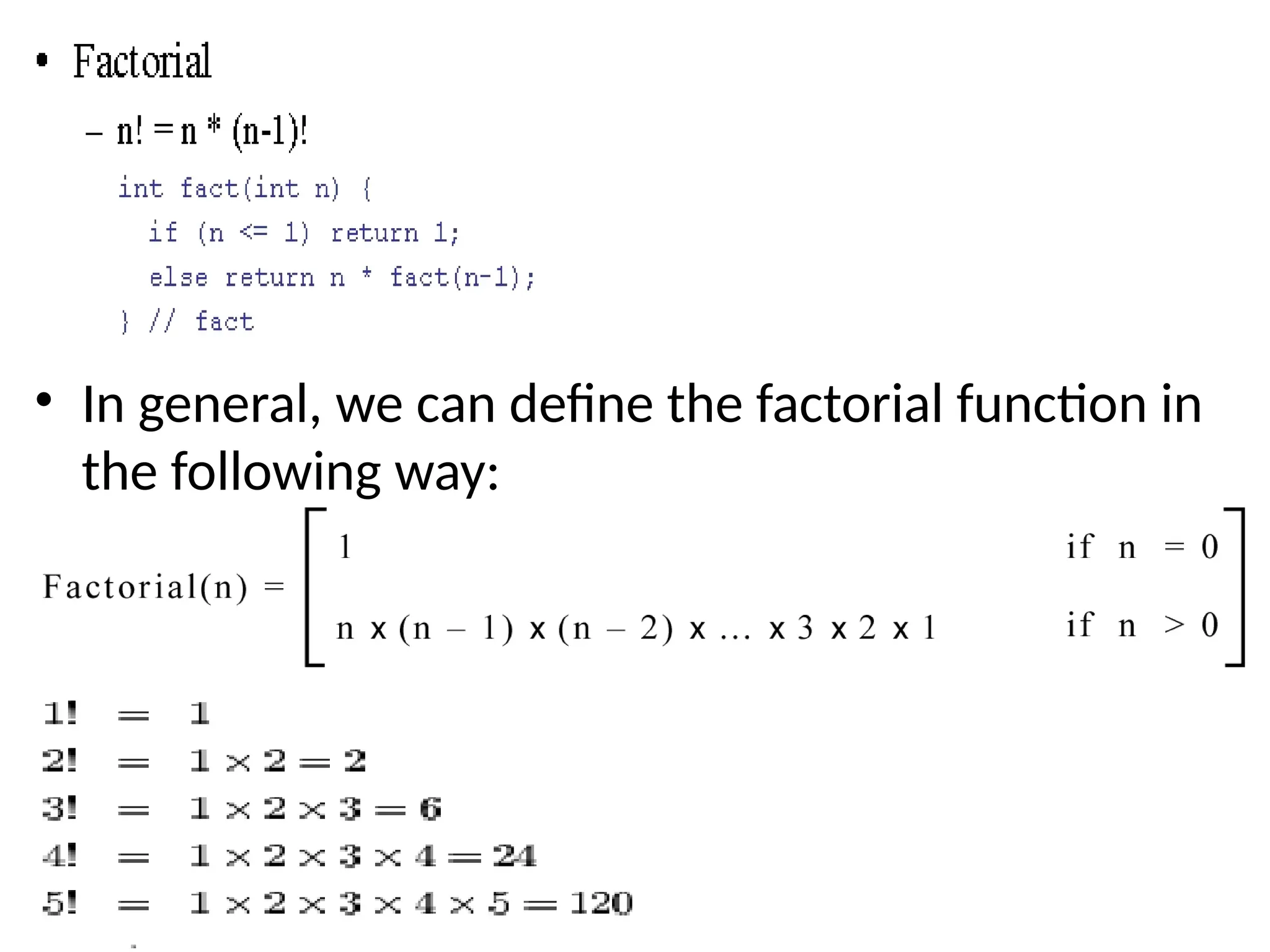
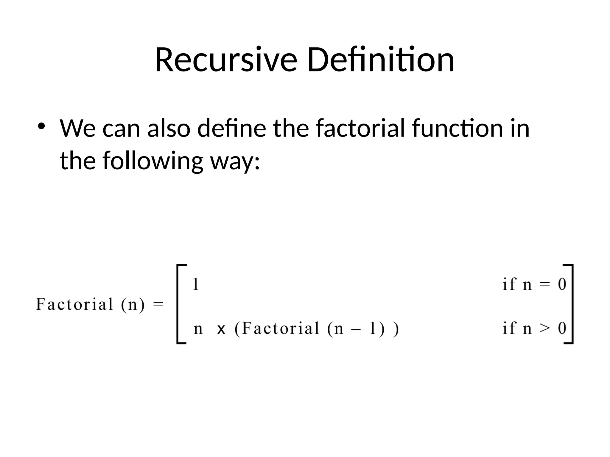
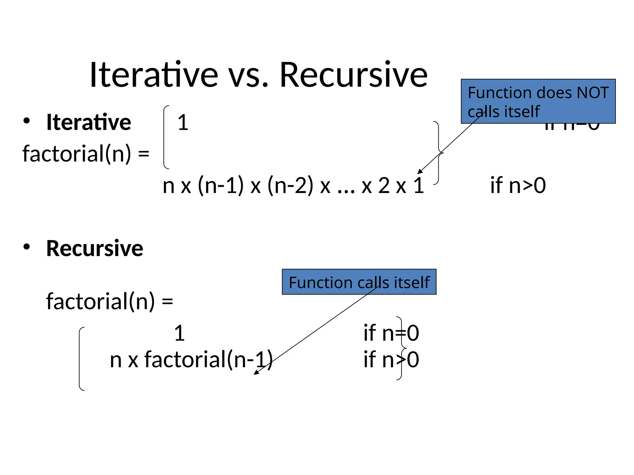
• In general,we can define the factorial function in the following way:
6.
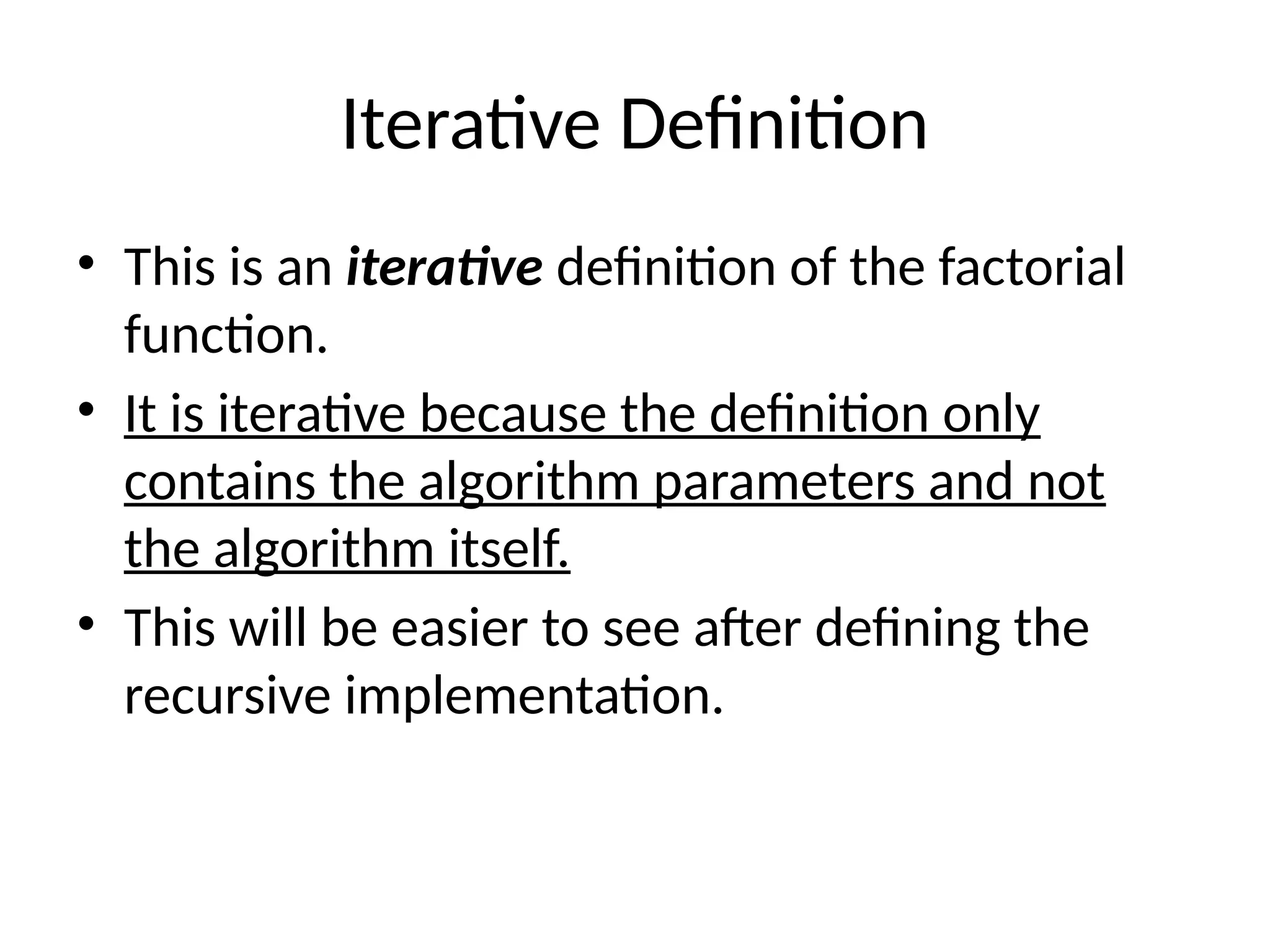
Iterative Definition • Thisis an iterative definition of the factorial function. • It is iterative because the definition only contains the algorithm parameters and not the algorithm itself. • This will be easier to see after defining the recursive implementation.
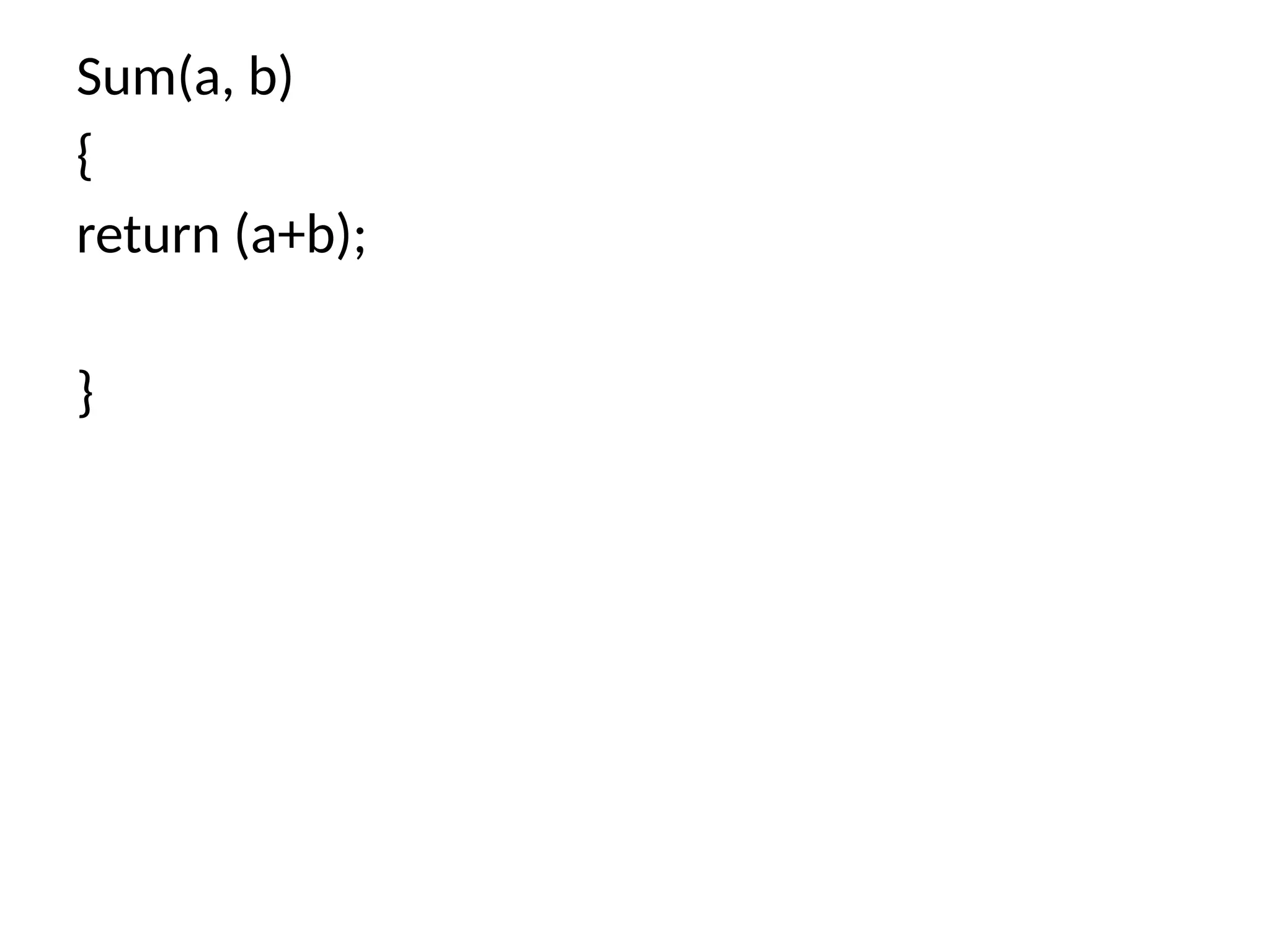
Iterative vs. Recursive •Iterative 1 if n=0 factorial(n) = n x (n-1) x (n-2) x … x 2 x 1 if n>0 • Recursive factorial(n) = 1 if n=0 n x factorial(n-1) if n>0 Function calls itself Function does NOT calls itself
10.
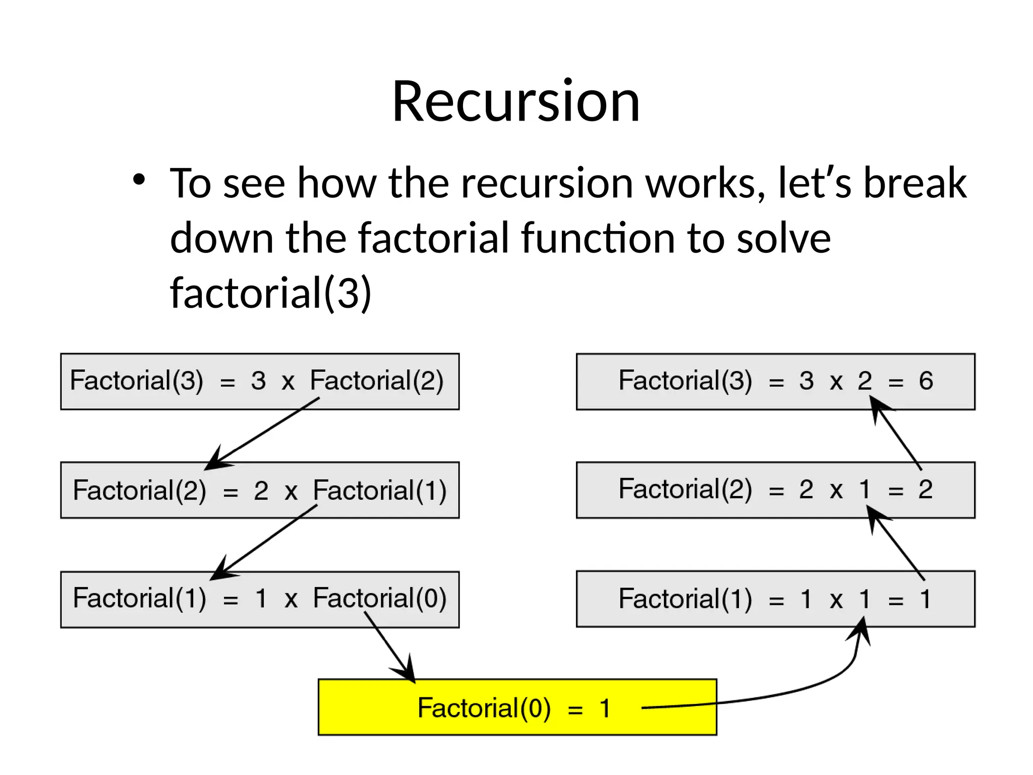
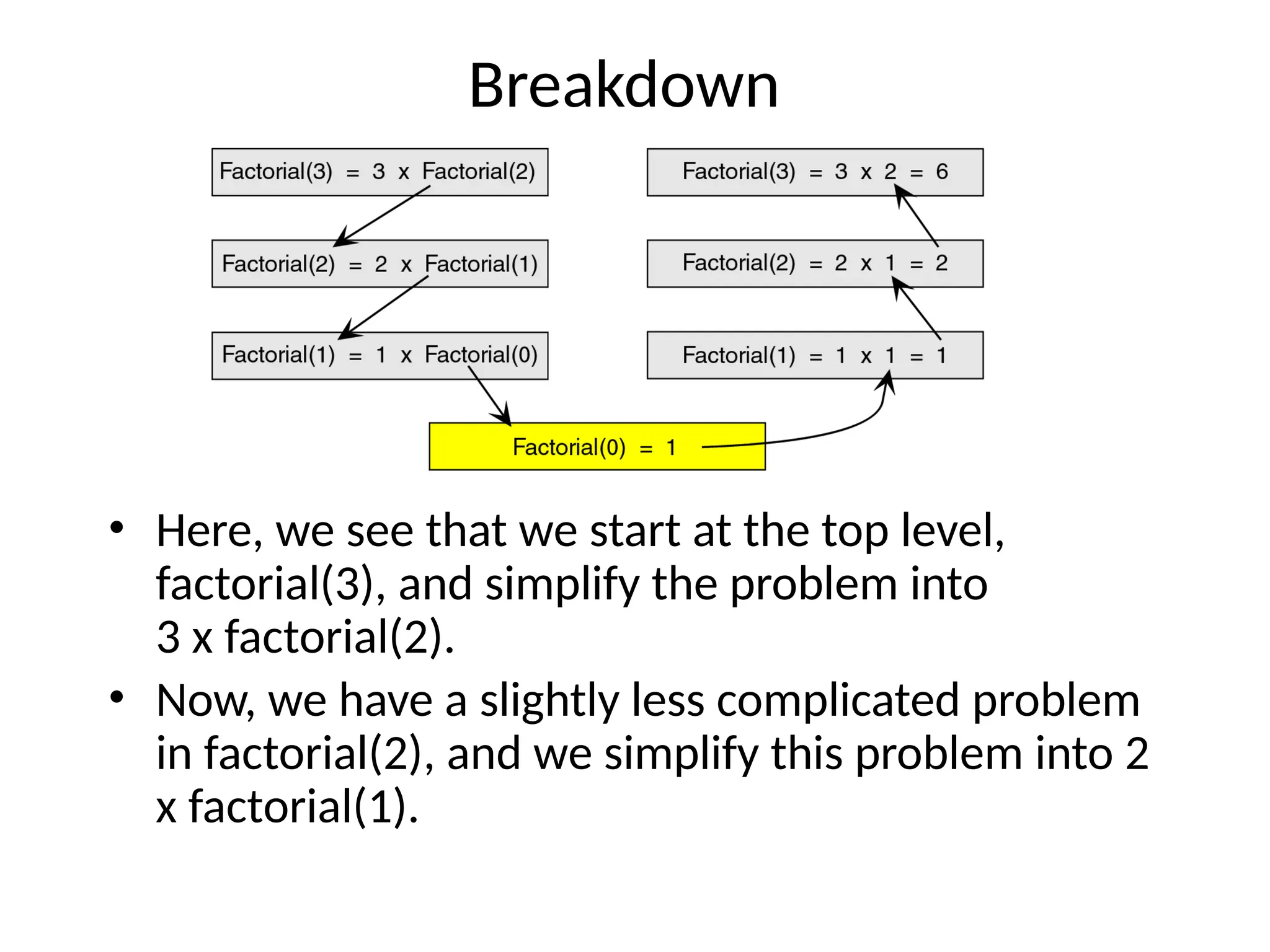
Recursion • To seehow the recursion works, let’s break down the factorial function to solve factorial(3)
11.
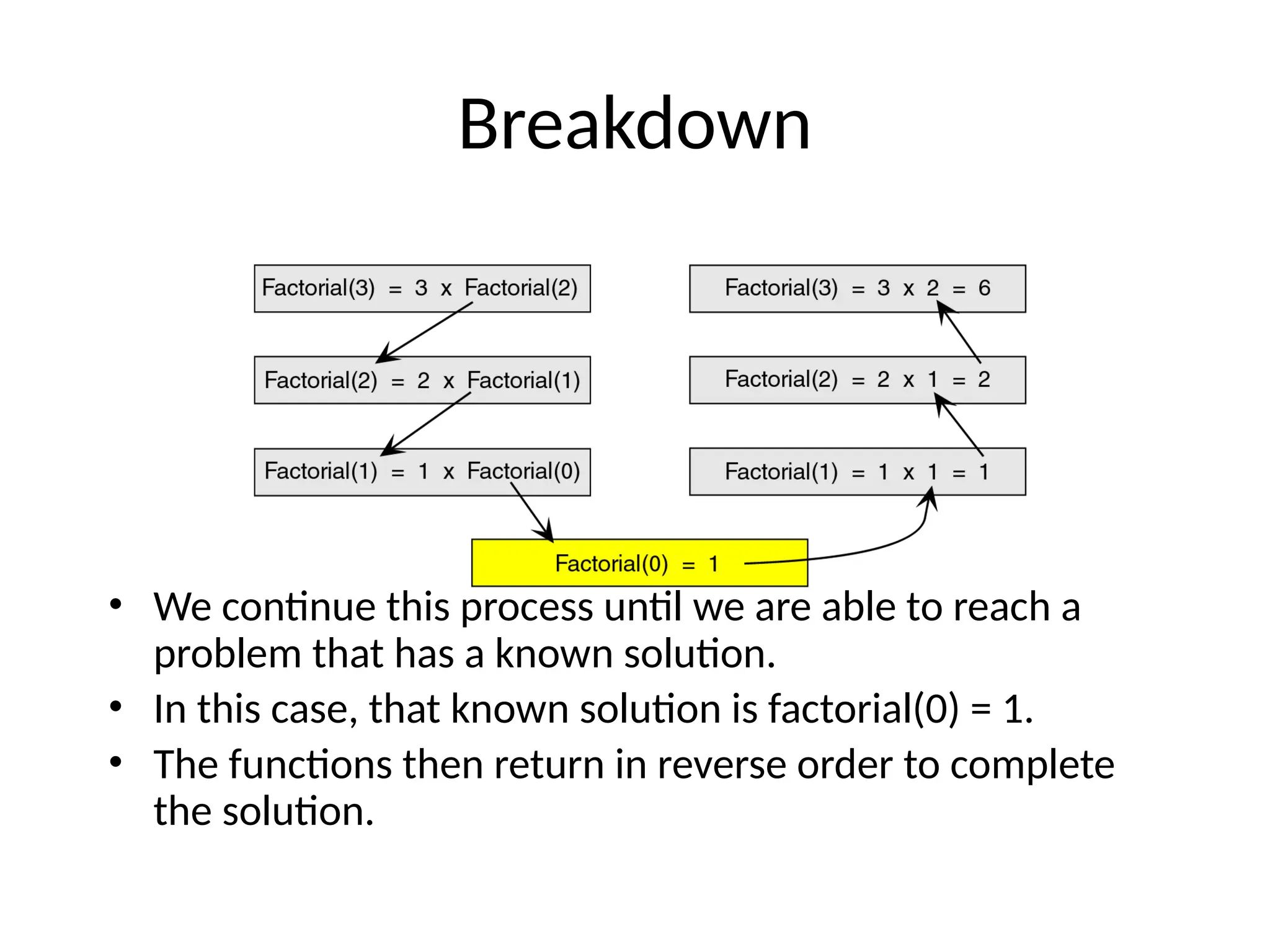
Breakdown • Here, wesee that we start at the top level, factorial(3), and simplify the problem into 3 x factorial(2). • Now, we have a slightly less complicated problem in factorial(2), and we simplify this problem into 2 x factorial(1).
12.
Breakdown • We continuethis process until we are able to reach a problem that has a known solution. • In this case, that known solution is factorial(0) = 1. • The functions then return in reverse order to complete the solution.
13.
Breakdown • This knownsolution is called the base case. • Every recursive algorithm must have a base case to simplify to. • Otherwise, the algorithm would run forever (or until the computer ran out of memory).
14.
Breakdown • The otherparts of the algorithm, excluding the base case, are known as the general case. • For example: 3 x factorial(2) general case 2 x factorial(1) general case etc …
15.
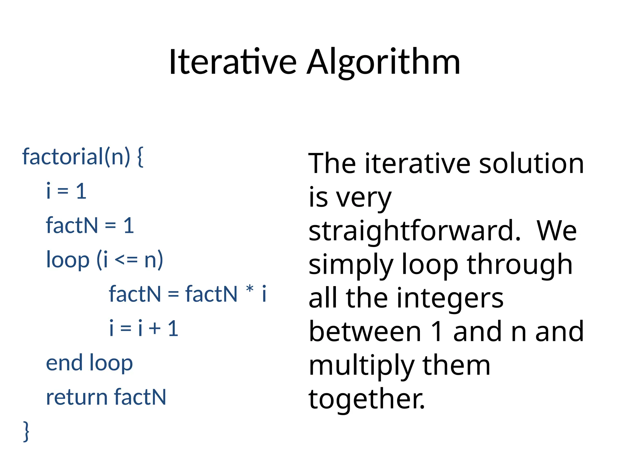
Iteration vs. Recursion •Now that we know the difference between an iterative algorithm and a recursive algorithm, we will develop both an iterative and a recursive algorithm to calculate the factorial of a number. • We will then compare the 2 algorithms.
16.
Iterative Algorithm factorial(n) { i= 1 factN = 1 loop (i <= n) factN = factN * i i = i + 1 end loop return factN } The iterative solution is very straightforward. We simply loop through all the integers between 1 and n and multiply them together.
17.
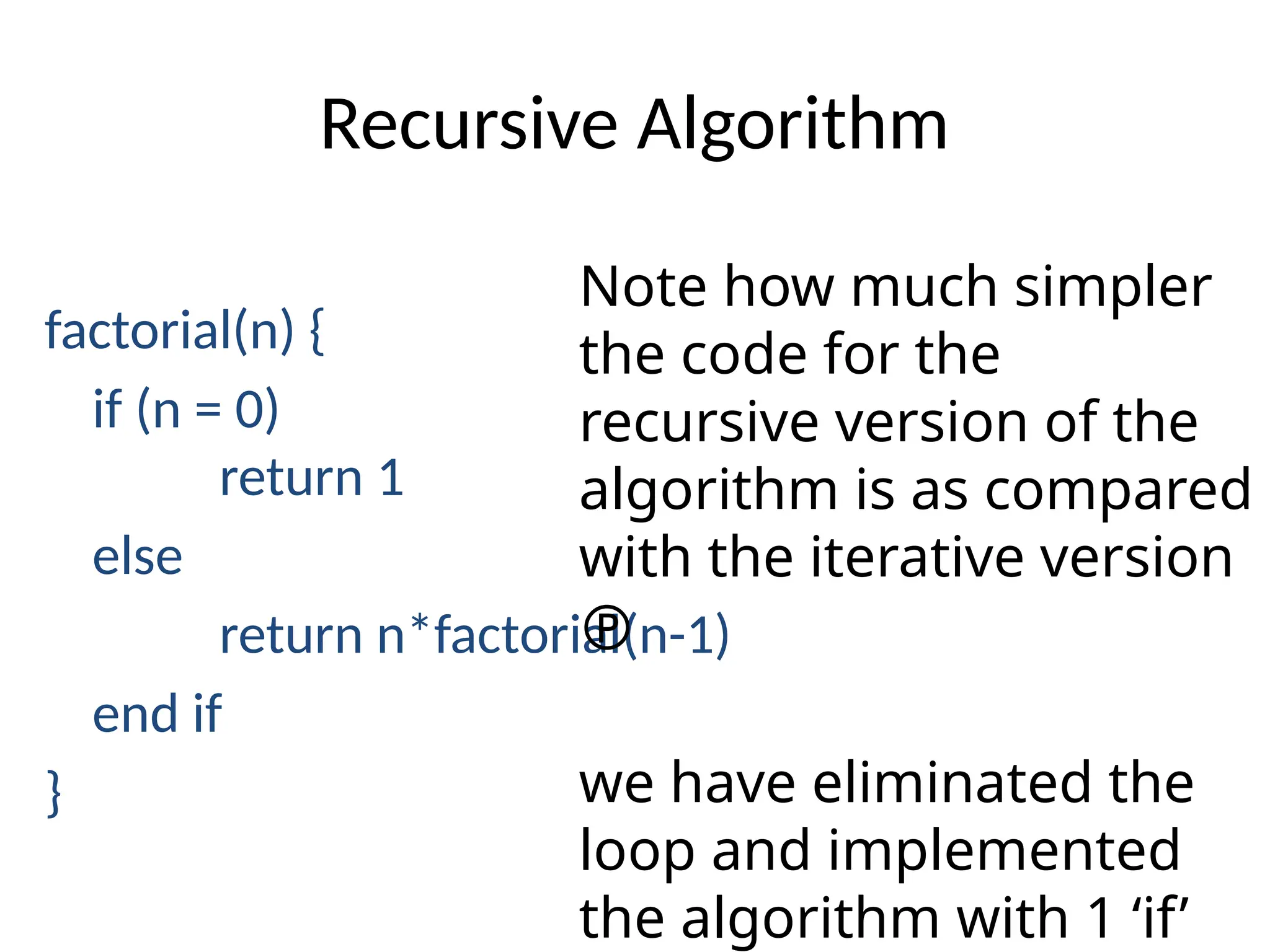
Recursive Algorithm factorial(n) { if(n = 0) return 1 else return n*factorial(n-1) end if } Note how much simpler the code for the recursive version of the algorithm is as compared with the iterative version we have eliminated the loop and implemented the algorithm with 1 ‘if’
19.
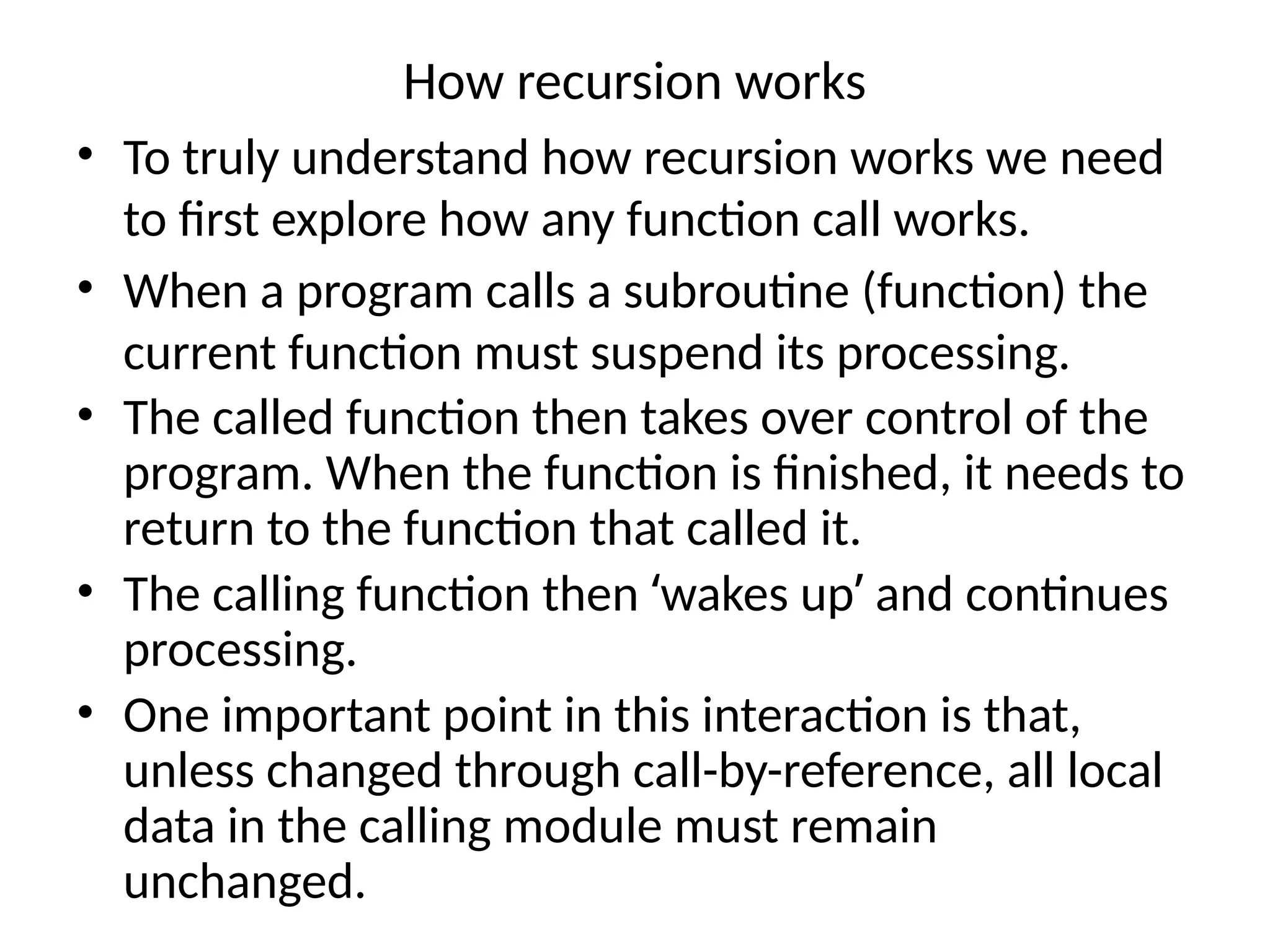
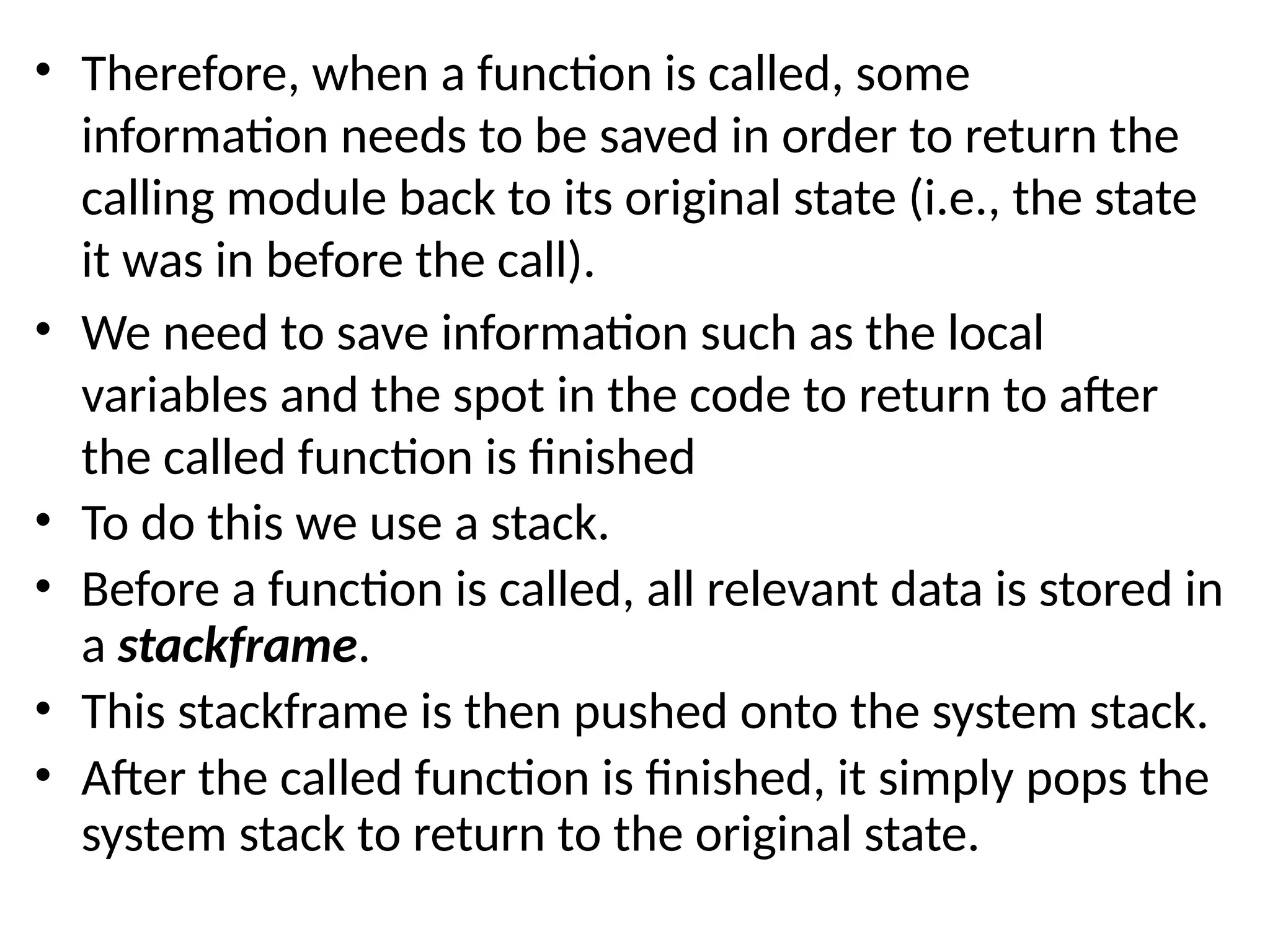
How recursion works •To truly understand how recursion works we need to first explore how any function call works. • When a program calls a subroutine (function) the current function must suspend its processing. • The called function then takes over control of the program. When the function is finished, it needs to return to the function that called it. • The calling function then ‘wakes up’ and continues processing. • One important point in this interaction is that, unless changed through call-by-reference, all local data in the calling module must remain unchanged.
20.
• Therefore, whena function is called, some information needs to be saved in order to return the calling module back to its original state (i.e., the state it was in before the call). • We need to save information such as the local variables and the spot in the code to return to after the called function is finished • To do this we use a stack. • Before a function is called, all relevant data is stored in a stackframe. • This stackframe is then pushed onto the system stack. • After the called function is finished, it simply pops the system stack to return to the original state.
21.
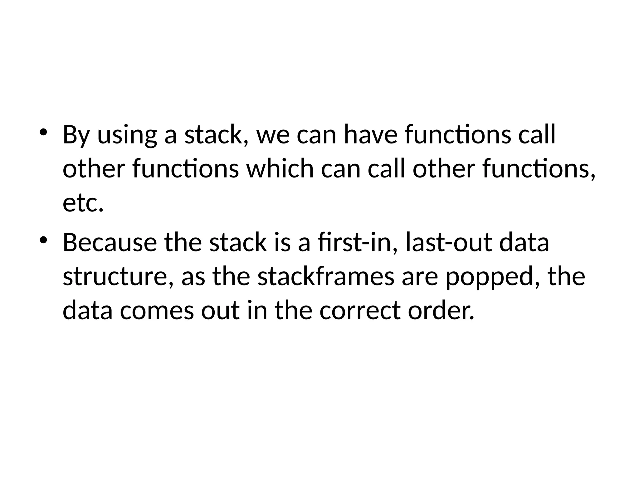
• By usinga stack, we can have functions call other functions which can call other functions, etc. • Because the stack is a first-in, last-out data structure, as the stackframes are popped, the data comes out in the correct order.
22.
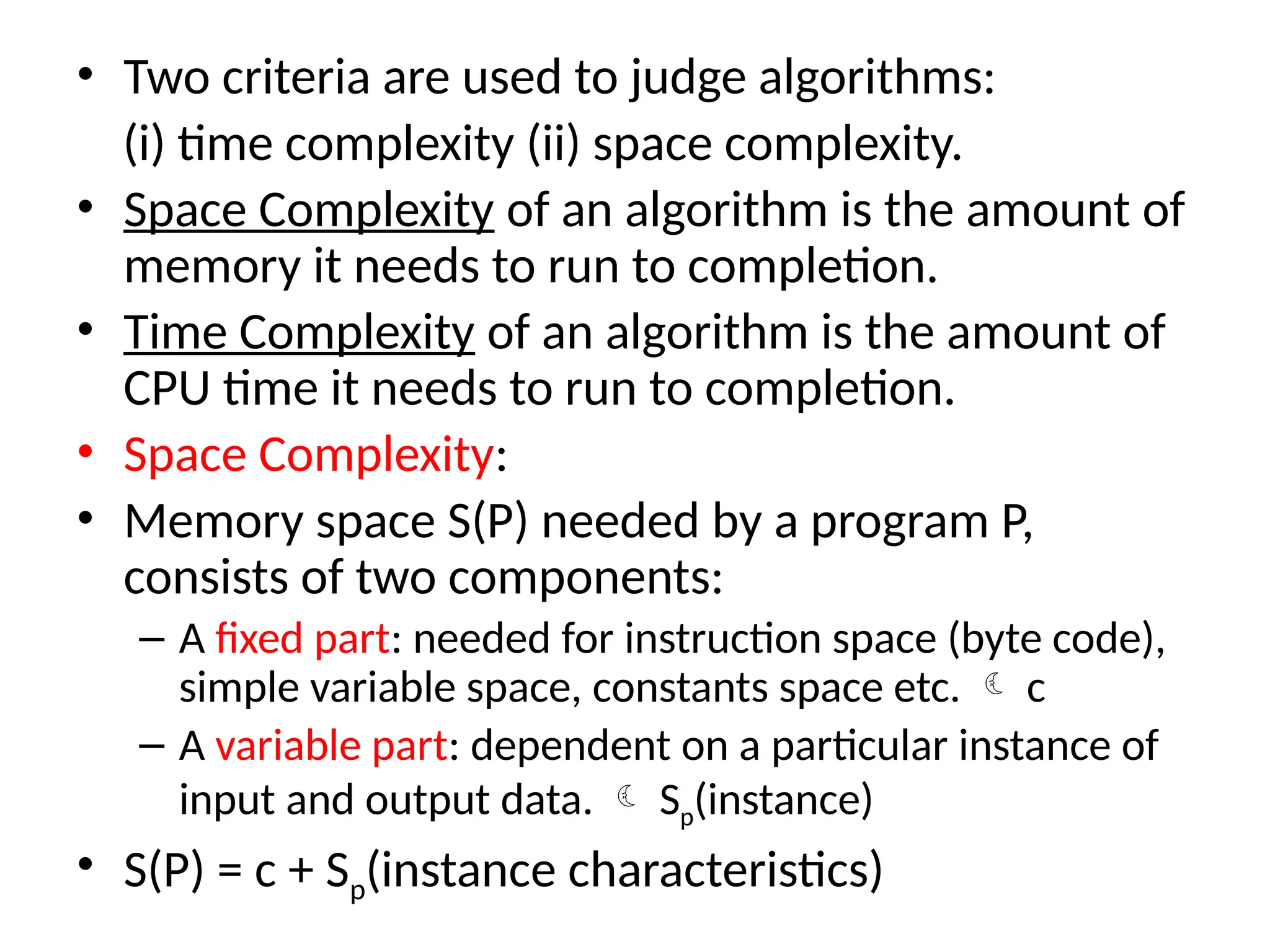
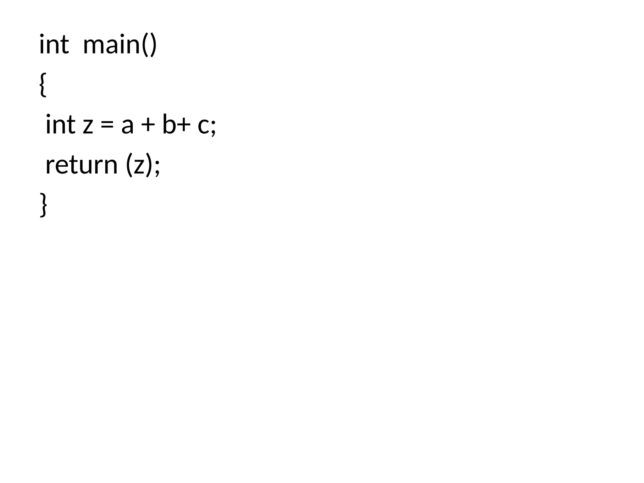
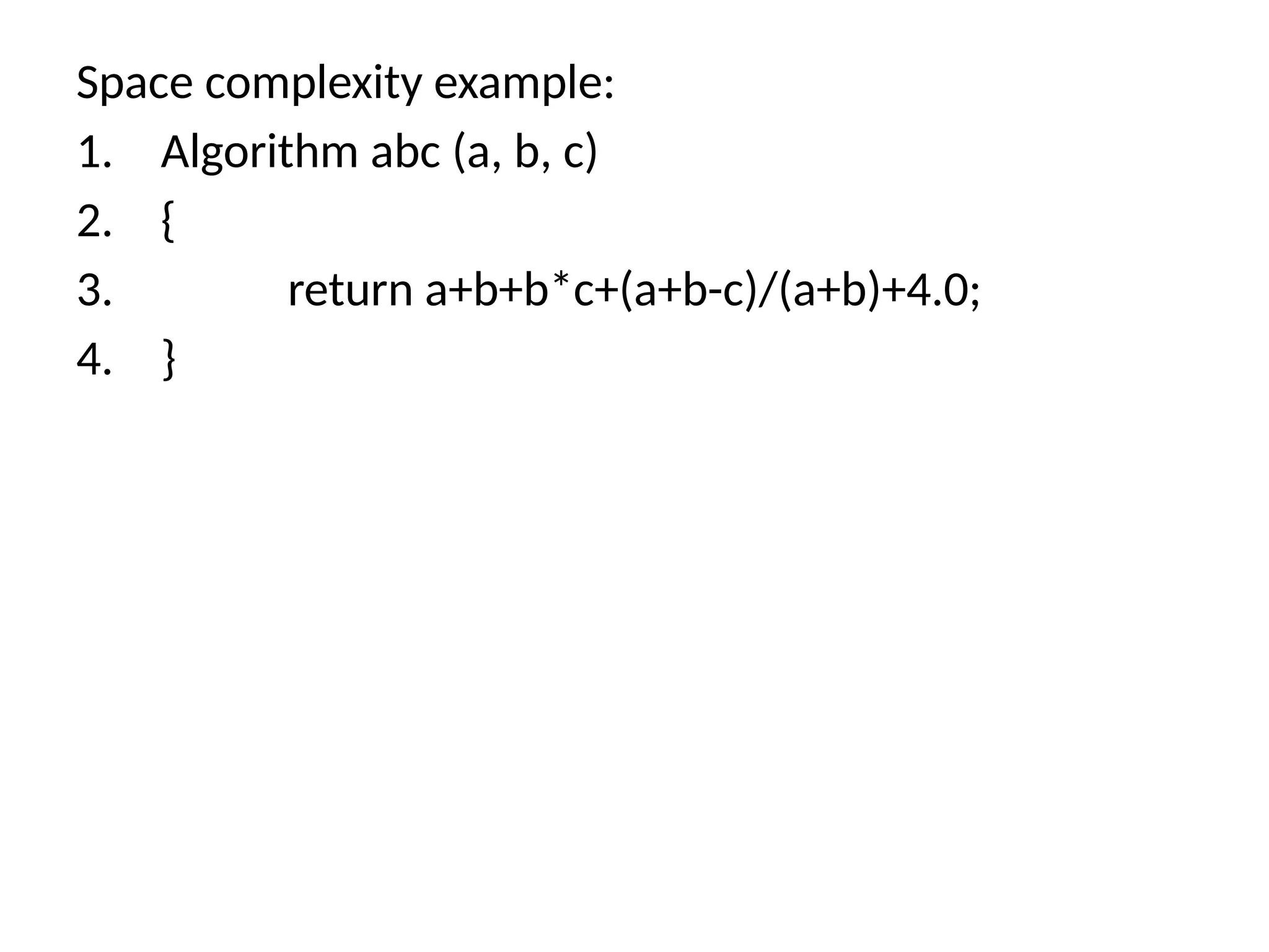
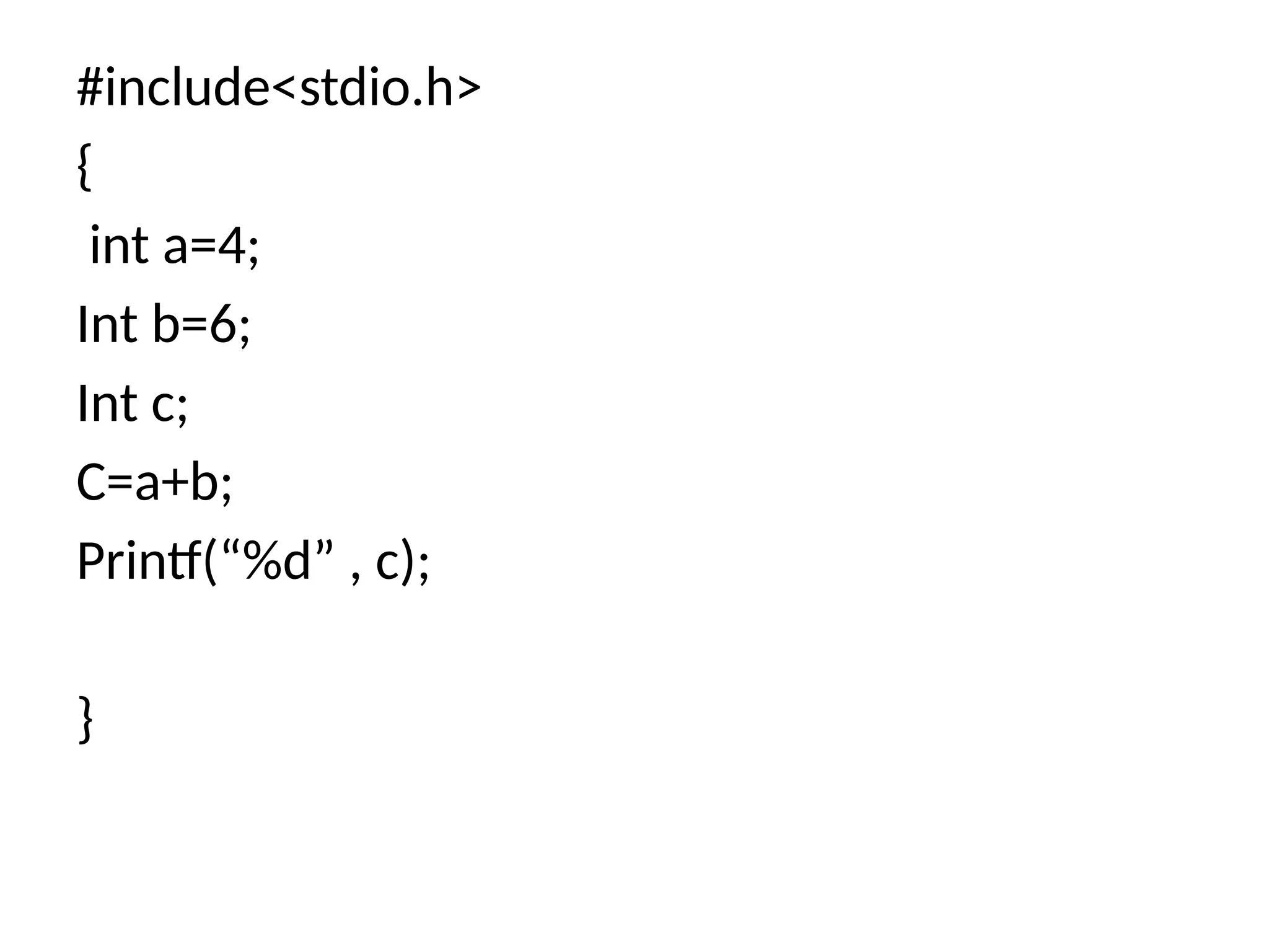
• Two criteriaare used to judge algorithms: (i) time complexity (ii) space complexity. • Space Complexity of an algorithm is the amount of memory it needs to run to completion. • Time Complexity of an algorithm is the amount of CPU time it needs to run to completion. • Space Complexity: • Memory space S(P) needed by a program P, consists of two components: – A fixed part: needed for instruction space (byte code), simple variable space, constants space etc. c – A variable part: dependent on a particular instance of input and output data. Sp(instance) • S(P) = c + Sp(instance characteristics)
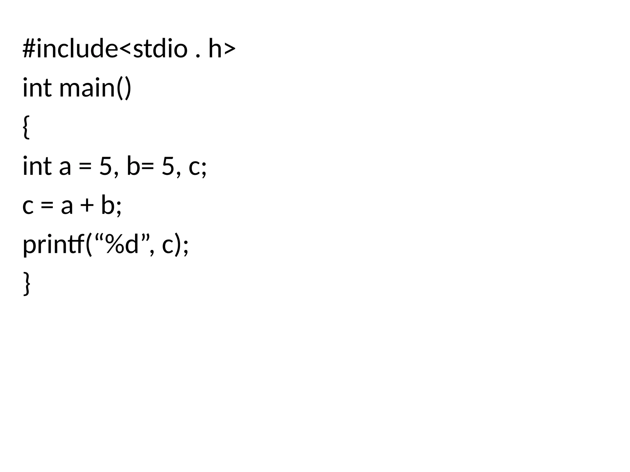
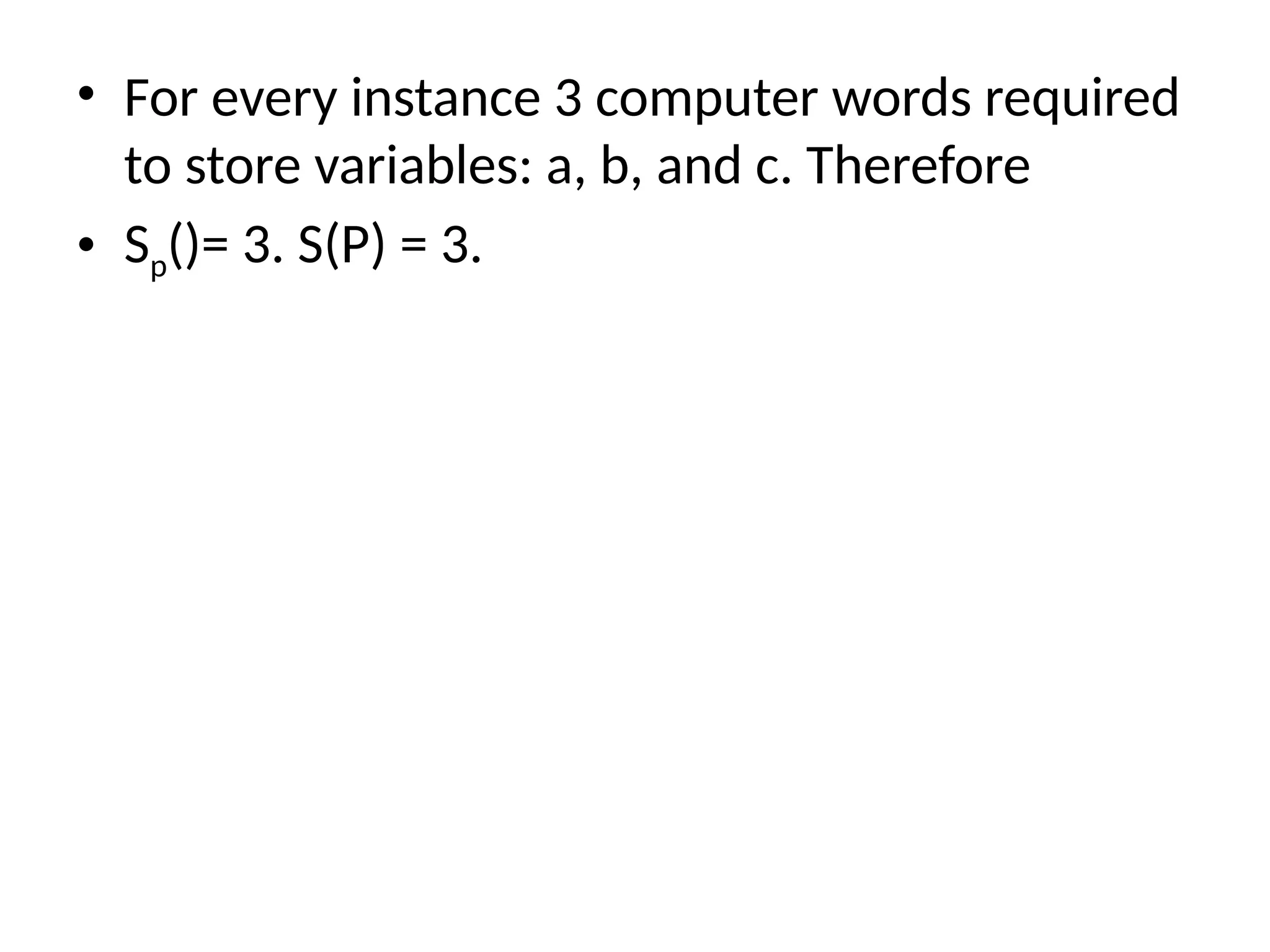
• For everyinstance 3 computer words required to store variables: a, b, and c. Therefore • Sp()= 3. S(P) = 3.
29.
1. Algorithm Sum(a[], n) 2. { 3. s:= 0.0; 4. for i = 1 to n do 5. s := s + a[i]; 6. return s; 7. }
30.
• Every instanceneeds to store array a[] & n. – Space needed to store n = 1 word. – Space needed to store a[ ] = n floating point words (or at least n words) – Space needed to store i and s = 2 words • Sp(n) = (n + 3). Hence S(P) = (n + 3).
31.
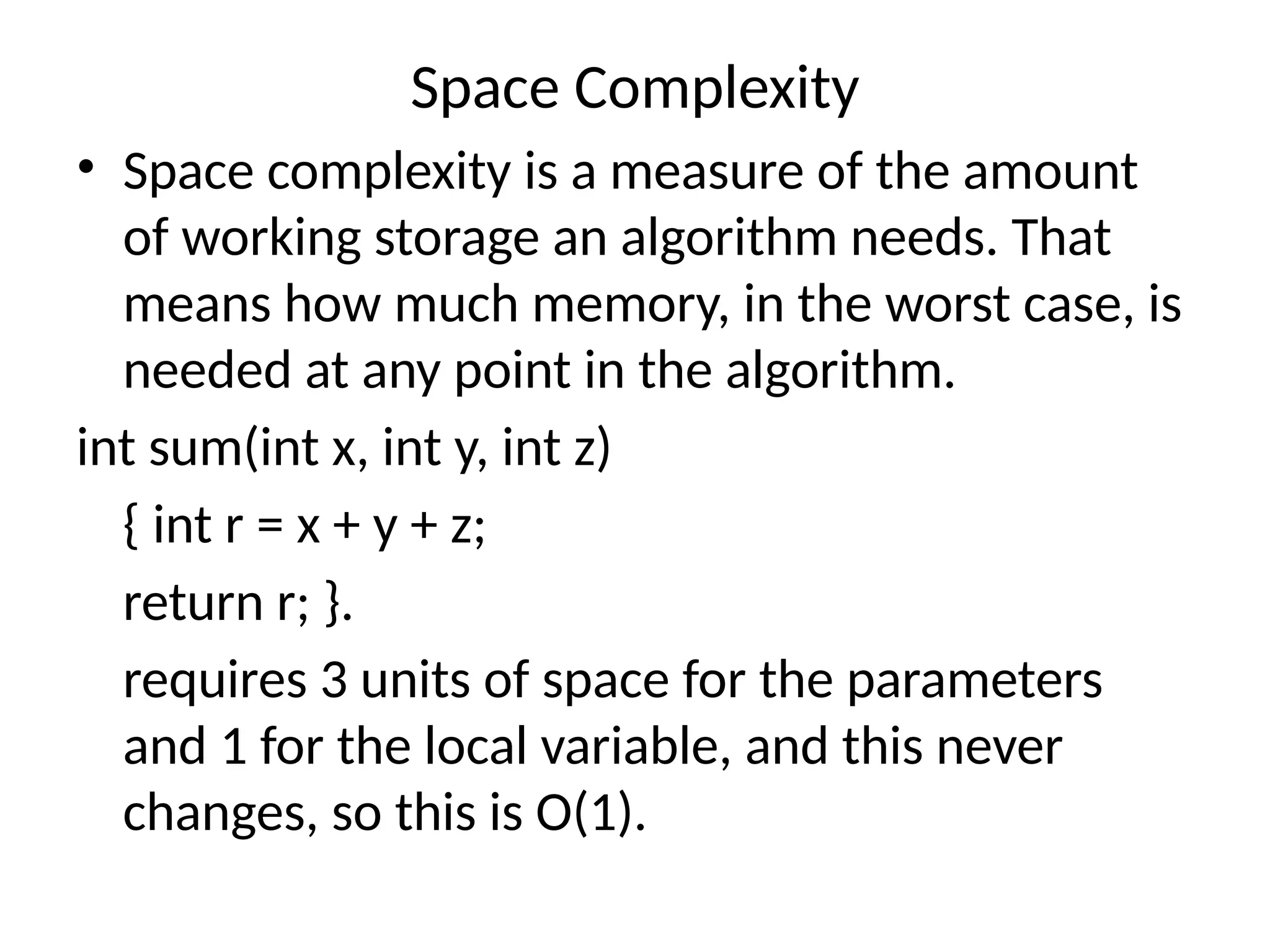
Space Complexity • Spacecomplexity is a measure of the amount of working storage an algorithm needs. That means how much memory, in the worst case, is needed at any point in the algorithm. int sum(int x, int y, int z) { int r = x + y + z; return r; }. requires 3 units of space for the parameters and 1 for the local variable, and this never changes, so this is O(1).
32.
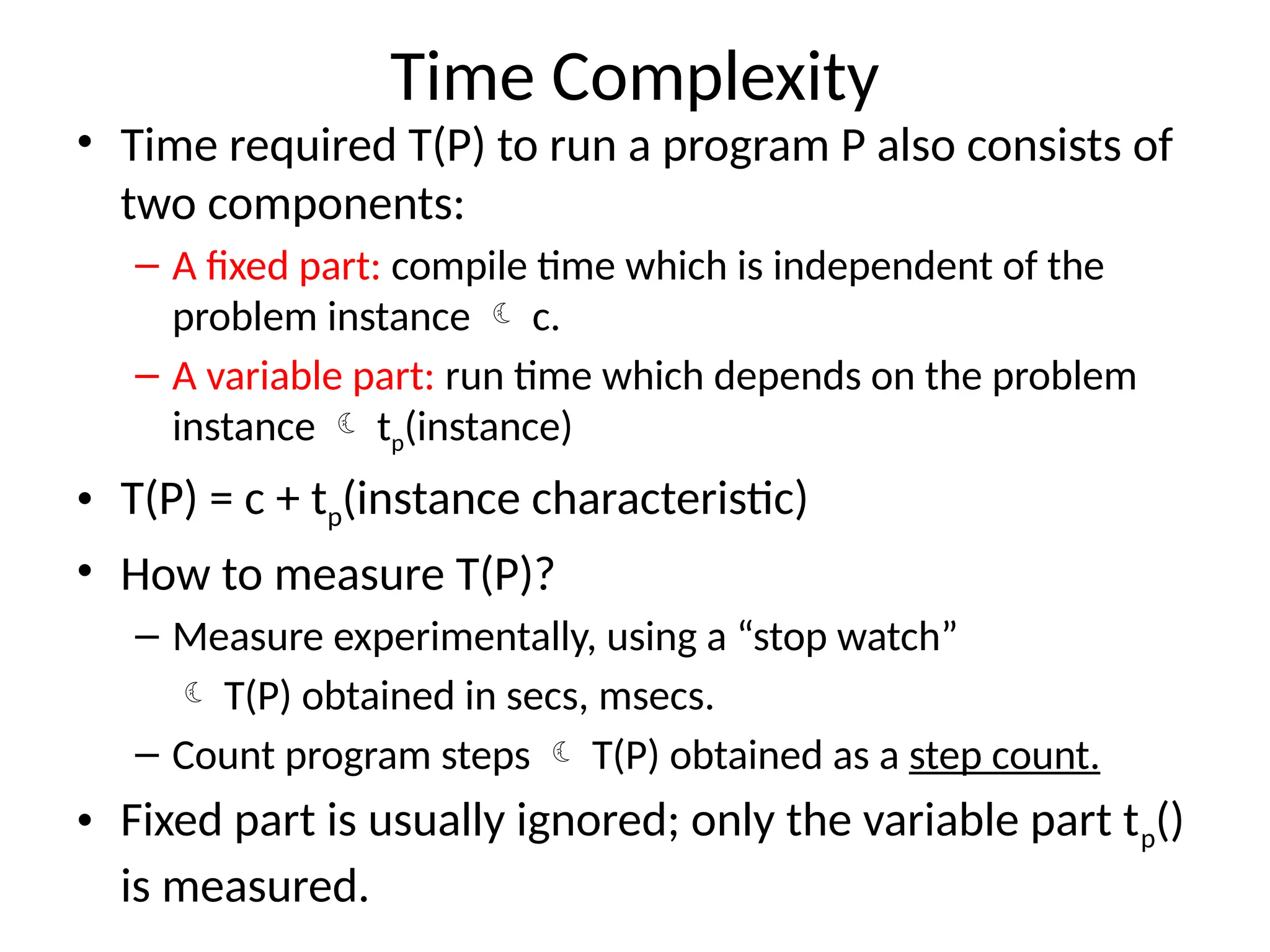
Time Complexity • Timerequired T(P) to run a program P also consists of two components: – A fixed part: compile time which is independent of the problem instance c. – A variable part: run time which depends on the problem instance tp(instance) • T(P) = c + tp(instance characteristic) • How to measure T(P)? – Measure experimentally, using a “stop watch” T(P) obtained in secs, msecs. – Count program steps T(P) obtained as a step count. • Fixed part is usually ignored; only the variable part tp() is measured.
33.
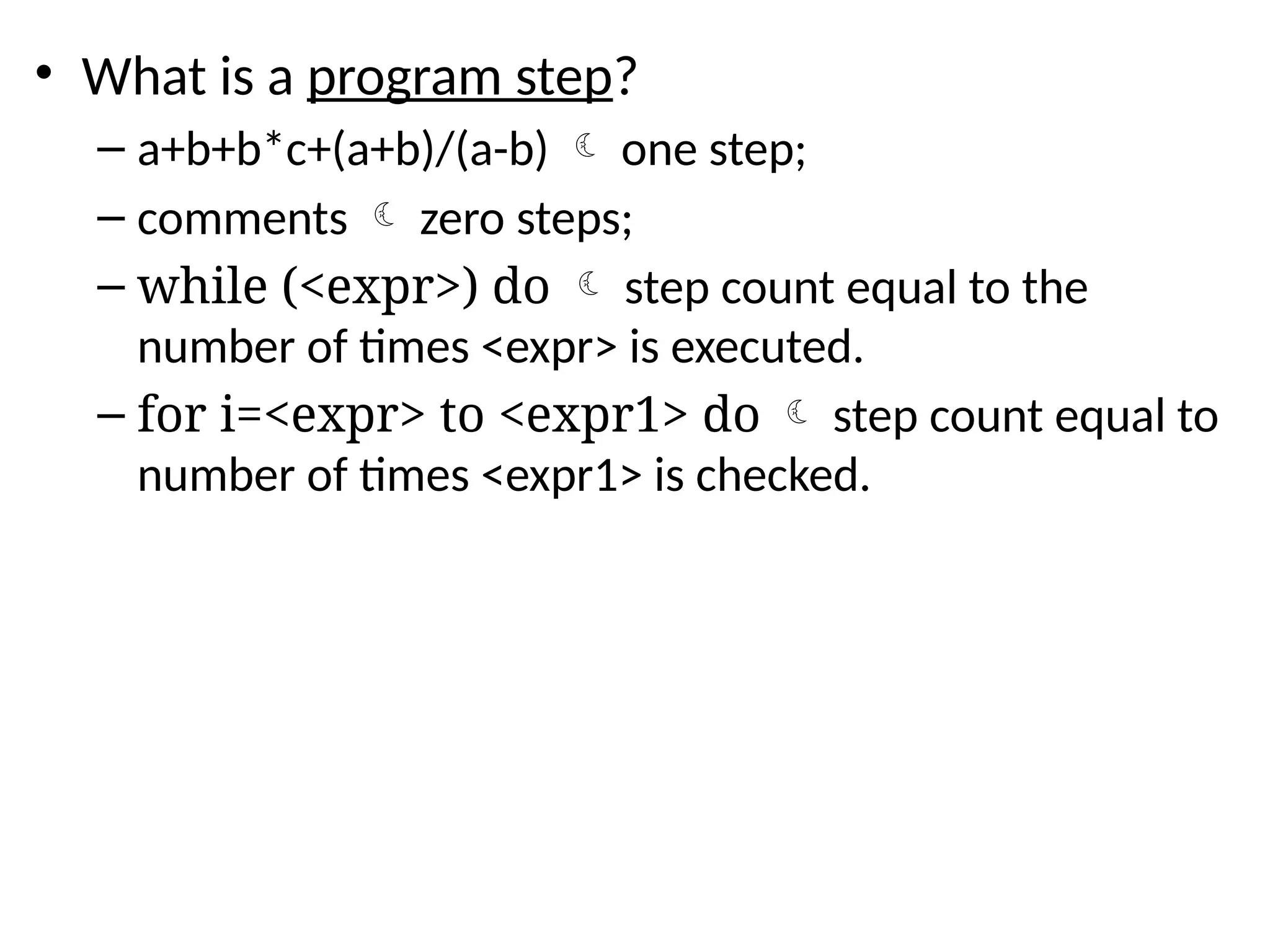
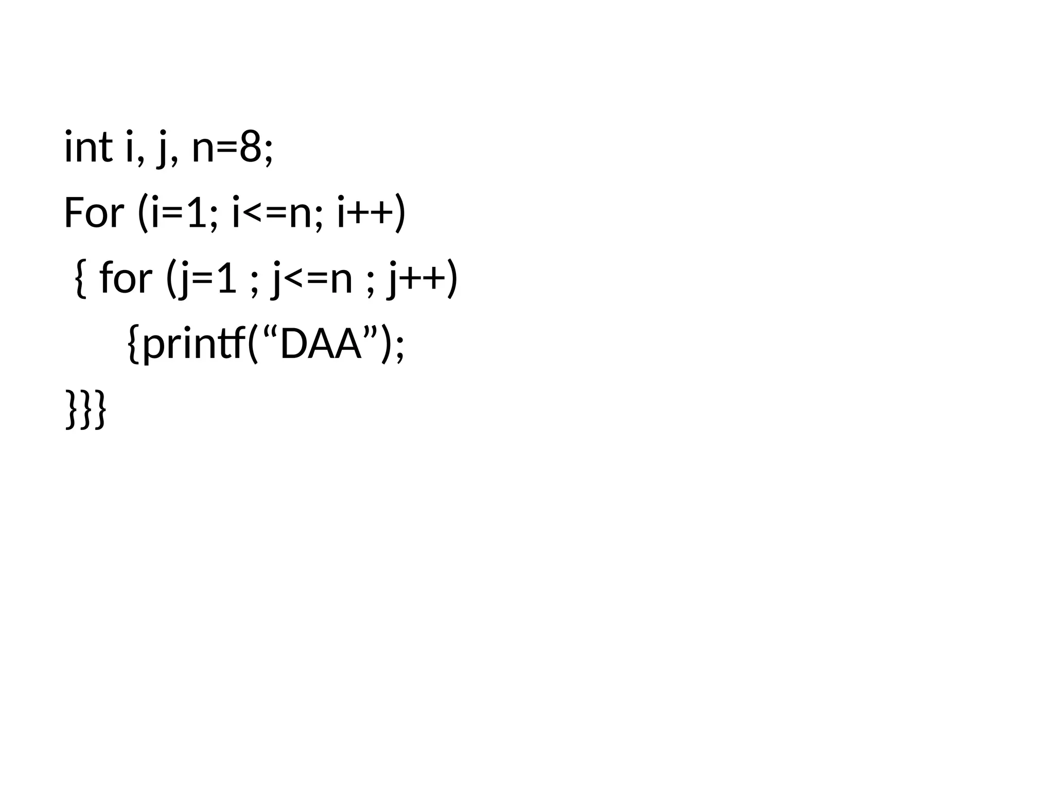
• What isa program step? – a+b+b*c+(a+b)/(a-b) one step; – comments zero steps; – while (<expr>) do step count equal to the number of times <expr> is executed. – for i=<expr> to <expr1> do step count equal to number of times <expr1> is checked.
int i, j,n=8; For (i=1; i<=n; i++) { for (j=1 ; j<=n ; j++) {printf(“DAA”); }}}
41.
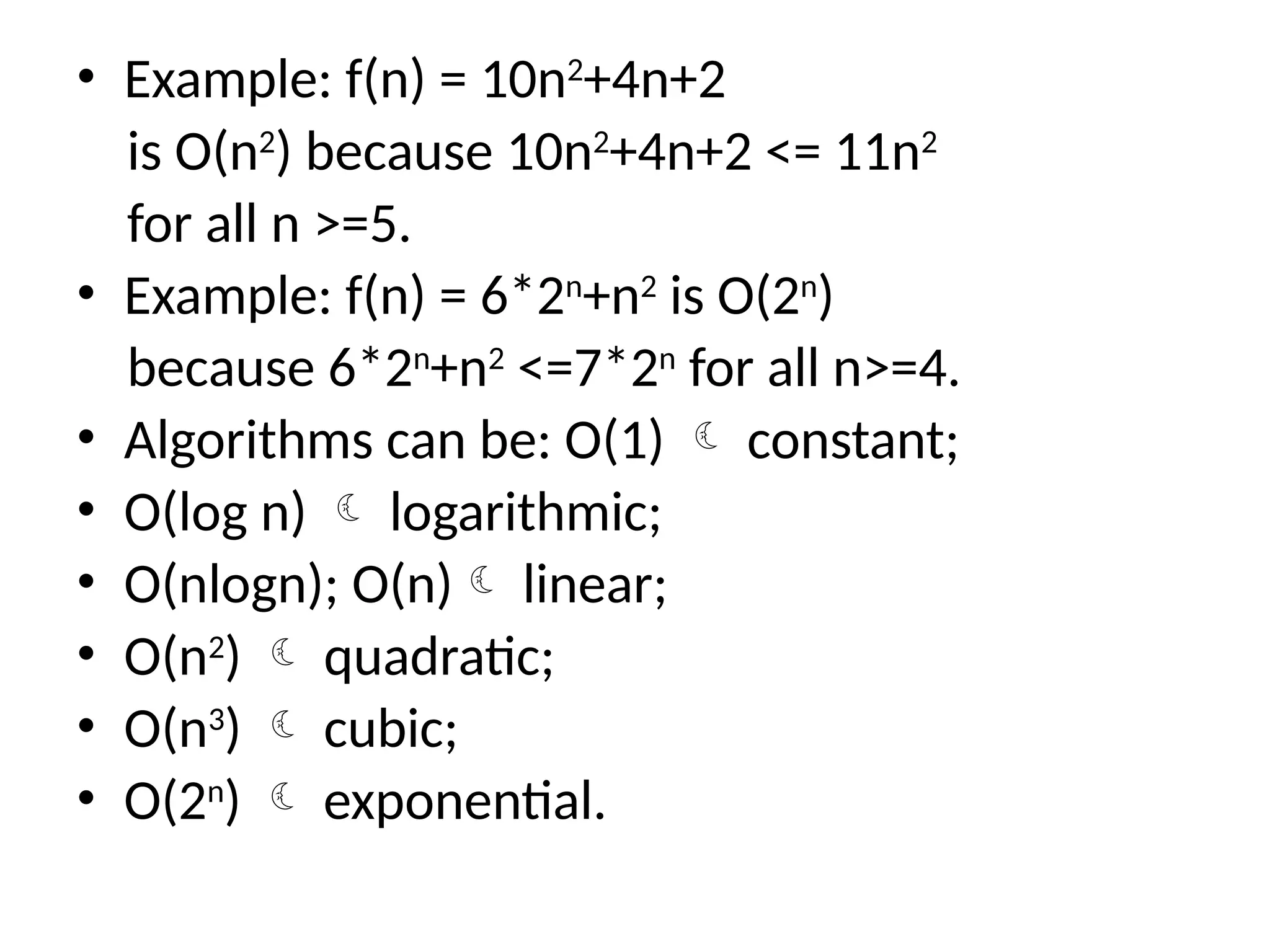
• Example: f(n)= 10n2 +4n+2 is O(n2 ) because 10n2 +4n+2 <= 11n2 for all n >=5. • Example: f(n) = 6*2n +n2 is O(2n ) because 6*2n +n2 <=7*2n for all n>=4. • Algorithms can be: O(1) constant; • O(log n) logarithmic; • O(nlogn); O(n) linear; • O(n2 ) quadratic; • O(n3 ) cubic; • O(2n ) exponential.
42.
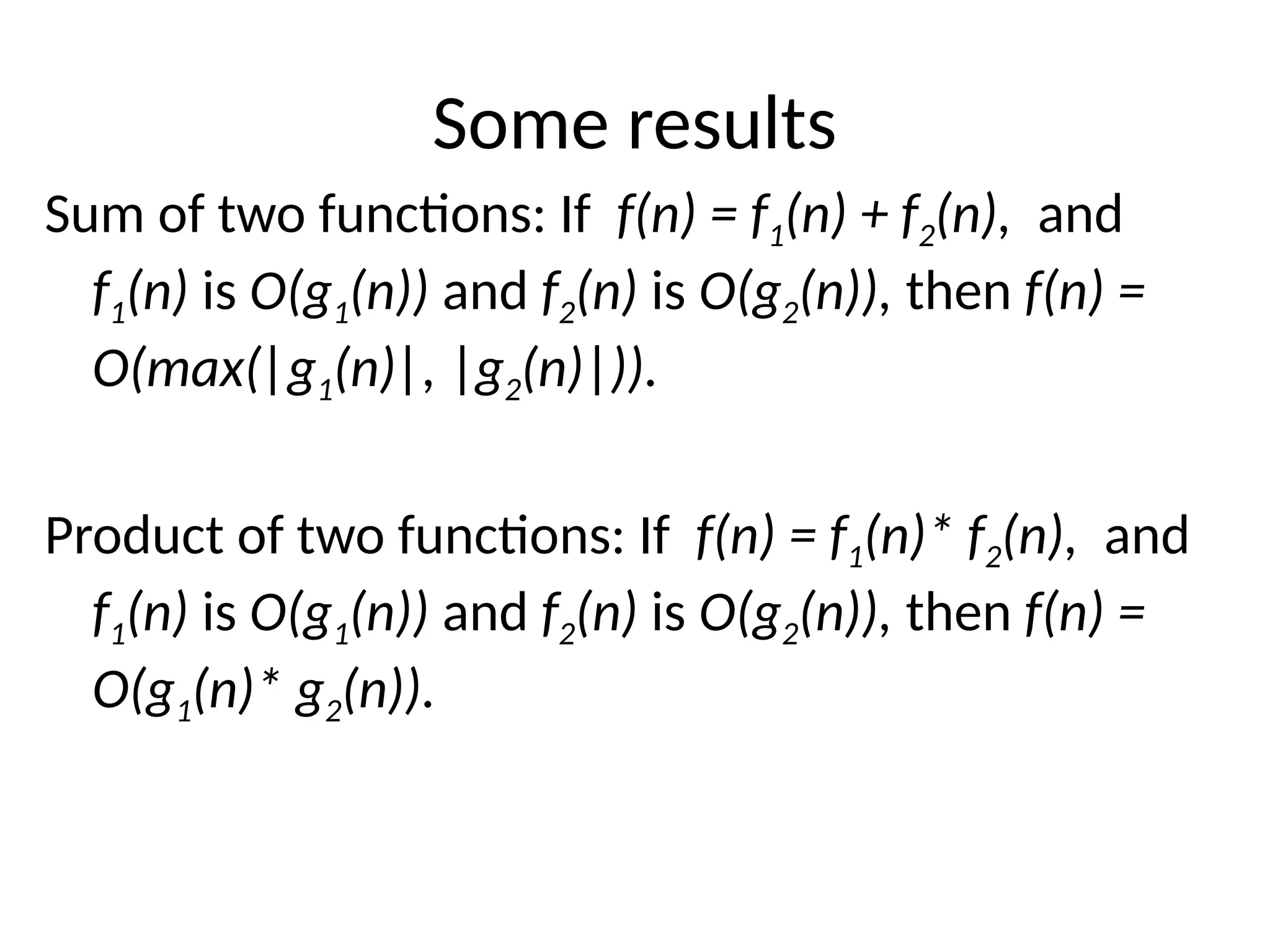
Some results Sum oftwo functions: If f(n) = f1(n) + f2(n), and f1(n) is O(g1(n)) and f2(n) is O(g2(n)), then f(n) = O(max(|g1(n)|, |g2(n)|)). Product of two functions: If f(n) = f1(n)* f2(n), and f1(n) is O(g1(n)) and f2(n) is O(g2(n)), then f(n) = O(g1(n)* g2(n)).
43.
int sum(int a[],int n) { int r = 0; for (int i = 0; i < n; ++i) { r += a[i]; } return r; } requires N units for a, plus space for n, r and i, so it's O(N).
44.
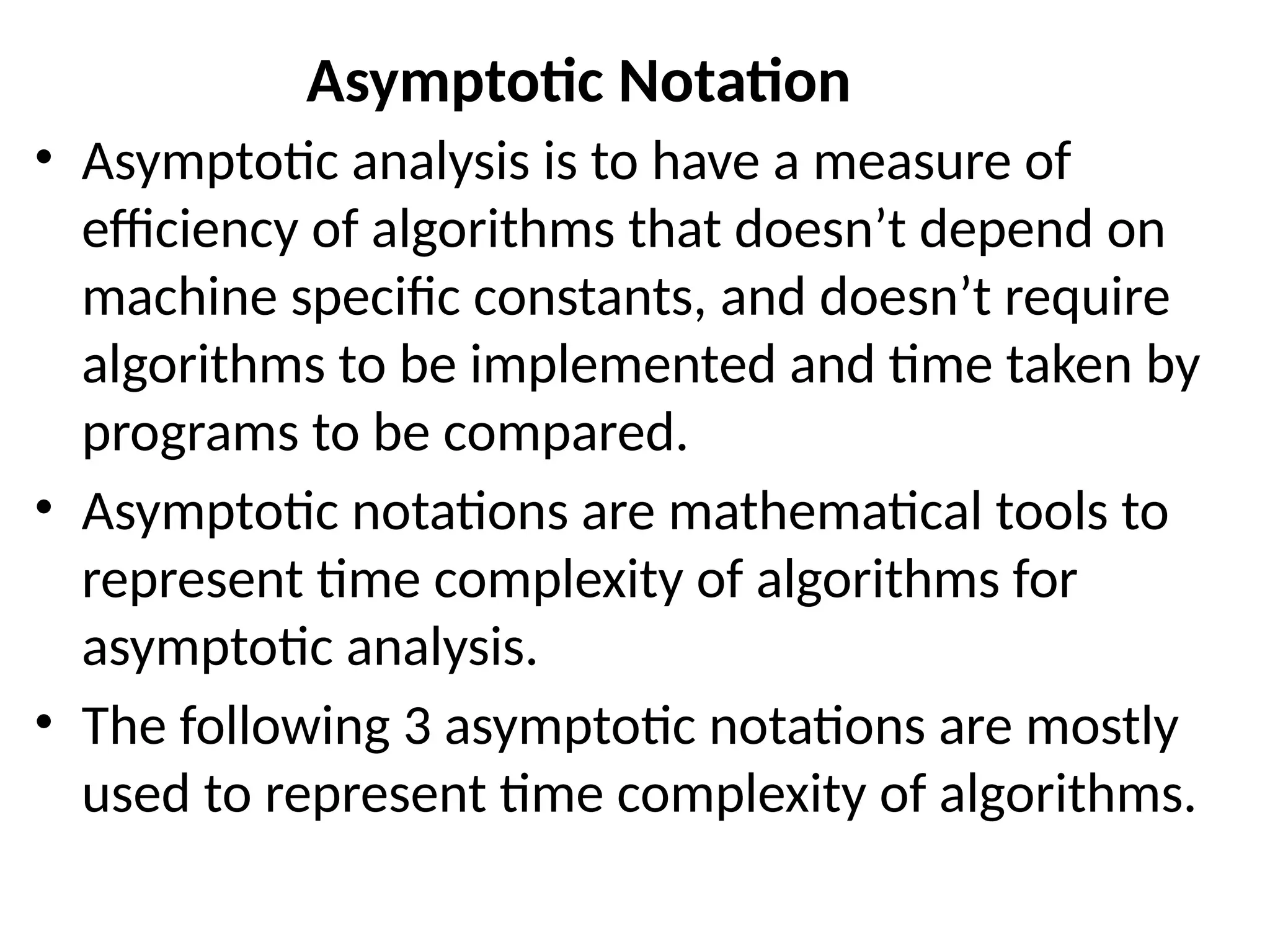
• Asymptotic analysisis to have a measure of efficiency of algorithms that doesn’t depend on machine specific constants, and doesn’t require algorithms to be implemented and time taken by programs to be compared. • Asymptotic notations are mathematical tools to represent time complexity of algorithms for asymptotic analysis. • The following 3 asymptotic notations are mostly used to represent time complexity of algorithms. Asymptotic Notation
45.
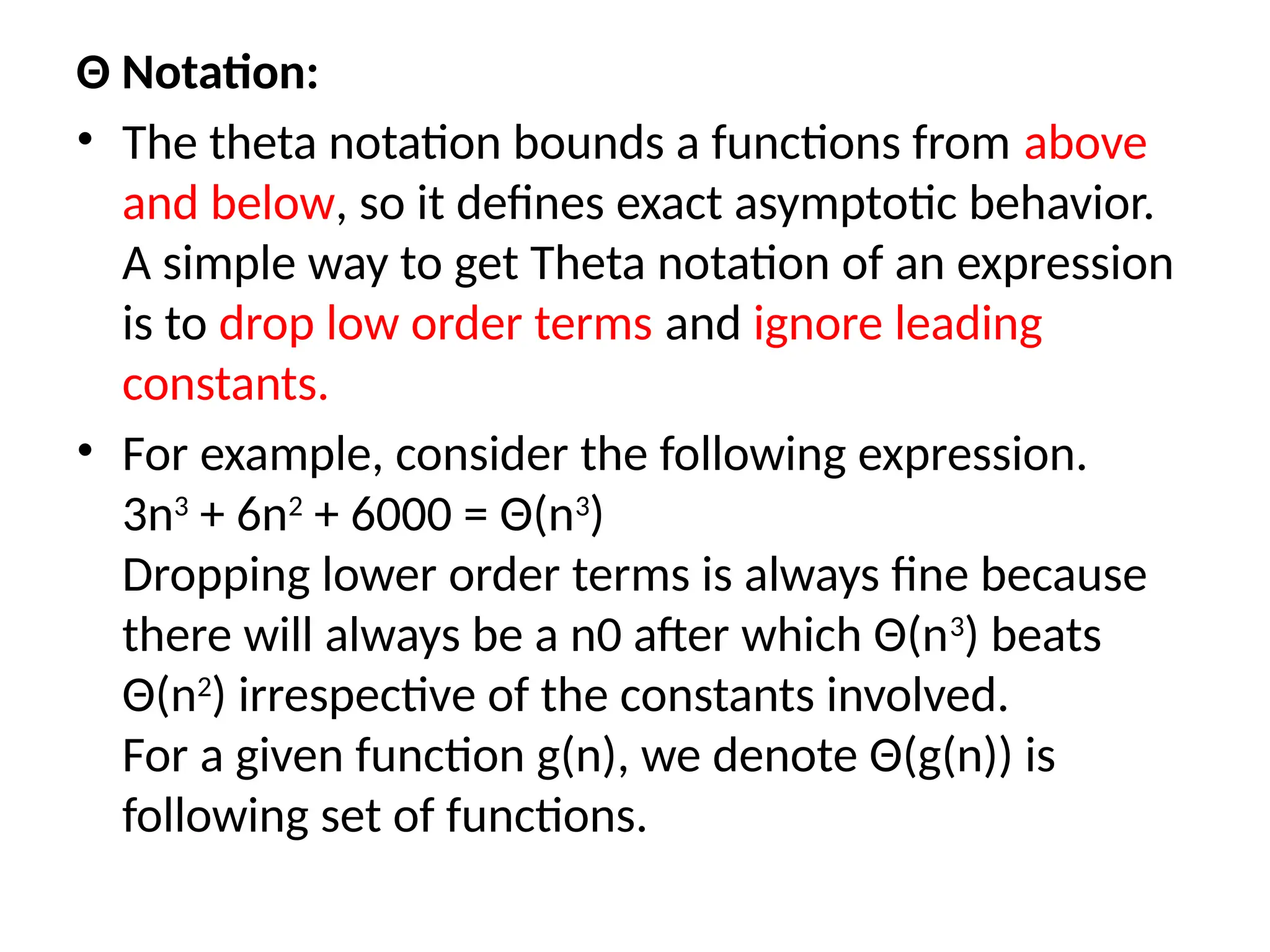
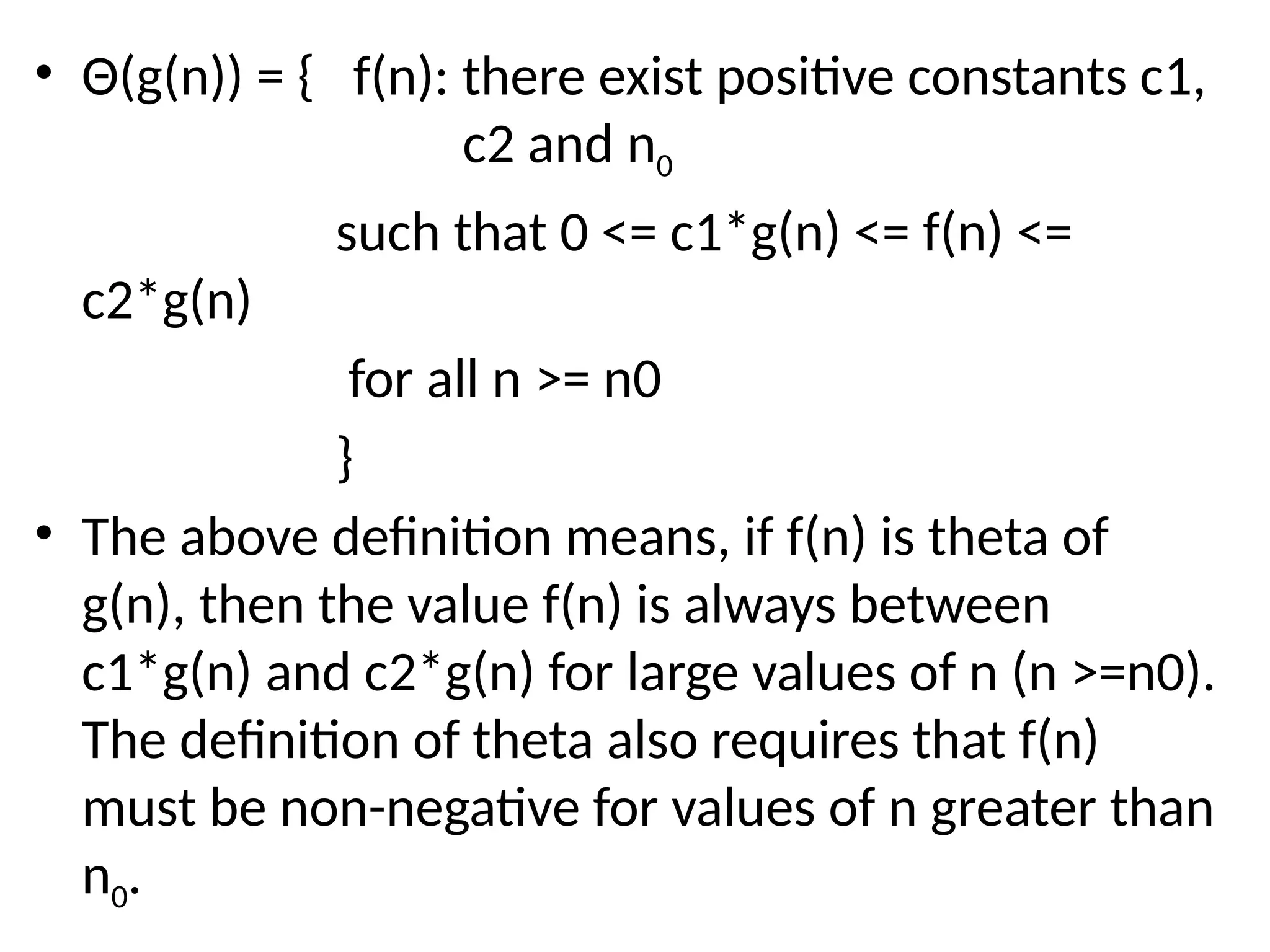
Θ Notation: • Thetheta notation bounds a functions from above and below, so it defines exact asymptotic behavior. A simple way to get Theta notation of an expression is to drop low order terms and ignore leading constants. • For example, consider the following expression. 3n3 + 6n2 + 6000 = Θ(n3 ) Dropping lower order terms is always fine because there will always be a n0 after which Θ(n3 ) beats Θ(n2 ) irrespective of the constants involved. For a given function g(n), we denote Θ(g(n)) is following set of functions.
47.
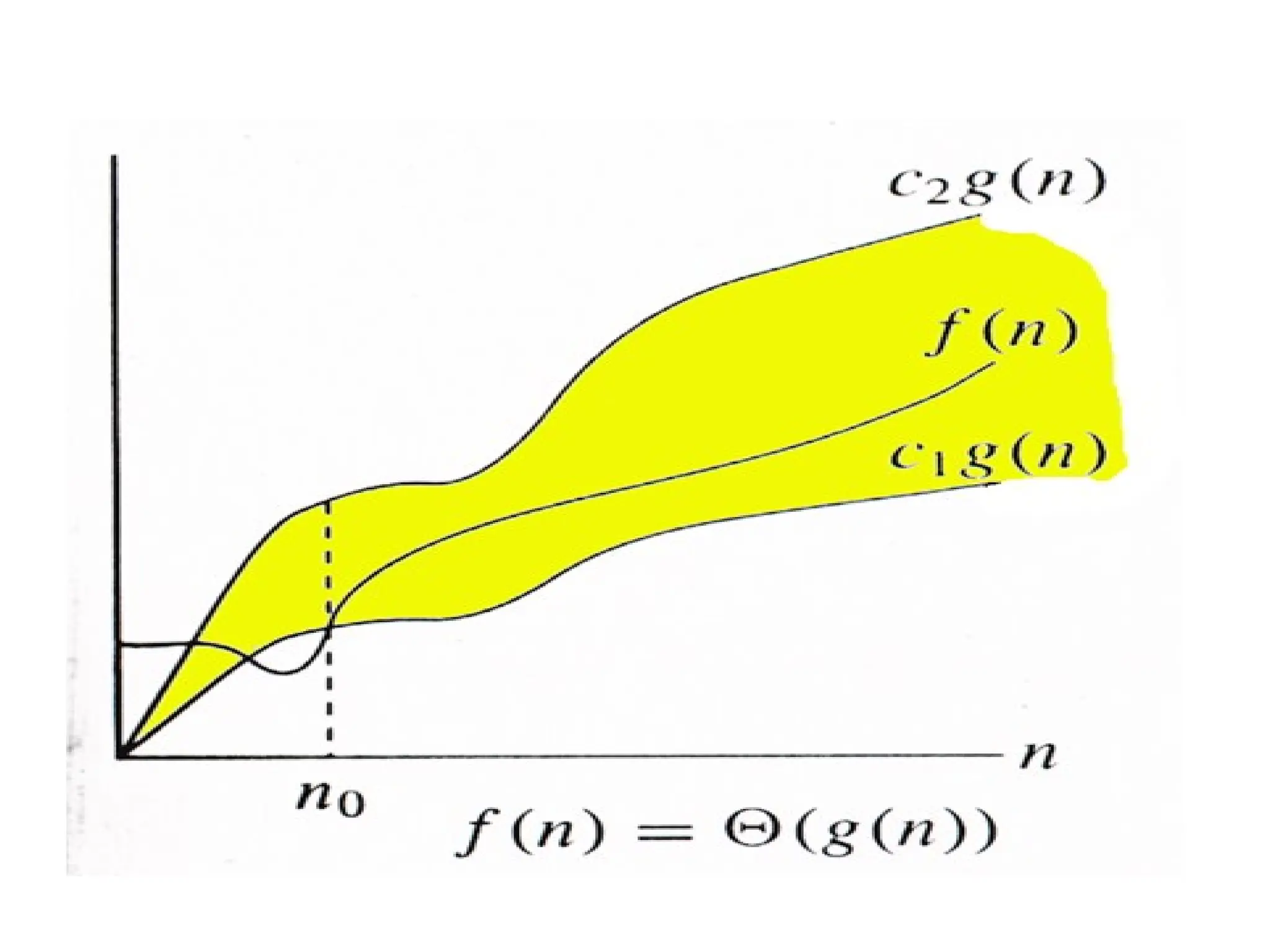
• Θ(g(n)) ={ f(n): there exist positive constants c1, c2 and n0 such that 0 <= c1*g(n) <= f(n) <= c2*g(n) for all n >= n0 } • The above definition means, if f(n) is theta of g(n), then the value f(n) is always between c1*g(n) and c2*g(n) for large values of n (n >=n0). The definition of theta also requires that f(n) must be non-negative for values of n greater than n0.
48.
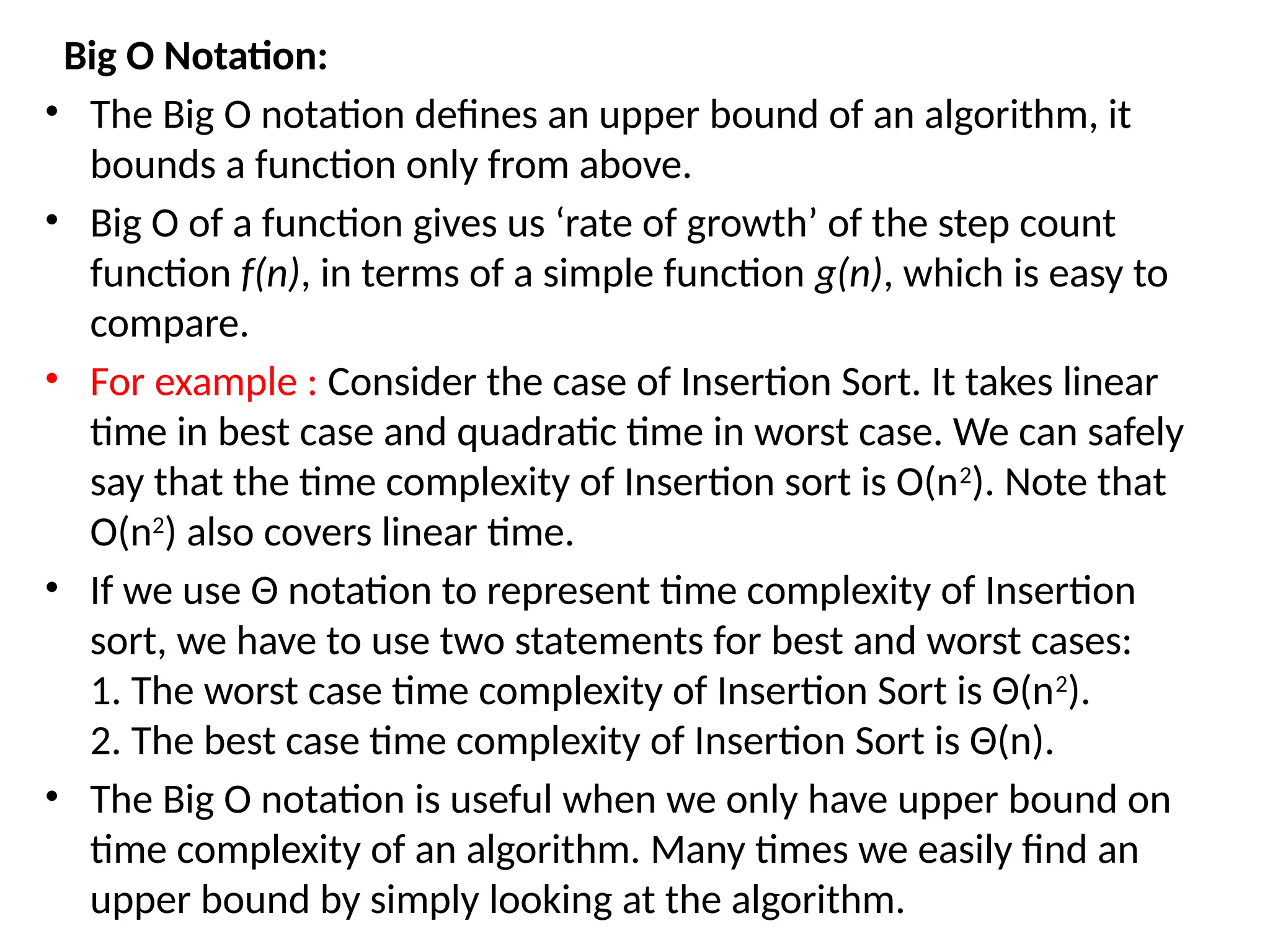
Big O Notation: •The Big O notation defines an upper bound of an algorithm, it bounds a function only from above. • Big O of a function gives us ‘rate of growth’ of the step count function f(n), in terms of a simple function g(n), which is easy to compare. • For example : Consider the case of Insertion Sort. It takes linear time in best case and quadratic time in worst case. We can safely say that the time complexity of Insertion sort is O(n2 ). Note that O(n2 ) also covers linear time. • If we use Θ notation to represent time complexity of Insertion sort, we have to use two statements for best and worst cases: 1. The worst case time complexity of Insertion Sort is Θ(n2 ). 2. The best case time complexity of Insertion Sort is Θ(n). • The Big O notation is useful when we only have upper bound on time complexity of an algorithm. Many times we easily find an upper bound by simply looking at the algorithm.
49.
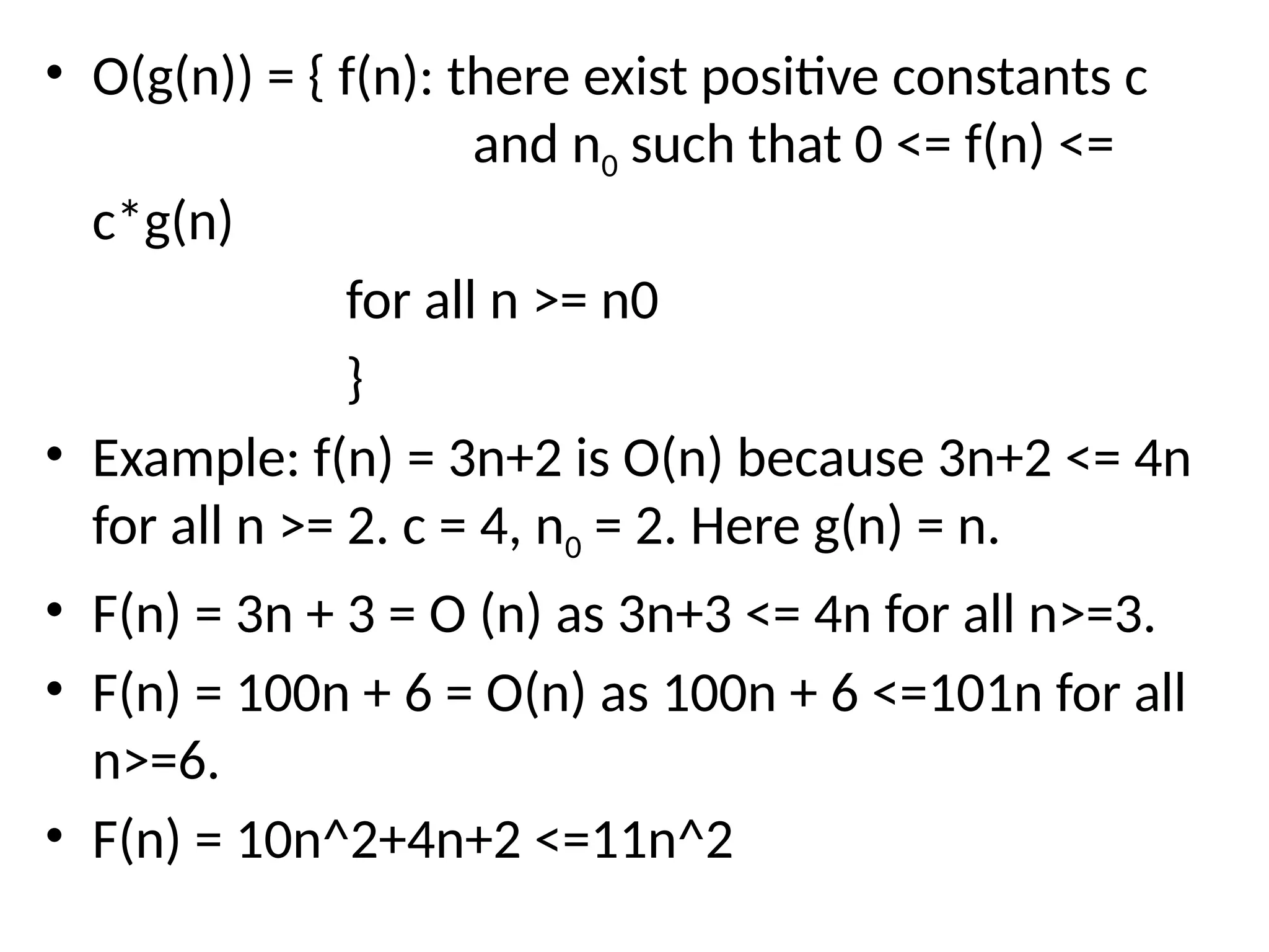
• O(g(n)) ={ f(n): there exist positive constants c and n0 such that 0 <= f(n) <= c*g(n) for all n >= n0 } • Example: f(n) = 3n+2 is O(n) because 3n+2 <= 4n for all n >= 2. c = 4, n0 = 2. Here g(n) = n. • F(n) = 3n + 3 = O (n) as 3n+3 <= 4n for all n>=3. • F(n) = 100n + 6 = O(n) as 100n + 6 <=101n for all n>=6. • F(n) = 10n^2+4n+2 <=11n^2
50.
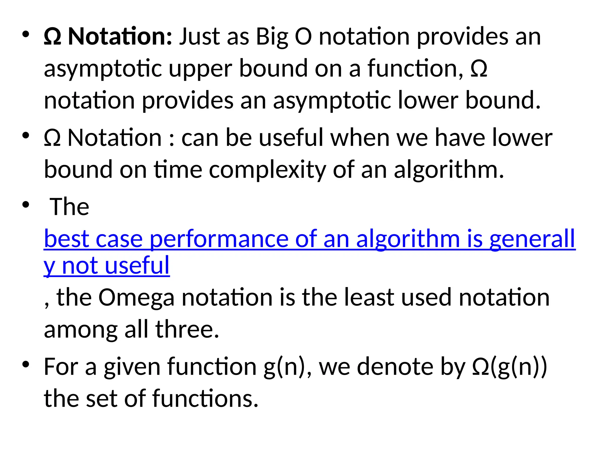
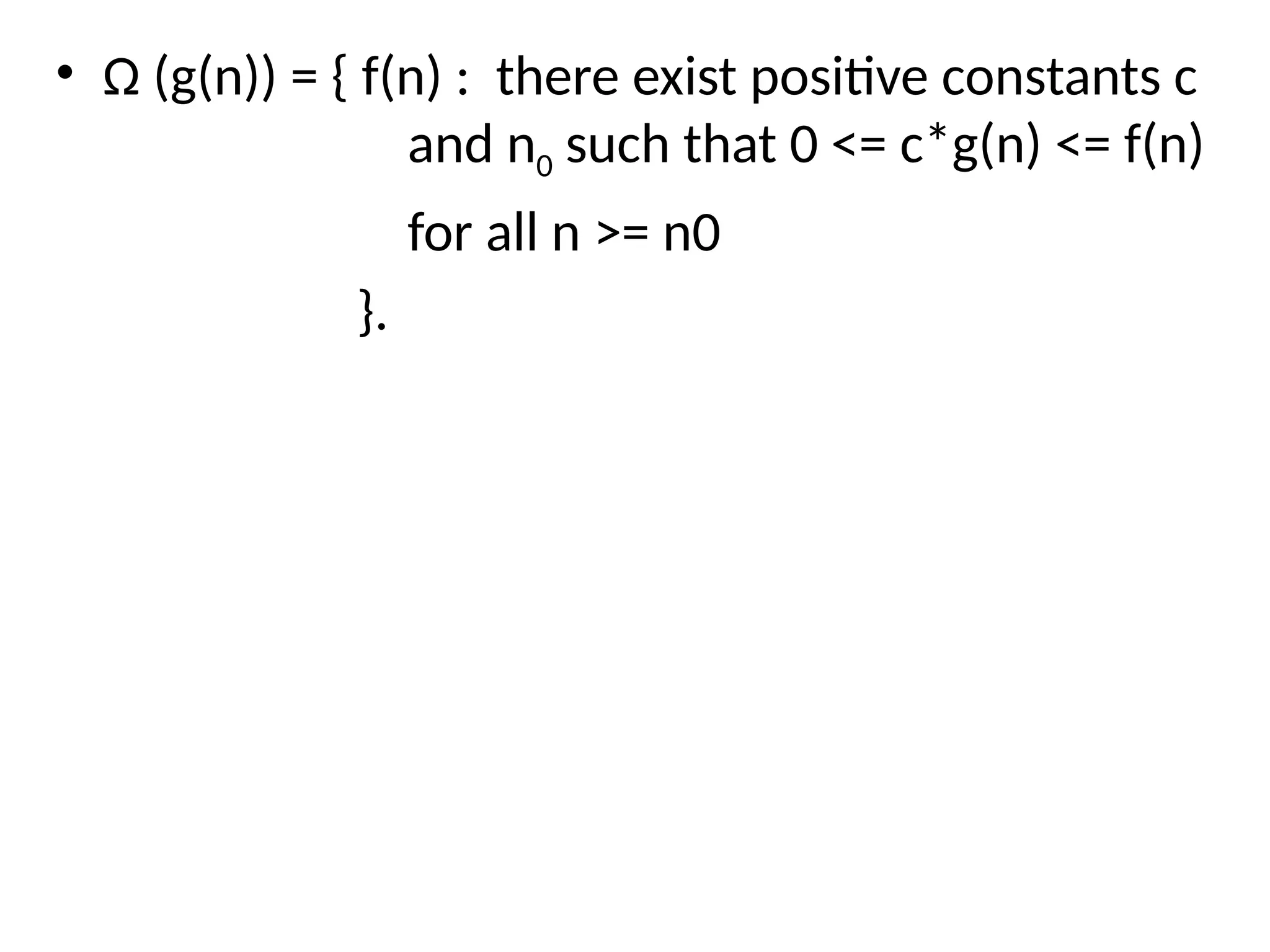
• Ω Notation:Just as Big O notation provides an asymptotic upper bound on a function, Ω notation provides an asymptotic lower bound. • Ω Notation : can be useful when we have lower bound on time complexity of an algorithm. • The best case performance of an algorithm is generall y not useful , the Omega notation is the least used notation among all three. • For a given function g(n), we denote by Ω(g(n)) the set of functions.
51.
• Ω (g(n))= { f(n) : there exist positive constants c and n0 such that 0 <= c*g(n) <= f(n) for all n >= n0 }.
52.
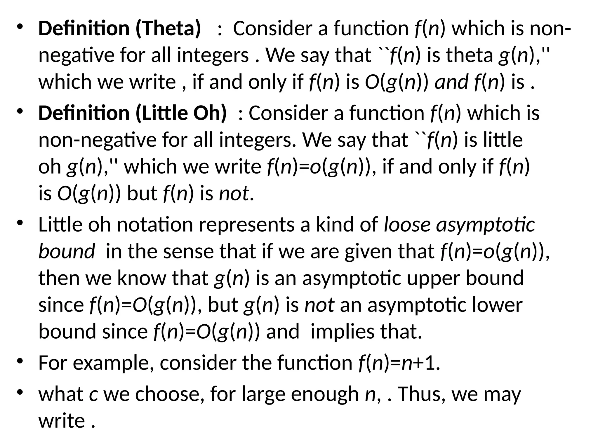
• Definition (Theta): Consider a function f(n) which is non- negative for all integers . We say that ``f(n) is theta g(n),'' which we write , if and only if f(n) is O(g(n)) and f(n) is . • Definition (Little Oh) : Consider a function f(n) which is non-negative for all integers. We say that ``f(n) is little oh g(n),'' which we write f(n)=o(g(n)), if and only if f(n) is O(g(n)) but f(n) is not. • Little oh notation represents a kind of loose asymptotic bound in the sense that if we are given that f(n)=o(g(n)), then we know that g(n) is an asymptotic upper bound since f(n)=O(g(n)), but g(n) is not an asymptotic lower bound since f(n)=O(g(n)) and implies that. • For example, consider the function f(n)=n+1. • what c we choose, for large enough n, . Thus, we may write .
53.
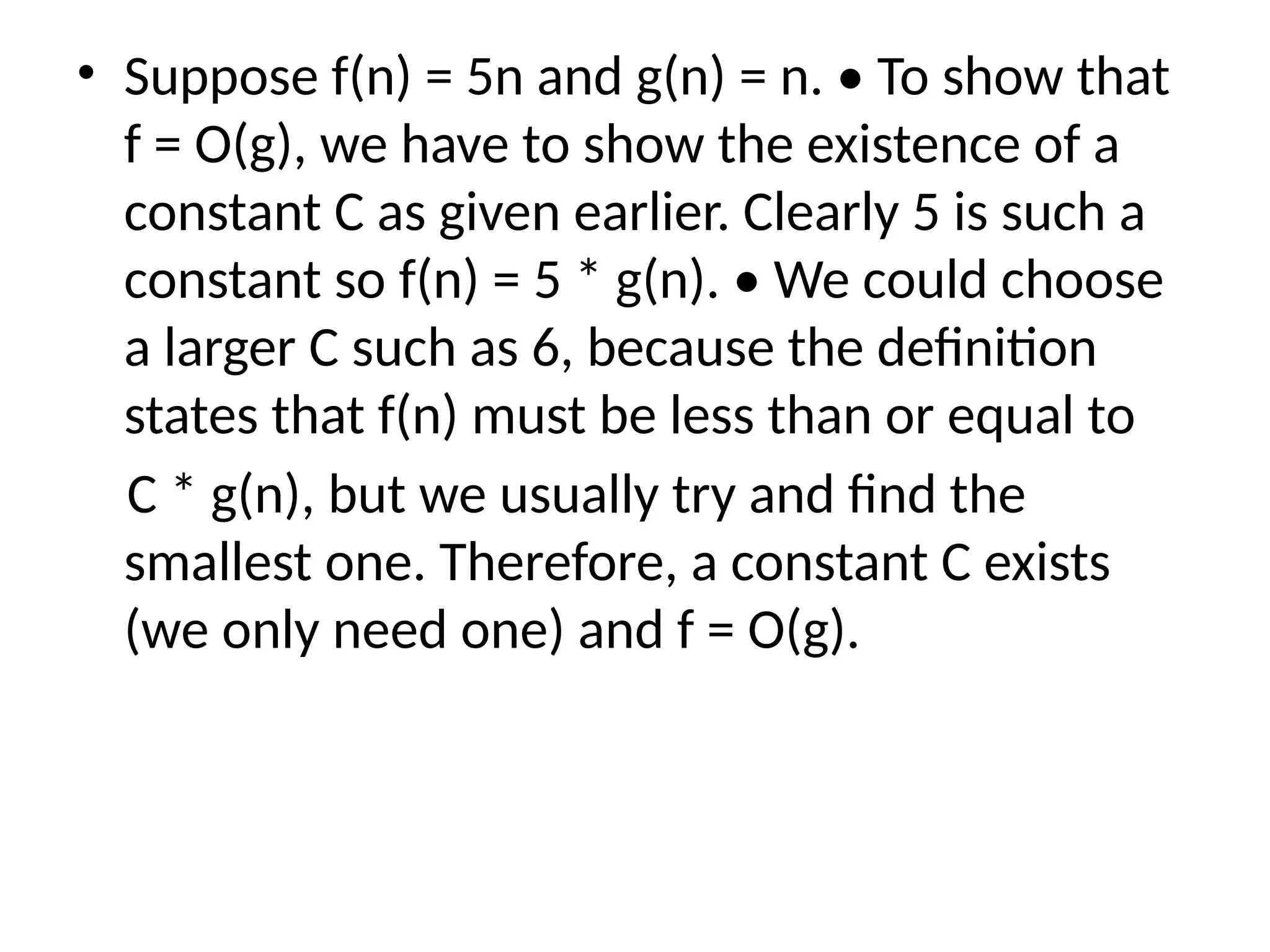
• Suppose f(n)= 5n and g(n) = n. • To show that f = O(g), we have to show the existence of a constant C as given earlier. Clearly 5 is such a constant so f(n) = 5 * g(n). • We could choose a larger C such as 6, because the definition states that f(n) must be less than or equal to C * g(n), but we usually try and find the smallest one. Therefore, a constant C exists (we only need one) and f = O(g).
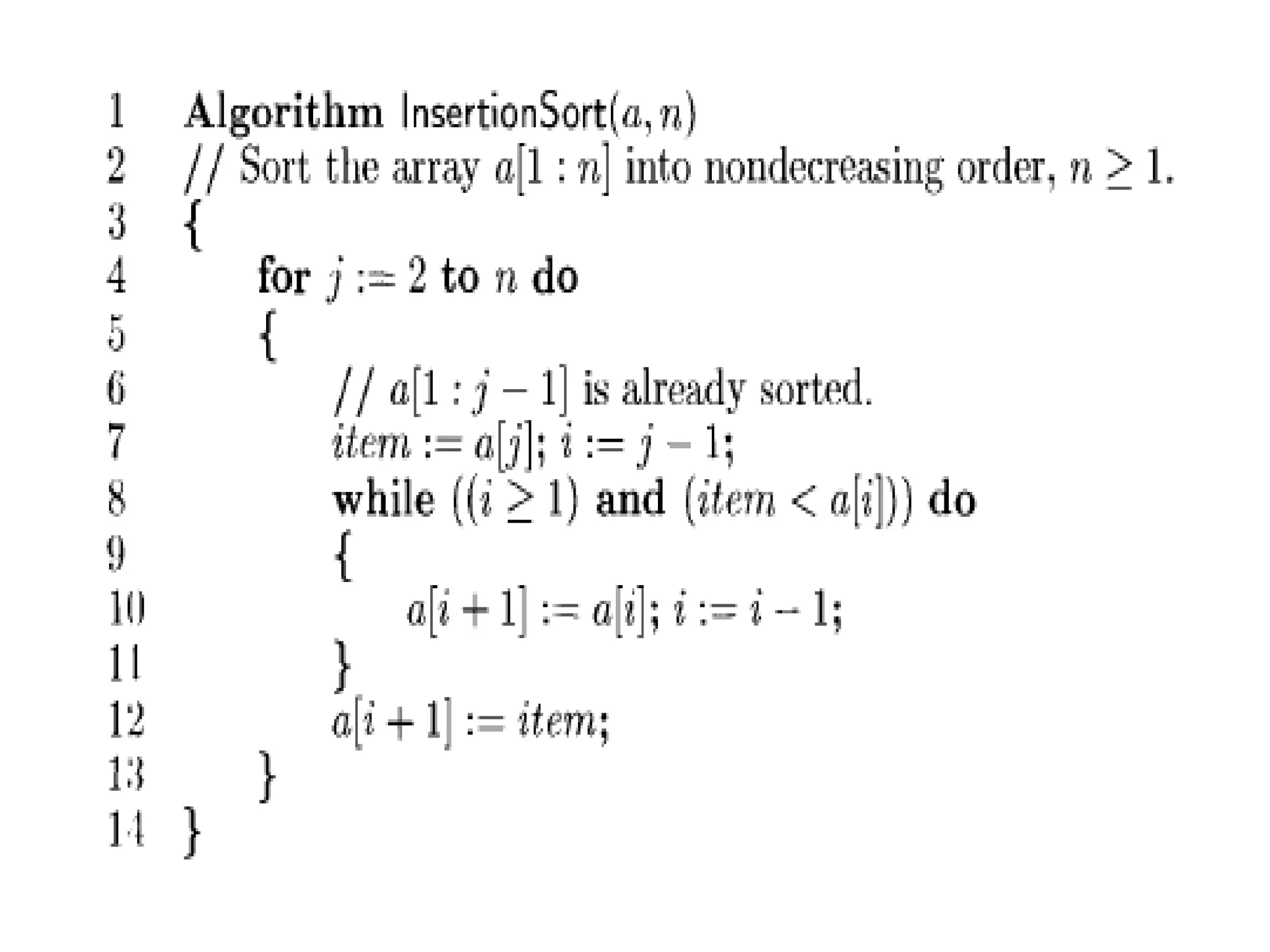
Time Complexity ofinsertion sort : If we take a closer look at the insertion sort code, we can notice that every iteration of while loop reduces one inversion. The while loop executes only if i > j and arr[i] < arr[j]. Therefore total number of while loop iterations (For all values of i) is same as number of inversions. Therefore overall time complexity of the insertion sort is O(n + f(n)) where f(n) is inversion count. If the inversion count is O(n), then the time complexity of insertion sort is O(n). In worst case, there can be n*(n-1)/2 inversions. The worst case occurs when the array is sorted in reverse order. So the worst case time complexity of insertion sort is O(n2 ).
![#include<stdio . h> int main() { int n, i, sum=0; scanf(“%d”, &n); int arr[n]; for(I = 0; i<n; i++) { scanf(“%d”, & arr[i]); sum= sum + arr[i];} printf(“%d”, sum); }](https://image.slidesharecdn.com/chapter1daa-250929095022-94a9c7e9/75/Design-and-analysis-of-algorithms-introduction-to-algorithms-pptx-24-2048.jpg)
![int sum (int a[], int n) { int x =0; For (int i=0; i<n ; i++) { x = x+ a[i]; } return (x); }](https://image.slidesharecdn.com/chapter1daa-250929095022-94a9c7e9/75/Design-and-analysis-of-algorithms-introduction-to-algorithms-pptx-26-2048.jpg)
![1. Algorithm Sum(a[ ], n) 2. { 3. s:= 0.0; 4. for i = 1 to n do 5. s := s + a[i]; 6. return s; 7. }](https://image.slidesharecdn.com/chapter1daa-250929095022-94a9c7e9/75/Design-and-analysis-of-algorithms-introduction-to-algorithms-pptx-29-2048.jpg)
![• Every instance needs to store array a[] & n. – Space needed to store n = 1 word. – Space needed to store a[ ] = n floating point words (or at least n words) – Space needed to store i and s = 2 words • Sp(n) = (n + 3). Hence S(P) = (n + 3).](https://image.slidesharecdn.com/chapter1daa-250929095022-94a9c7e9/75/Design-and-analysis-of-algorithms-introduction-to-algorithms-pptx-30-2048.jpg)
![Statements S/E Freq. Total 1 Algorithm Sum(a[ ],n) 0 - 0 2 { 0 - 0 3 S = 0.0; 1 1 1 4 for i=1 to n do 1 n+1 n+1 5 s = s+a[i]; 1 n n 6 return s; 1 1 1 7 } 0 - 0 2n+3](https://image.slidesharecdn.com/chapter1daa-250929095022-94a9c7e9/75/Design-and-analysis-of-algorithms-introduction-to-algorithms-pptx-37-2048.jpg)
![Statements S/E Freq. Total 1 Algorithm Sum(a[ ],n,m) 0 - 0 2 { 0 - 0 3 for i=1 to n do; 1 n+1 n+1 4 for j=1 to m do 1 n(m+1) n(m+1) 5 s = s+a[i][j]; 1 nm nm 6 return s; 1 1 1 7 } 0 - 0 2nm+2n+2](https://image.slidesharecdn.com/chapter1daa-250929095022-94a9c7e9/75/Design-and-analysis-of-algorithms-introduction-to-algorithms-pptx-38-2048.jpg)
![int sum(int a[], int n) { int r = 0; for (int i = 0; i < n; ++i) { r += a[i]; } return r; } requires N units for a, plus space for n, r and i, so it's O(N).](https://image.slidesharecdn.com/chapter1daa-250929095022-94a9c7e9/75/Design-and-analysis-of-algorithms-introduction-to-algorithms-pptx-43-2048.jpg)
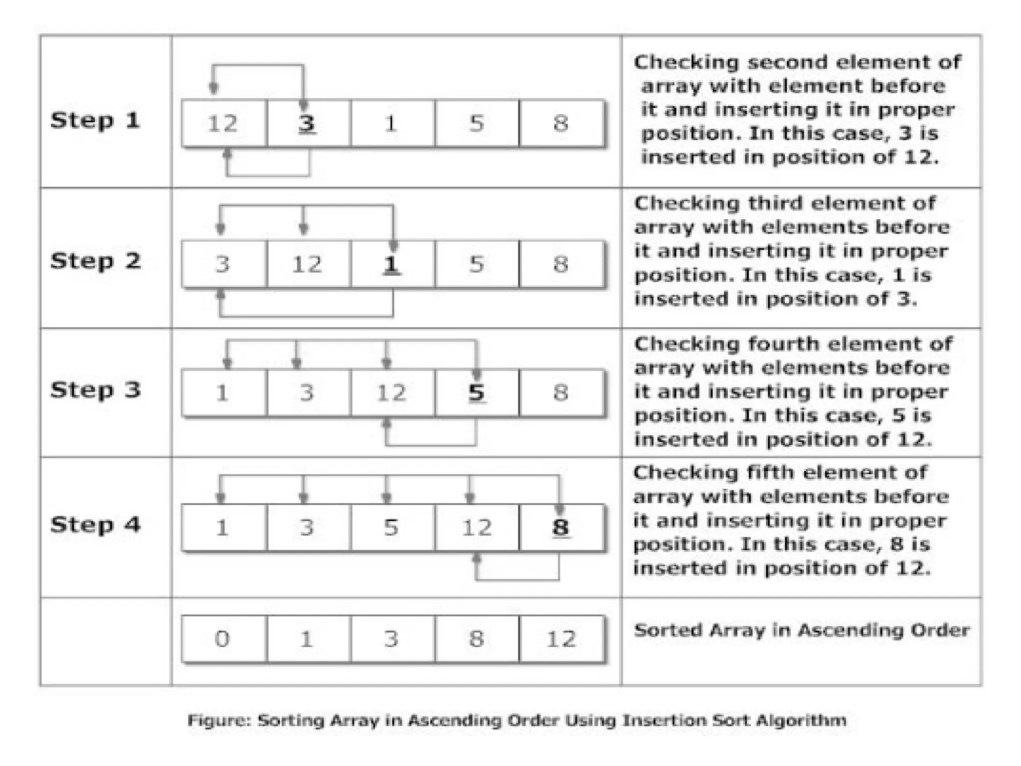
![Insertion Sort for(i=1; i<n ; i++) { temp = data[i]; j=i-1; while(temp<data[j] && j>=0) {data[j+1] = data[j]; --j; } data[j+1]=temp; } printf("In ascending order: "); for(i=0; i<n; i++) printf("%dt",data[i]); return 0; }](https://image.slidesharecdn.com/chapter1daa-250929095022-94a9c7e9/75/Design-and-analysis-of-algorithms-introduction-to-algorithms-pptx-55-2048.jpg)
![Time Complexity of insertion sort : If we take a closer look at the insertion sort code, we can notice that every iteration of while loop reduces one inversion. The while loop executes only if i > j and arr[i] < arr[j]. Therefore total number of while loop iterations (For all values of i) is same as number of inversions. Therefore overall time complexity of the insertion sort is O(n + f(n)) where f(n) is inversion count. If the inversion count is O(n), then the time complexity of insertion sort is O(n). In worst case, there can be n*(n-1)/2 inversions. The worst case occurs when the array is sorted in reverse order. So the worst case time complexity of insertion sort is O(n2 ).](https://image.slidesharecdn.com/chapter1daa-250929095022-94a9c7e9/75/Design-and-analysis-of-algorithms-introduction-to-algorithms-pptx-57-2048.jpg)