Downloaded 16 times
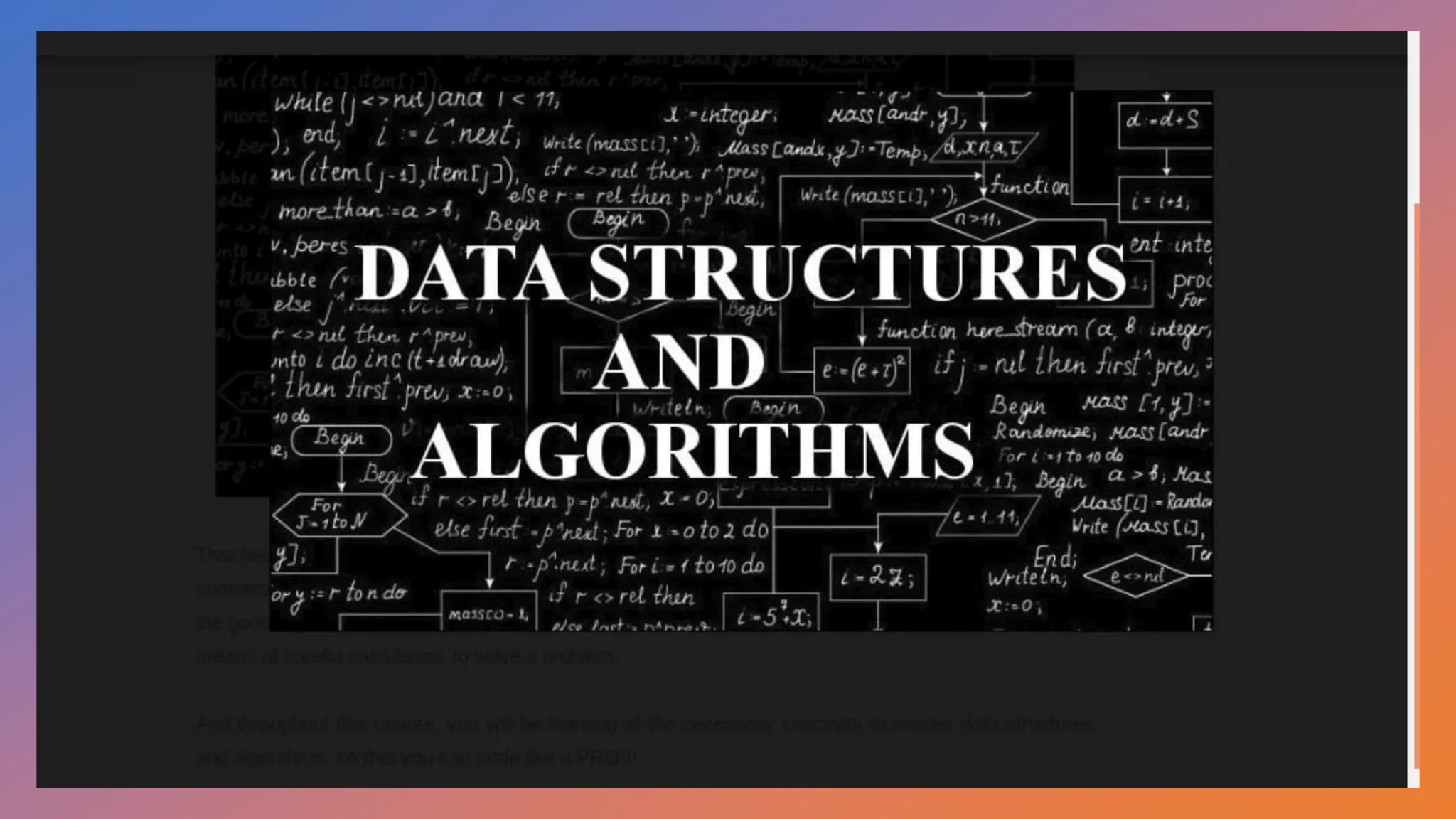


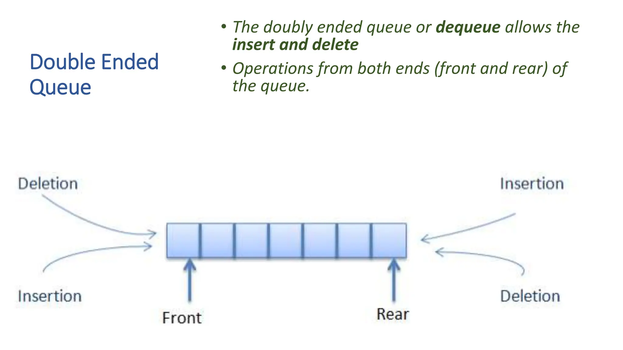


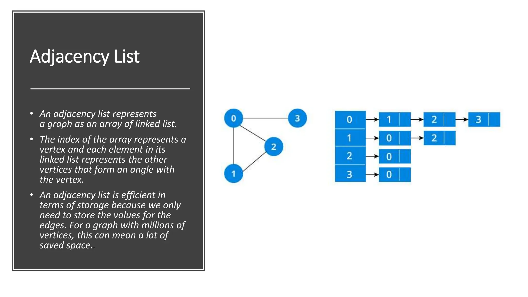
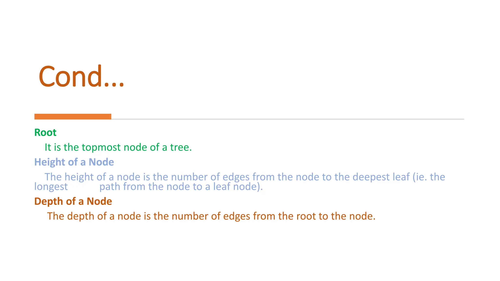
![Adjacency Matrix • An adjacency matrix is 2D array of V x V vertices. Each row and column represent a vertex. • If the value of any element a[i][j] is 1, it represents that there is an edge connecting vertex i and vertex j . • Since it is an undirected graph, for edge (0,2), we also need to mark edge (2,0); making the adjacency matrix symmetric about the diagonal. • Edge lookup(checking if an edge exists between vertex A and vertex B) is extremely fast in adjacency matrix representation but we have to reserve space for every possible link between all vertices(V x V), so it requires more space.](https://image.slidesharecdn.com/datastructuresandalgorithms-240504174600-0f0445b8/75/Data-Structures-and-Algorithms-Fundamentals-49-2048.jpg)
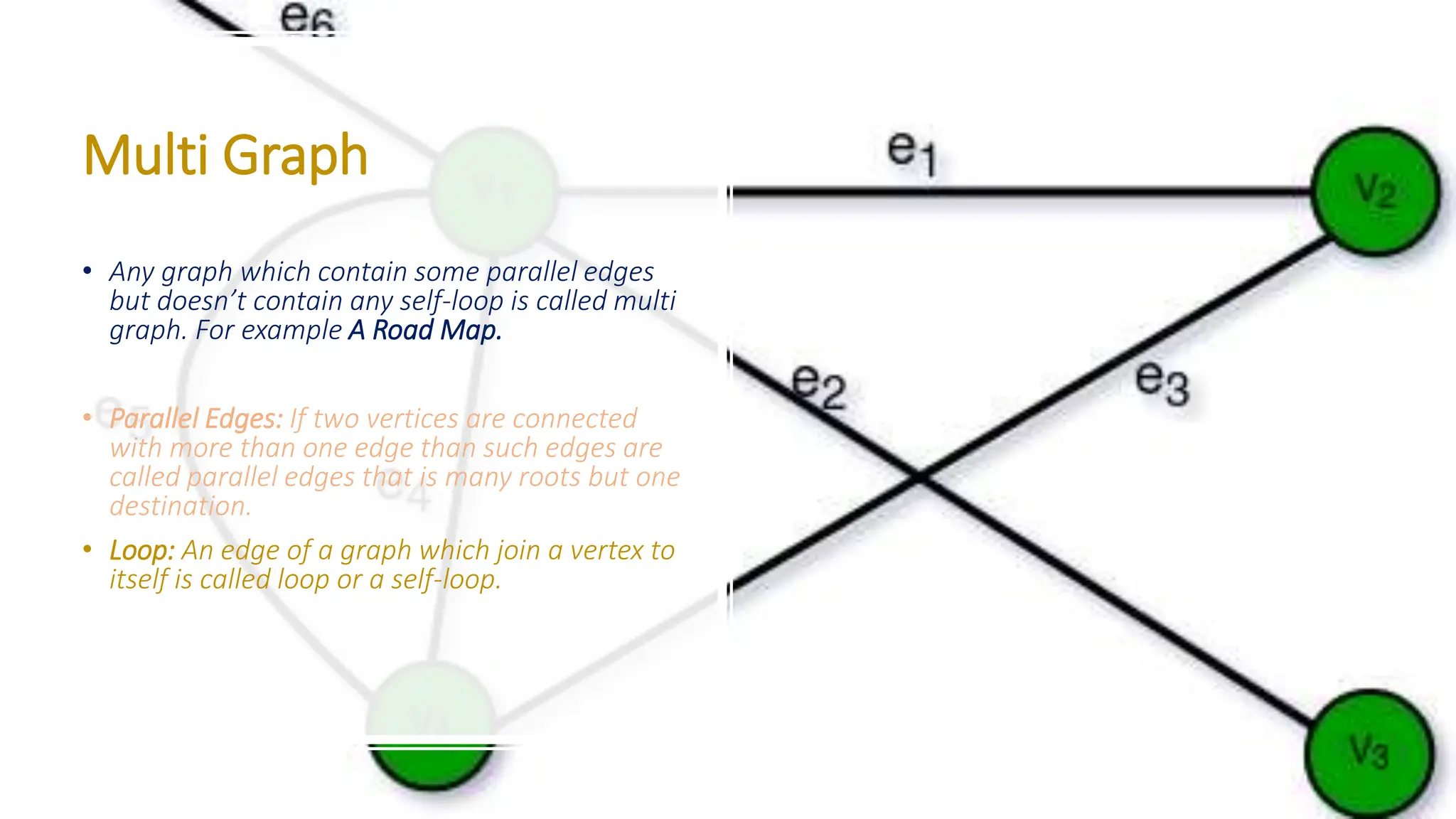
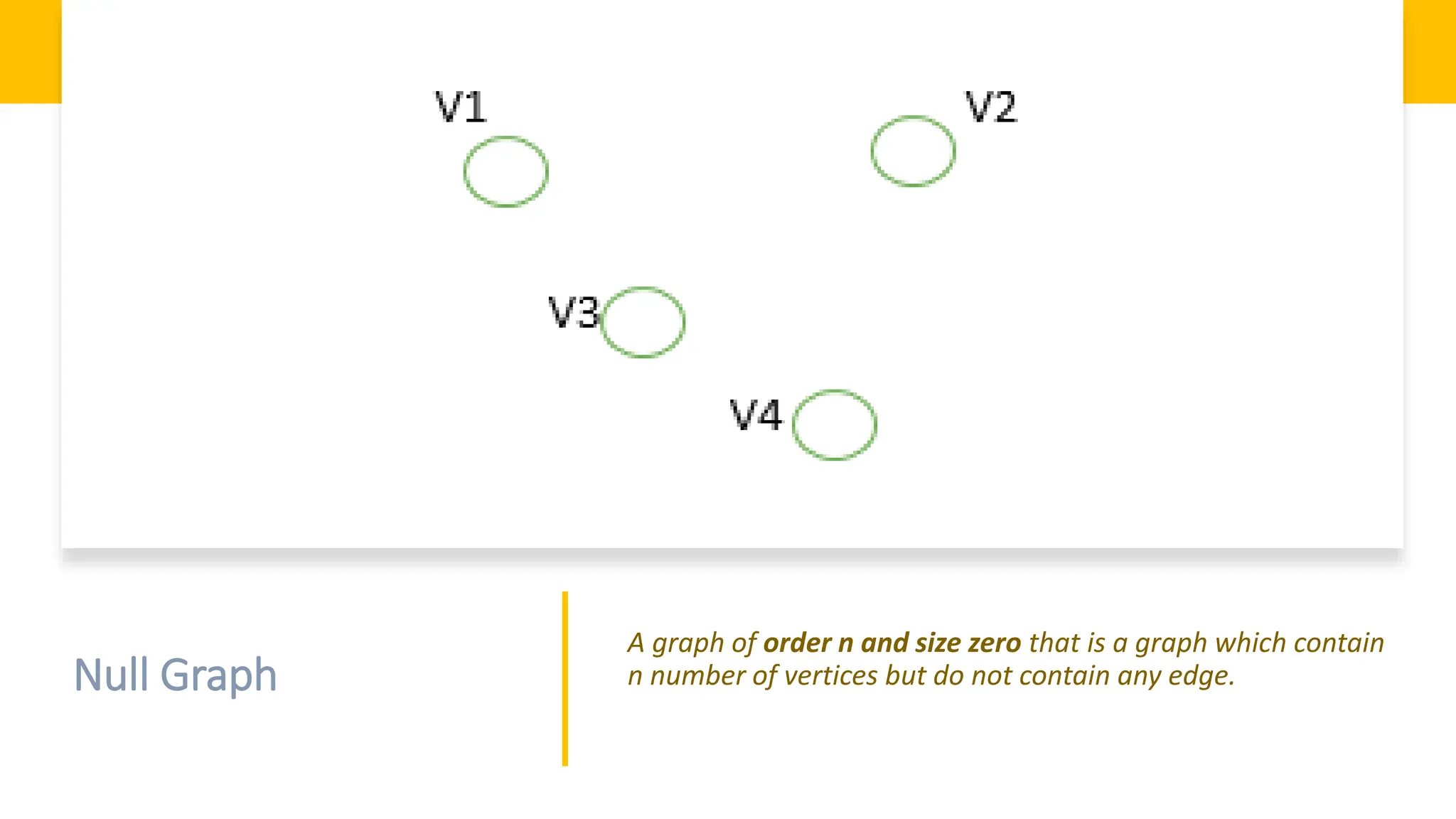
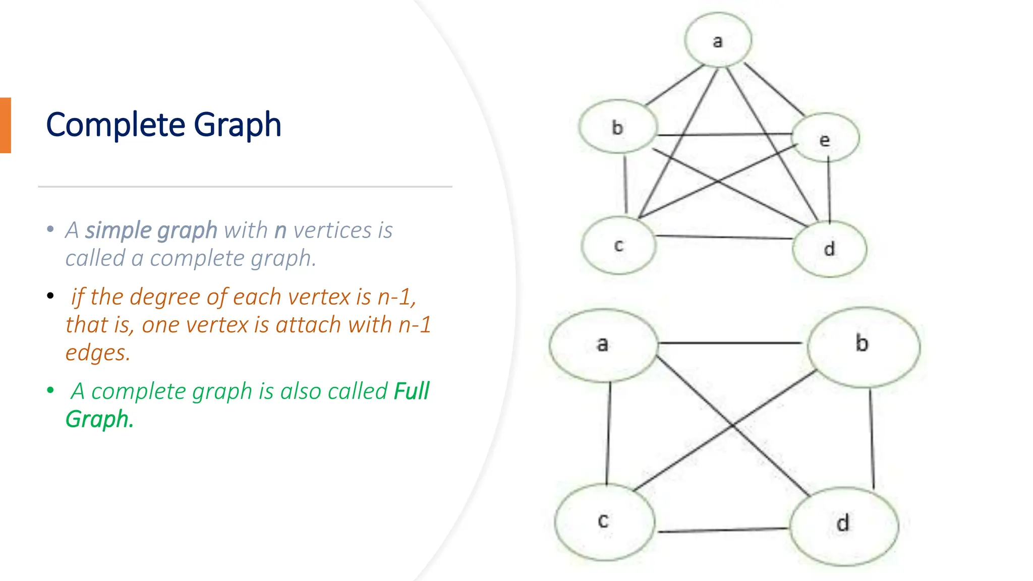
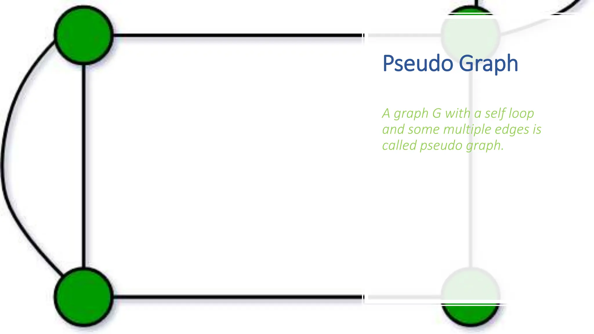
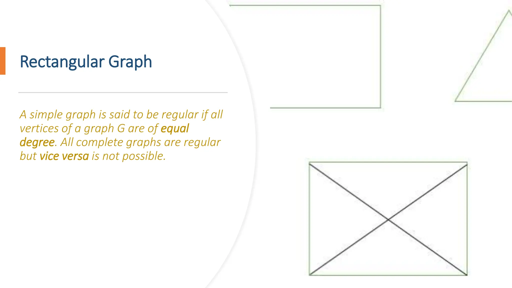
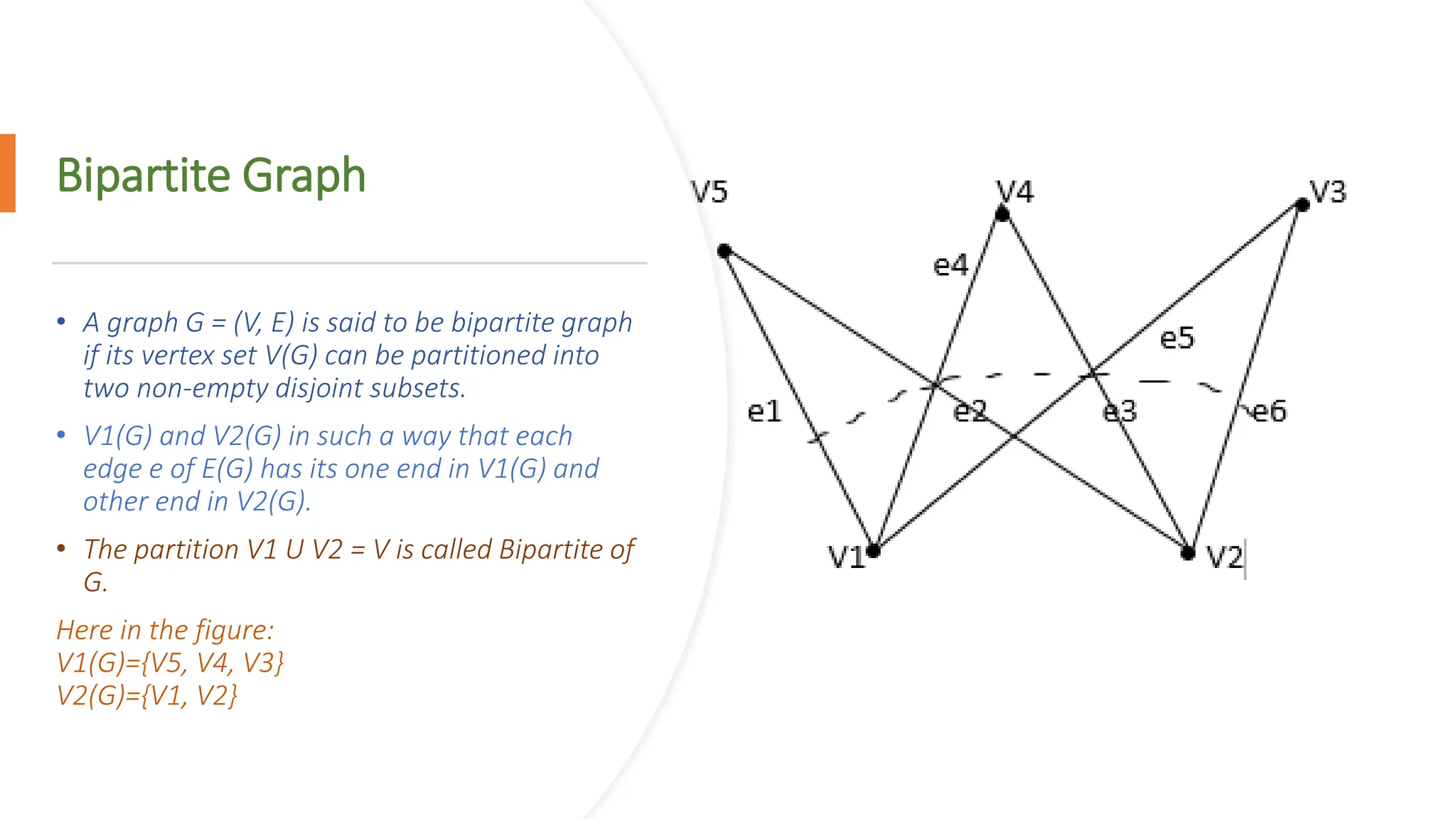
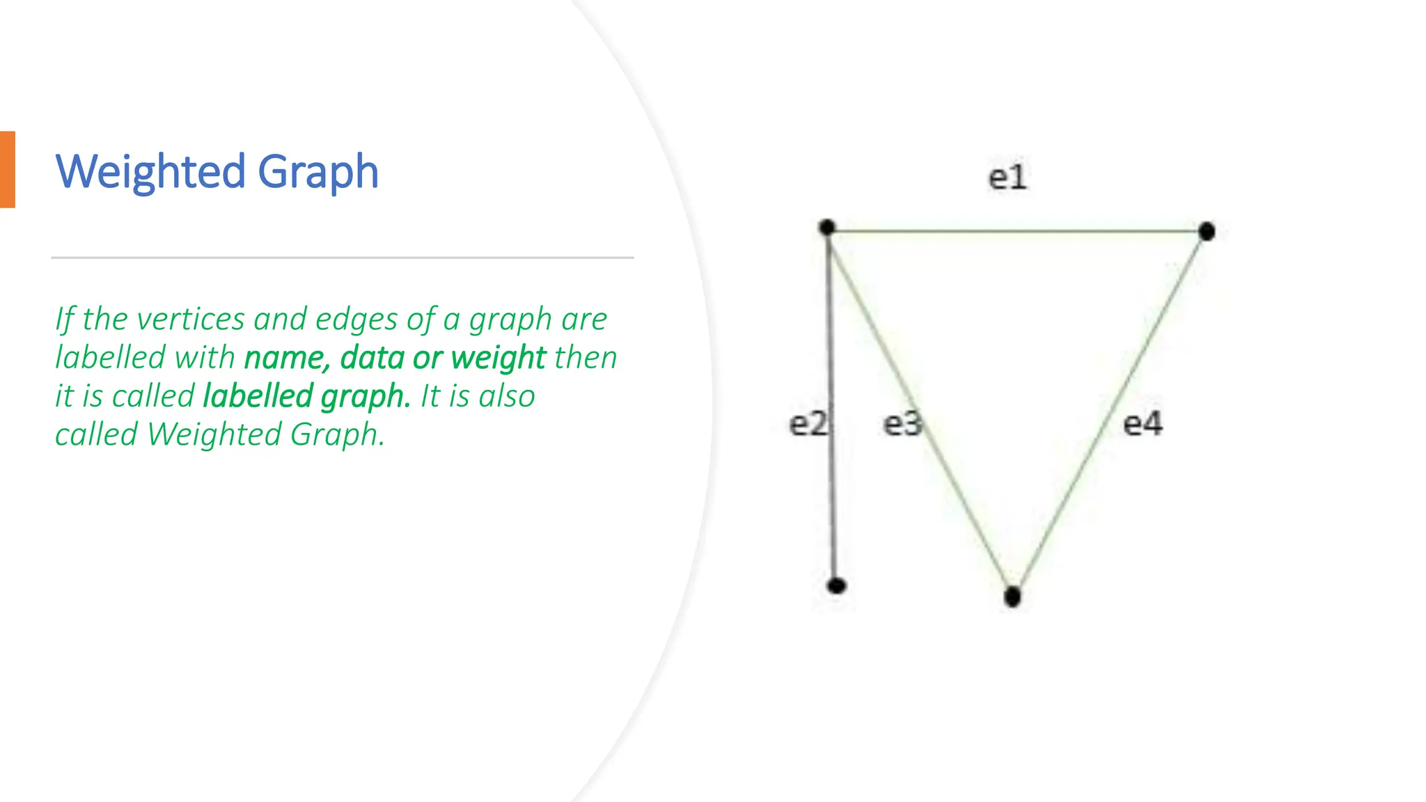
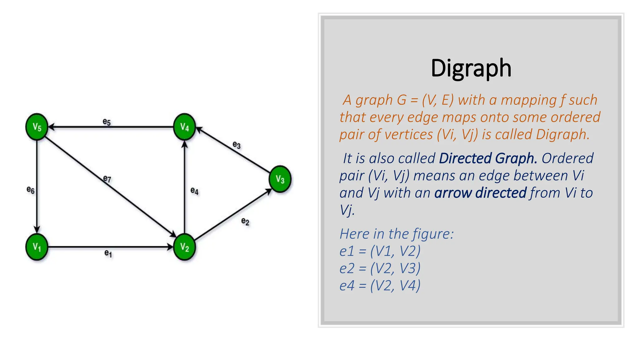
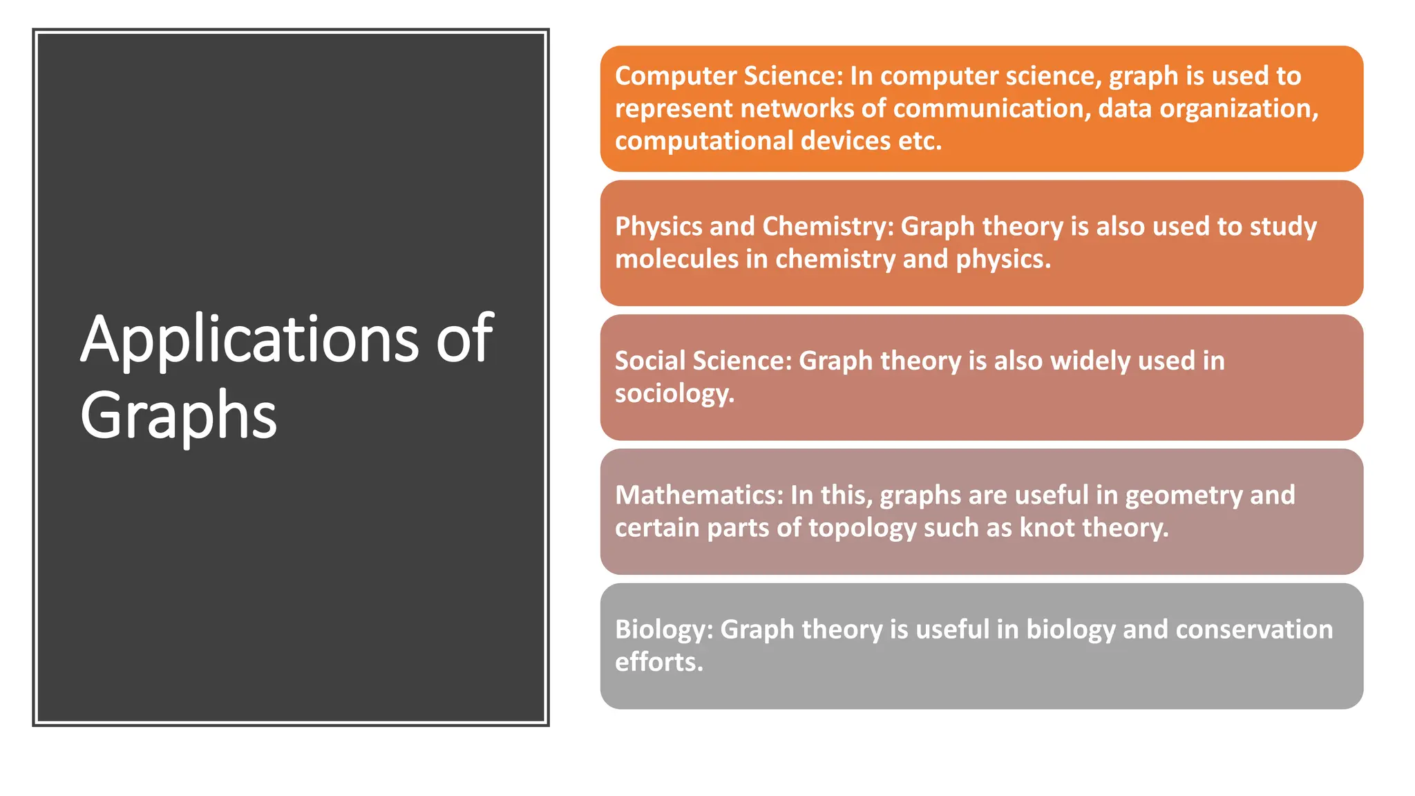

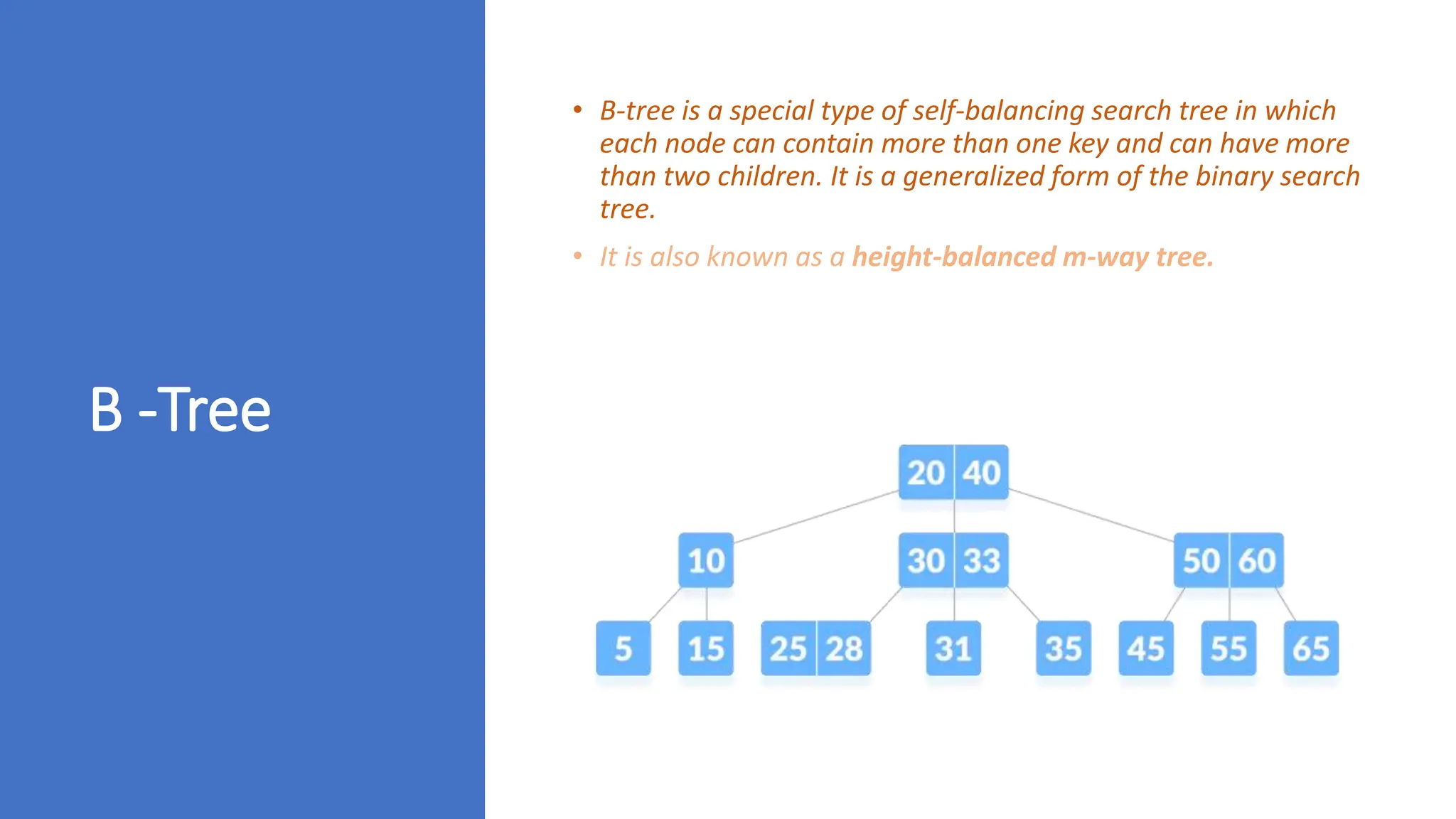
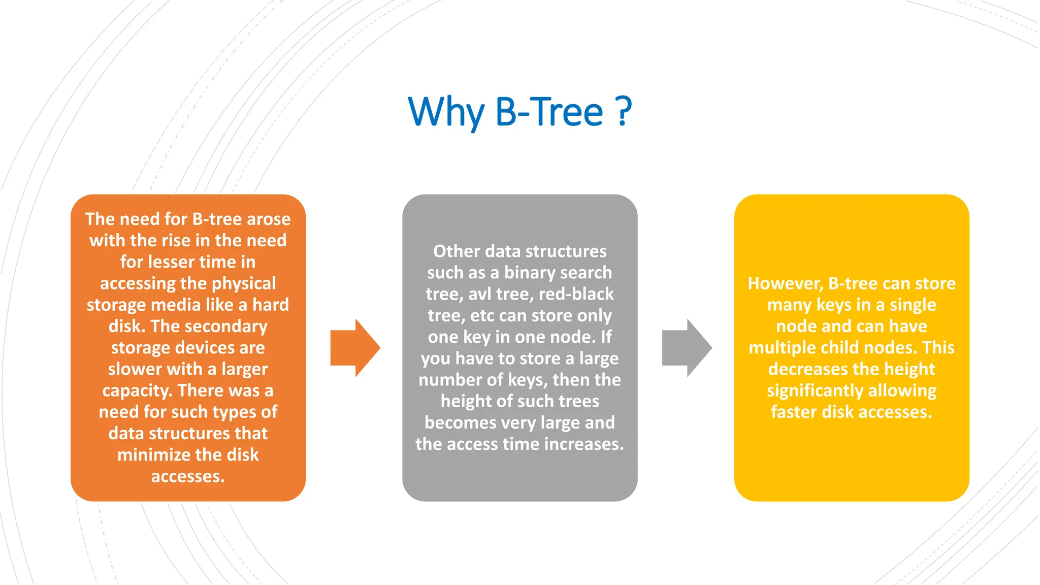
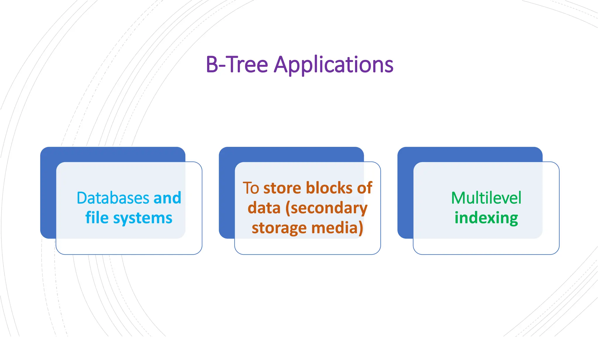


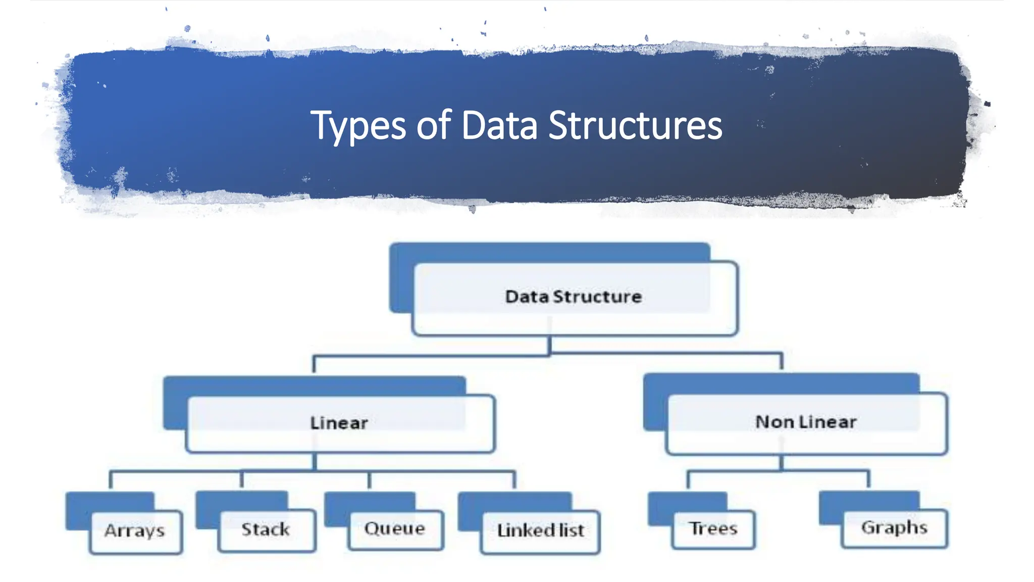
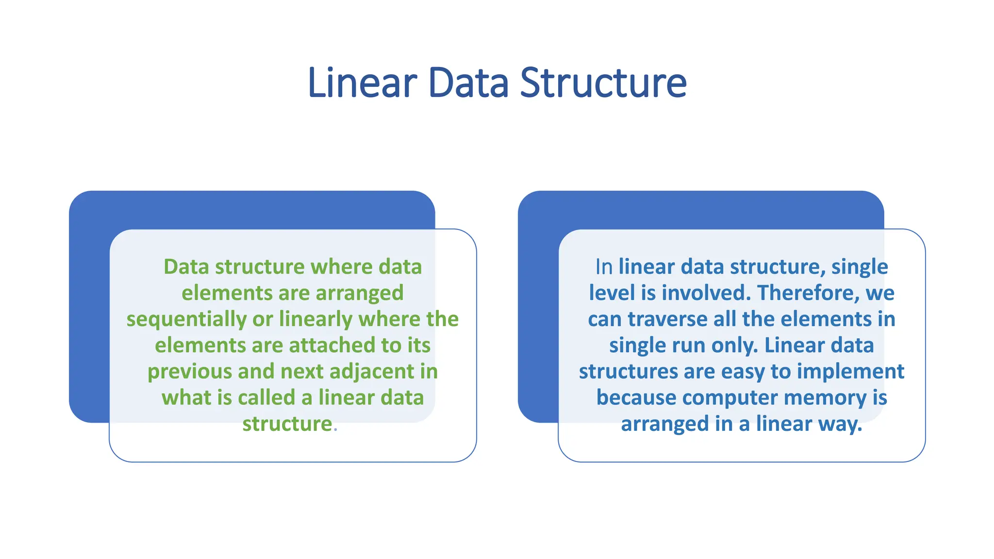
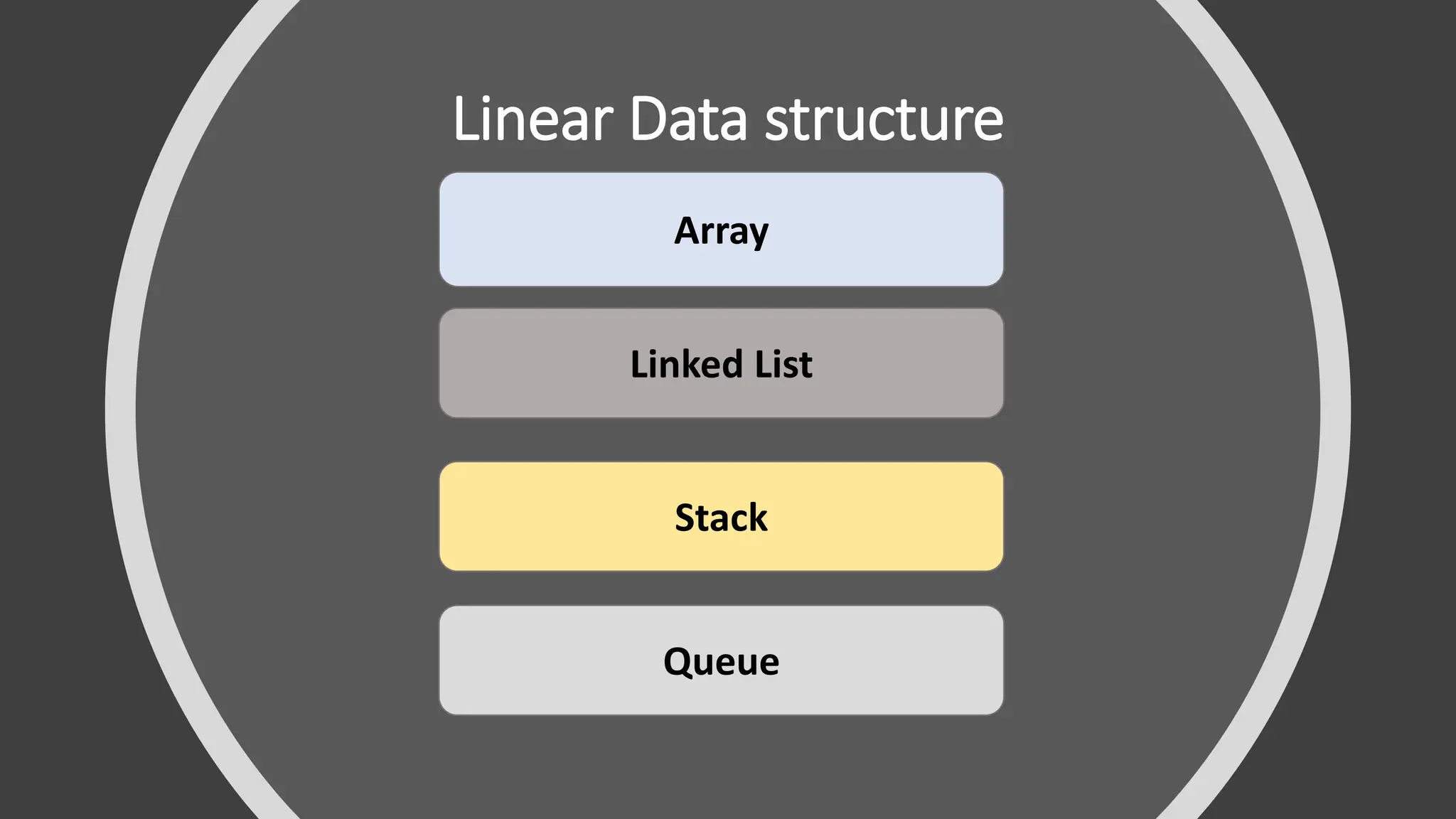
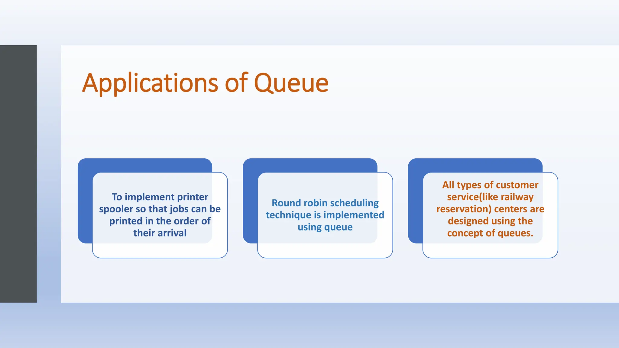
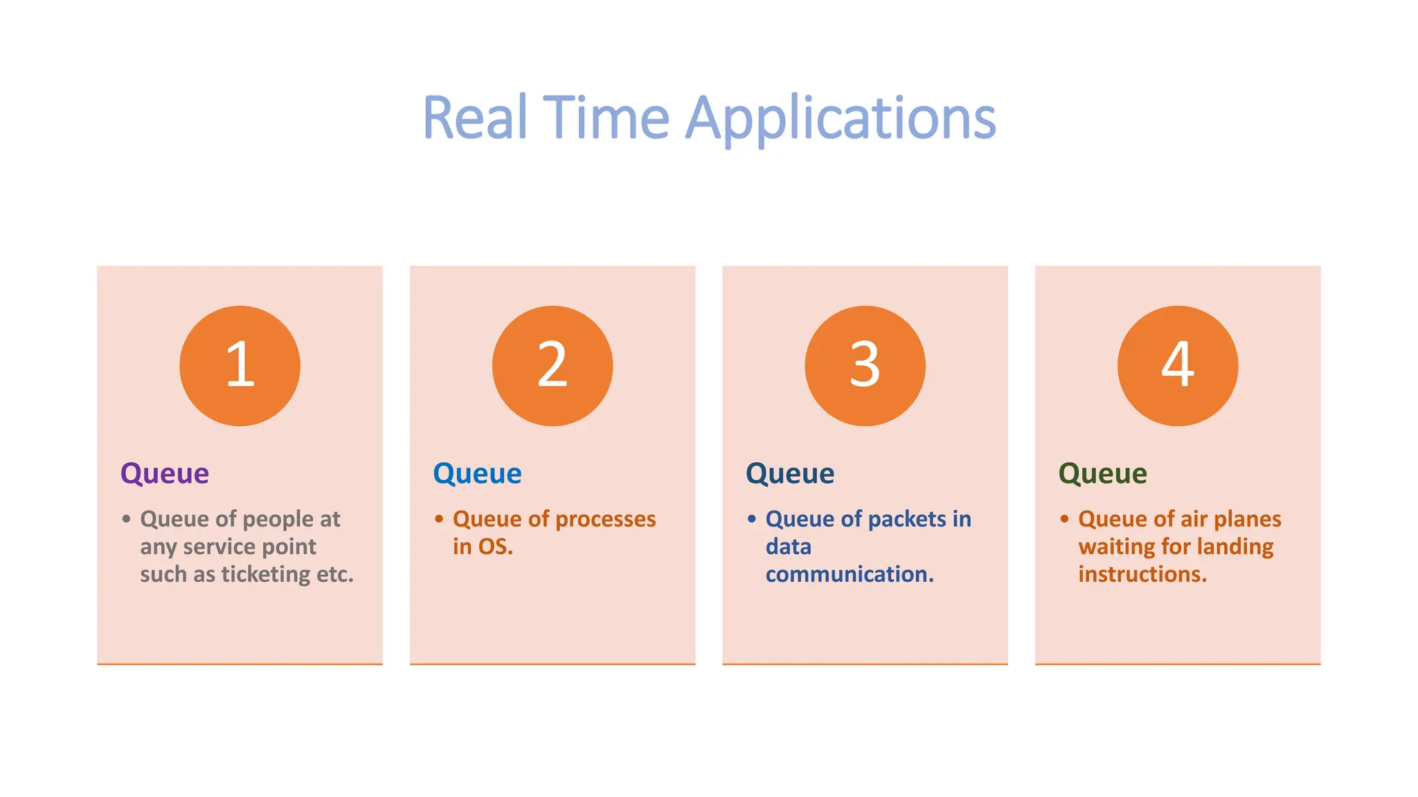
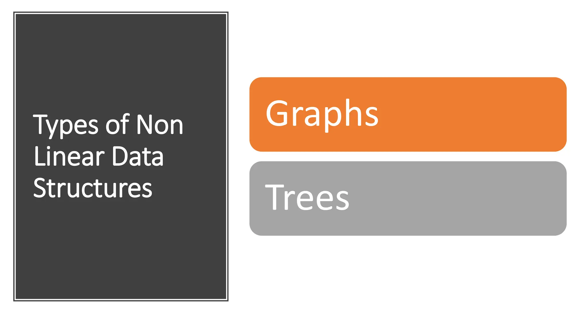
The document provides a comprehensive overview of data structures in computer science, detailing programming concepts and the classification of data structures into linear and non-linear types. It covers various linear data structures such as arrays, stacks, and queues, as well as non-linear structures like graphs and trees, including their properties, operations, and real-time applications. Additionally, it highlights the importance of efficient data organization for performance in programming and computational tasks.