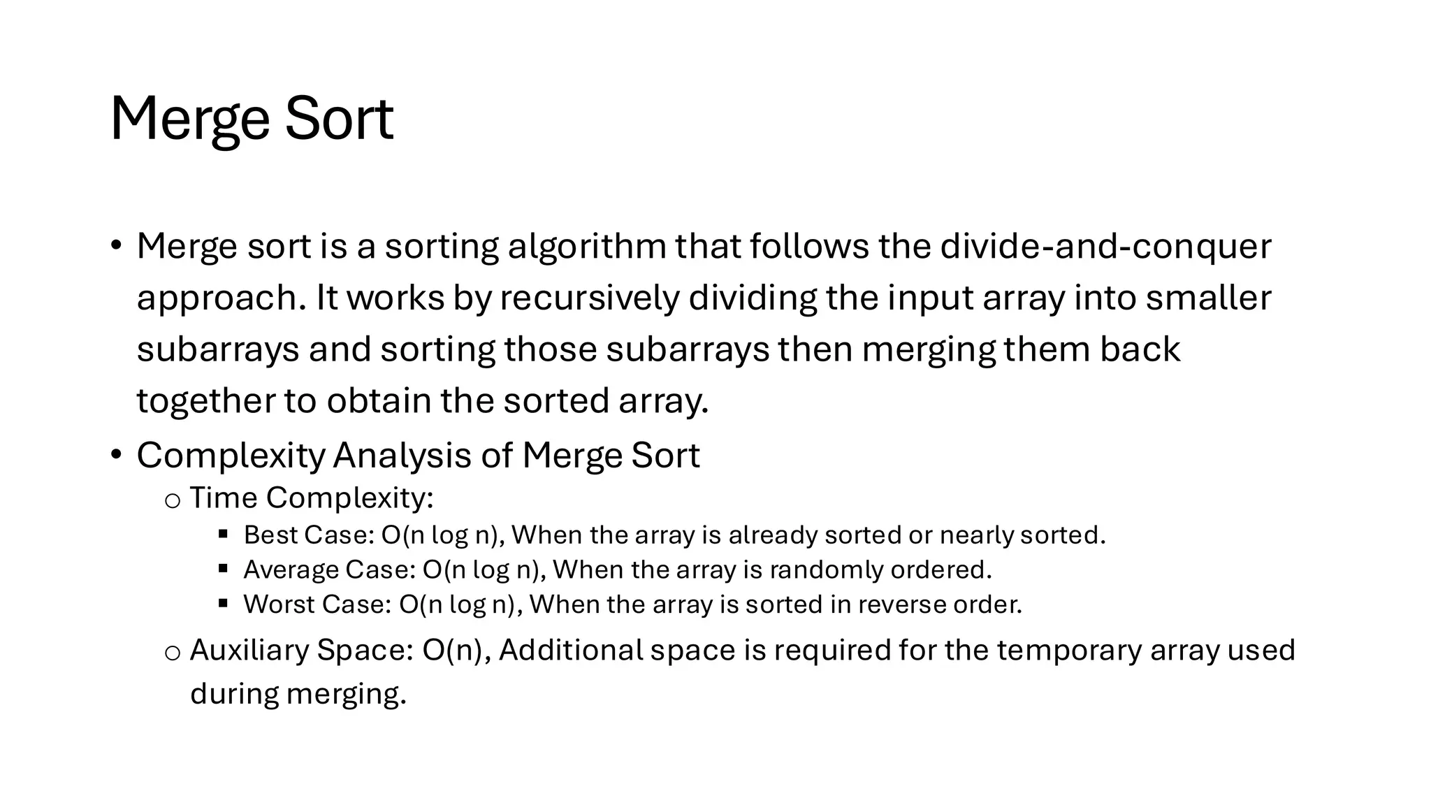
Download as PDF, PPTX
![Types of Array • Static Array: A collection of elements stored in contiguous memory locations. • int arr[5] = {1, 2, 3, 4, 5}; • Dynamic Array: A Dynamic Array is an array that can grow or shrink in size automatically during runtime. • int* arr = new int[5]; • delete[] arr;](https://image.slidesharecdn.com/datastructuresalgorithms-spring2025-250407112227-d7e7a1f6/75/Data-Structures-Algorithms-Spring-2025-pdf-9-2048.jpg)
![Dynamic Array vs. Static Array Operation Static Array Dynamic Array Memory Location Stack Heap Resizable? NO Yes Efficiency Fast Slower Flexibility No Yes Access arr[i] O(1) O(1) Insertion at End Not Possible O(1) Insertion at Middle O(n) O(n) Delete at End Not Possible O(1) Delete at Middle O(n) O(n)](https://image.slidesharecdn.com/datastructuresalgorithms-spring2025-250407112227-d7e7a1f6/75/Data-Structures-Algorithms-Spring-2025-pdf-10-2048.jpg)
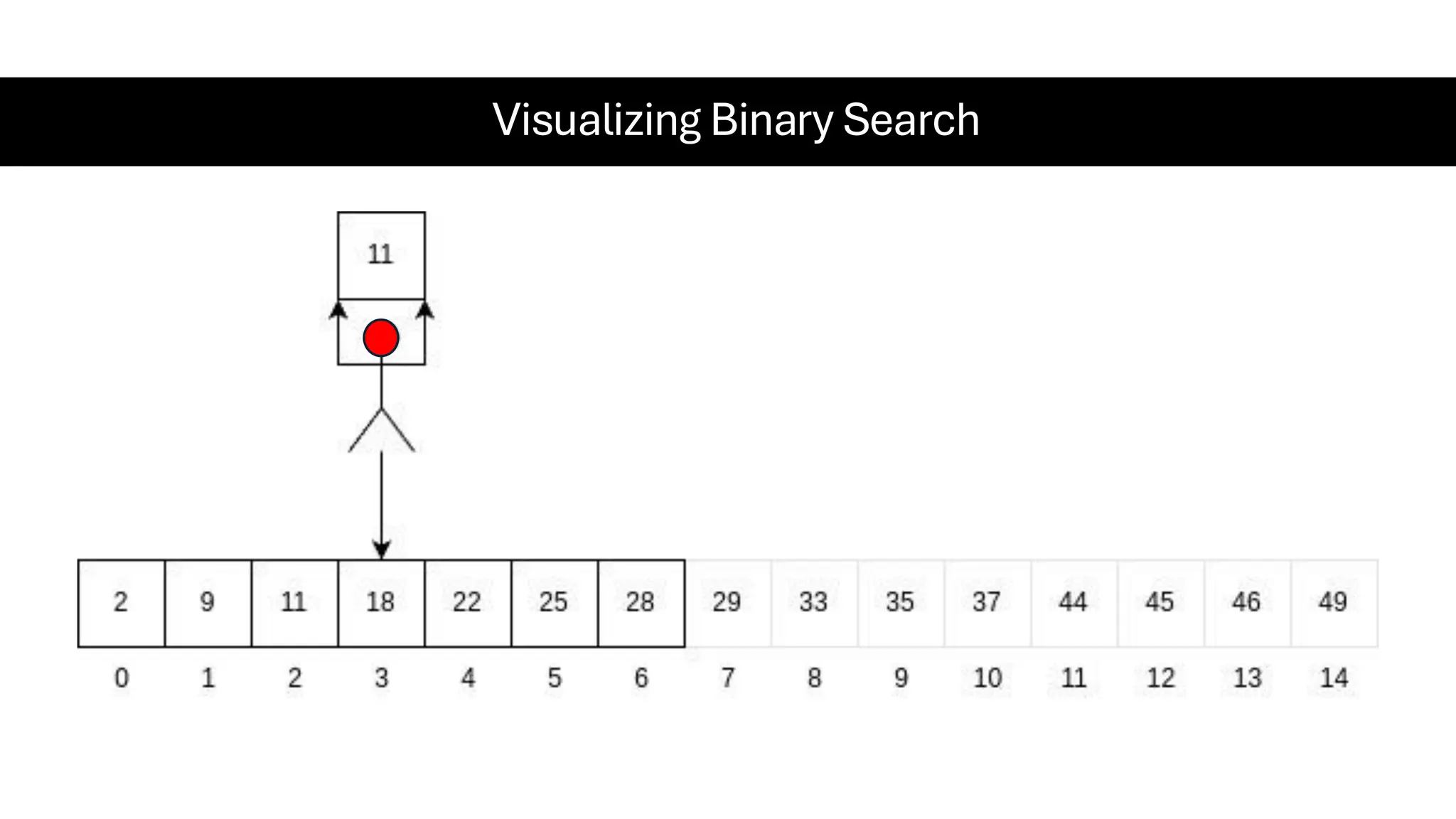
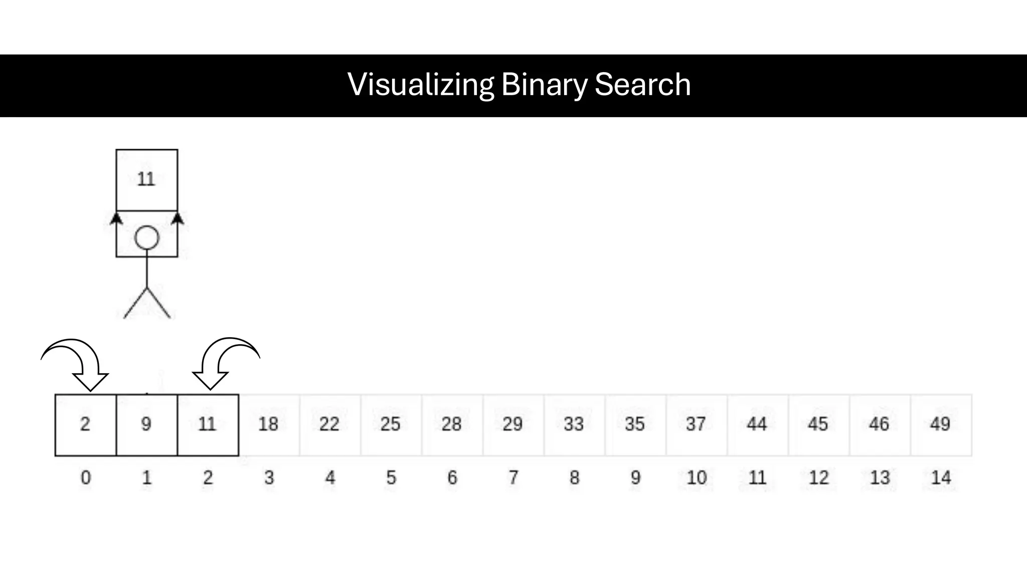
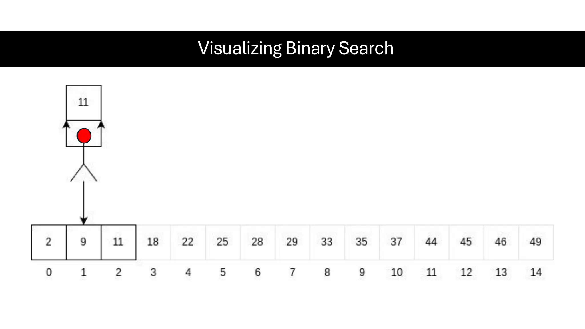
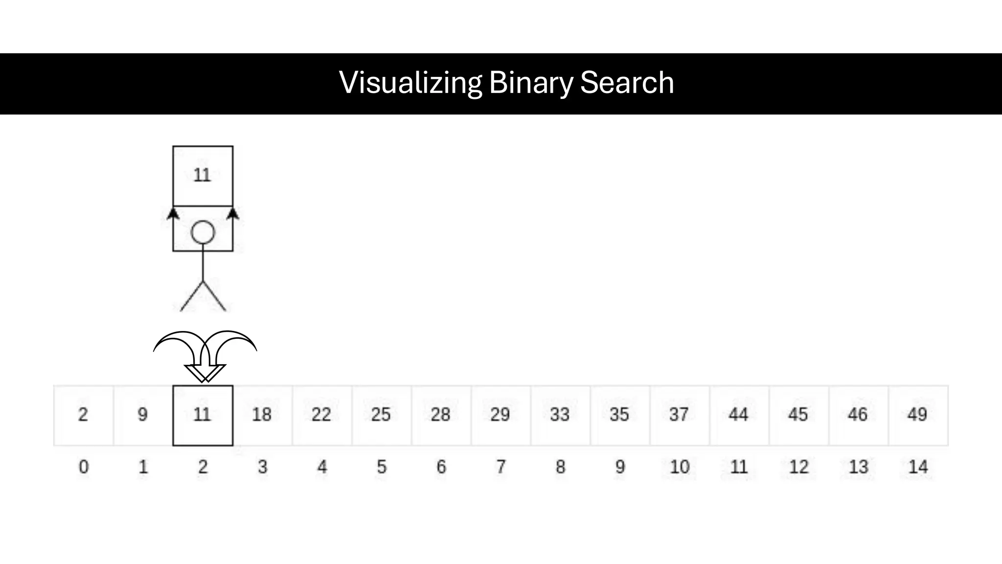
![Time Complexity Complexity Notation Example Constant Time O(1) Accessing an element in an array arr[i] Logarithmic Time O(log n) Binary Search Linear Time O(n) Iterating through an array Linearithmic Time O(n log n) Merge Sort, Quick Sort (average case) Quadratic Time O(n²) Nested loops (e.g., Bubble Sort) Cubic Time O(n³) Triple nested loops Exponential Time O(2ⁿ) Recursion in Fibonacci Factorial Time O(n!) Brute-force permutation generation](https://image.slidesharecdn.com/datastructuresalgorithms-spring2025-250407112227-d7e7a1f6/75/Data-Structures-Algorithms-Spring-2025-pdf-19-2048.jpg)


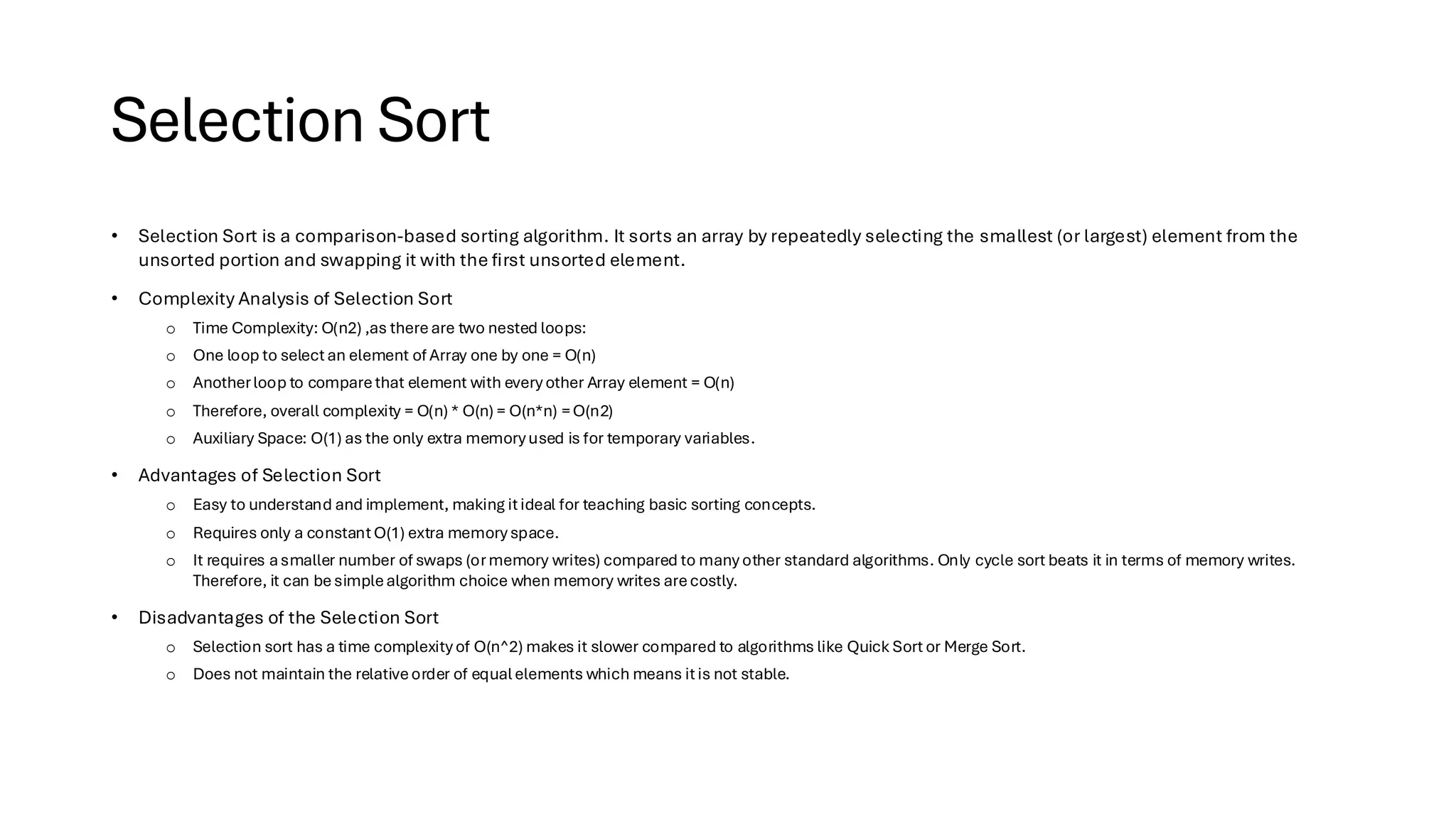


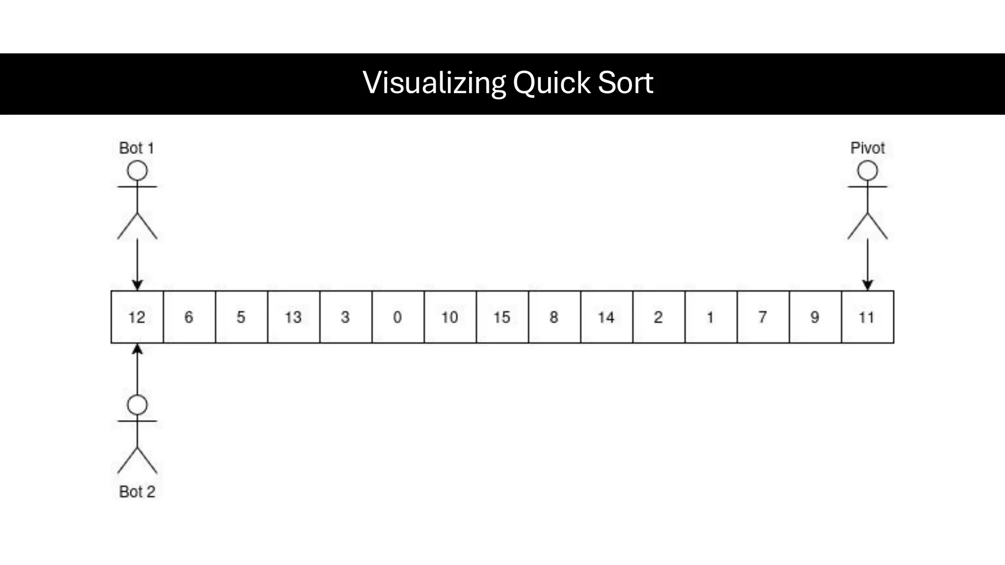


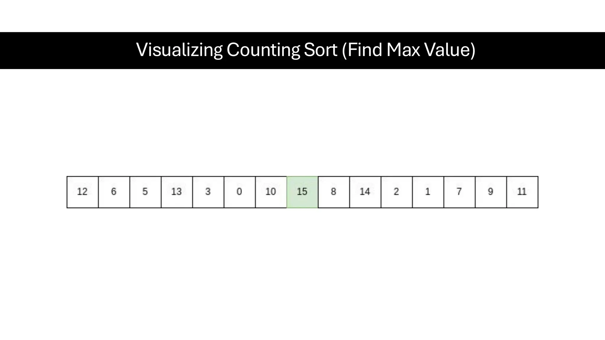
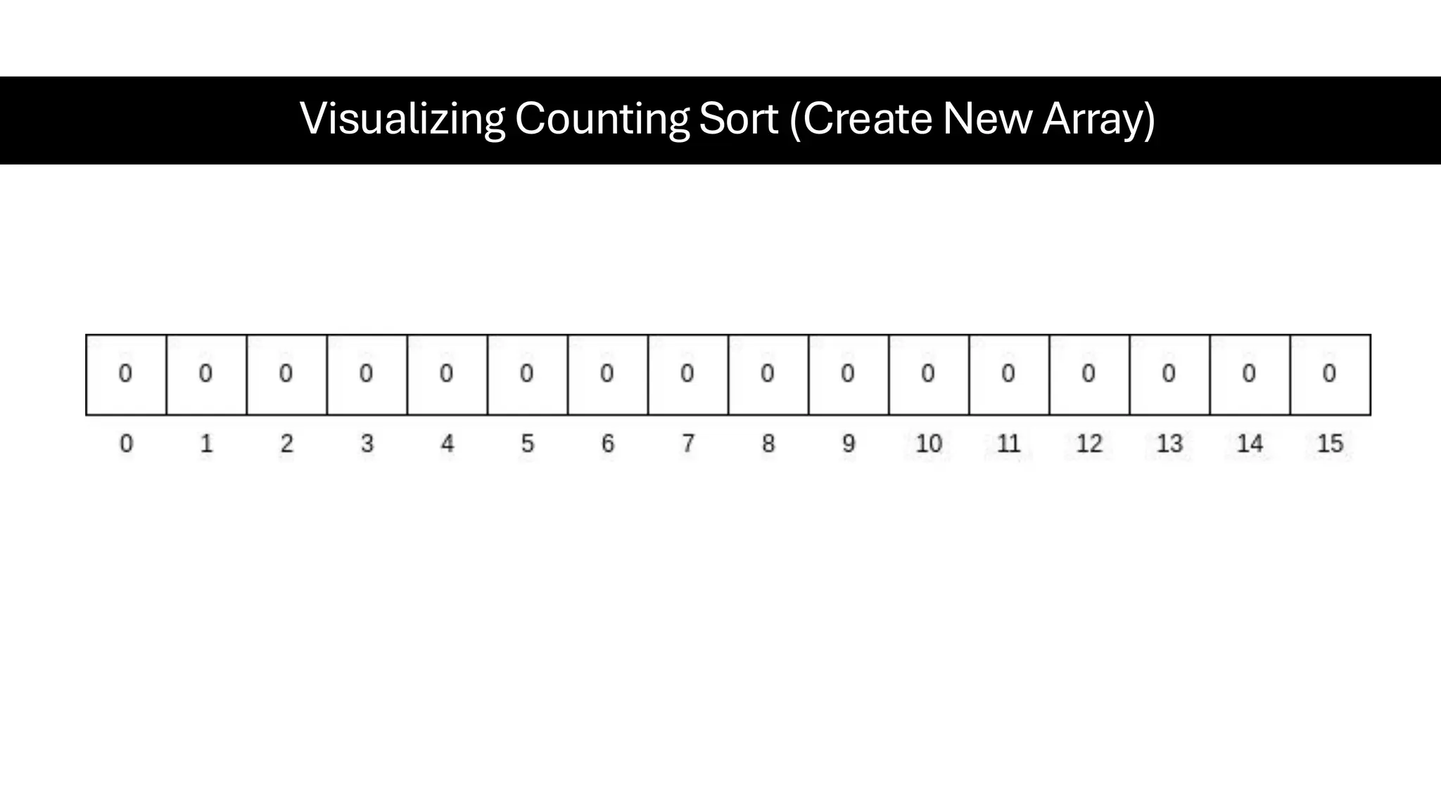
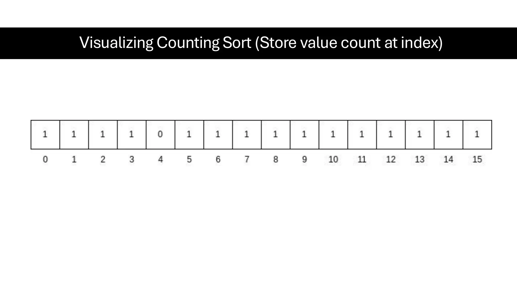
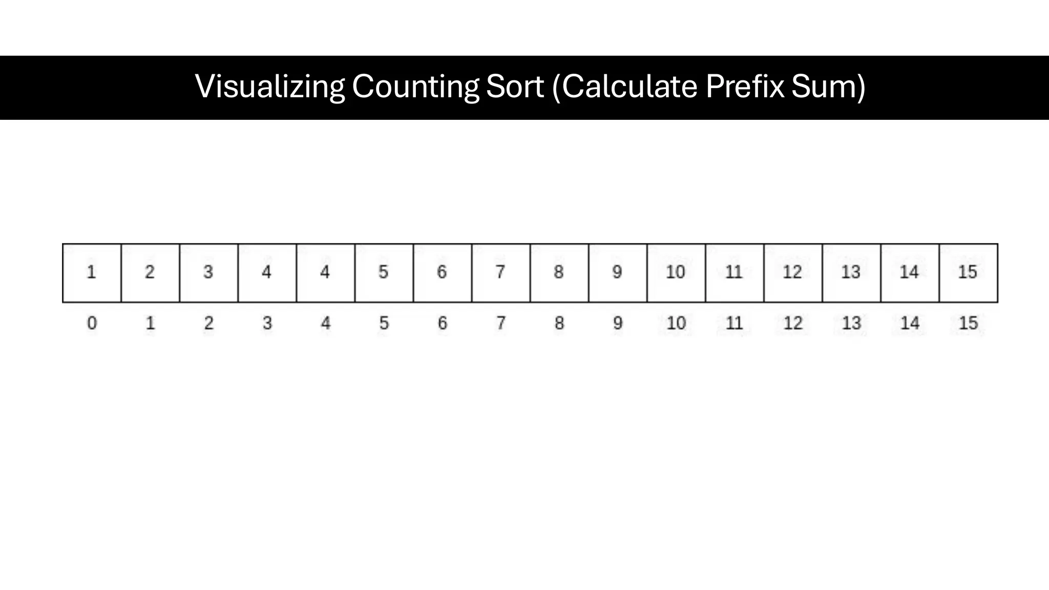
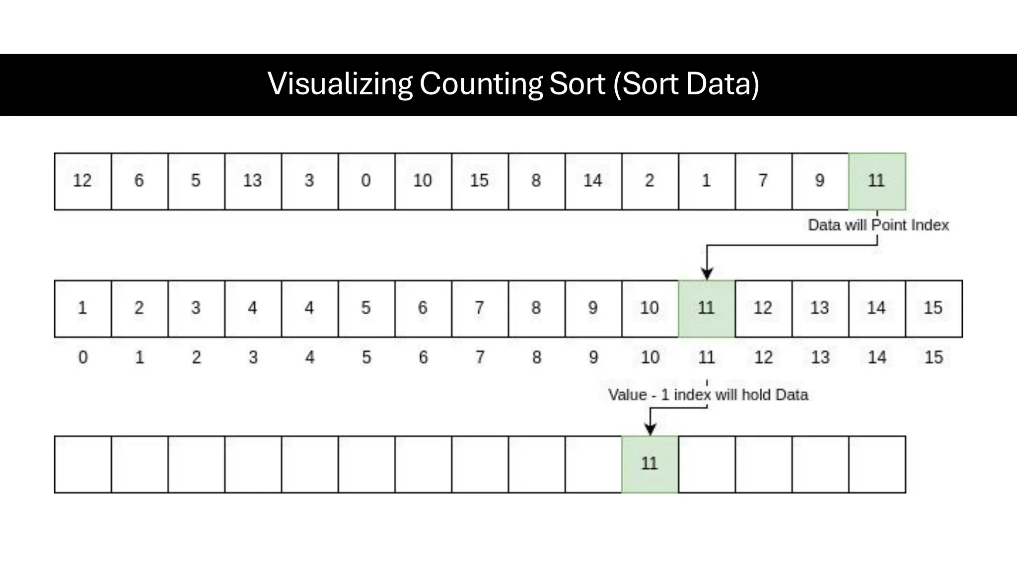
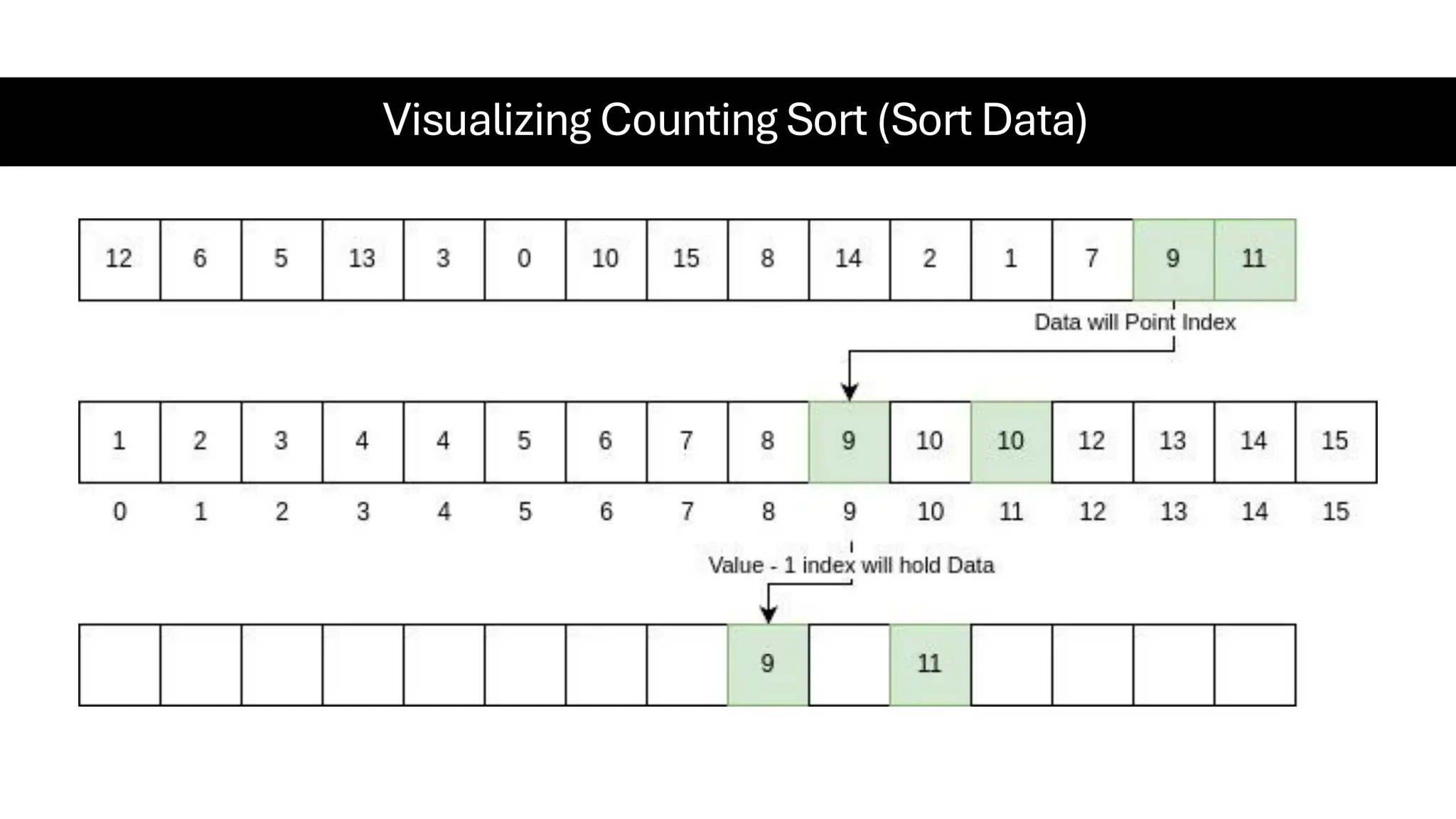
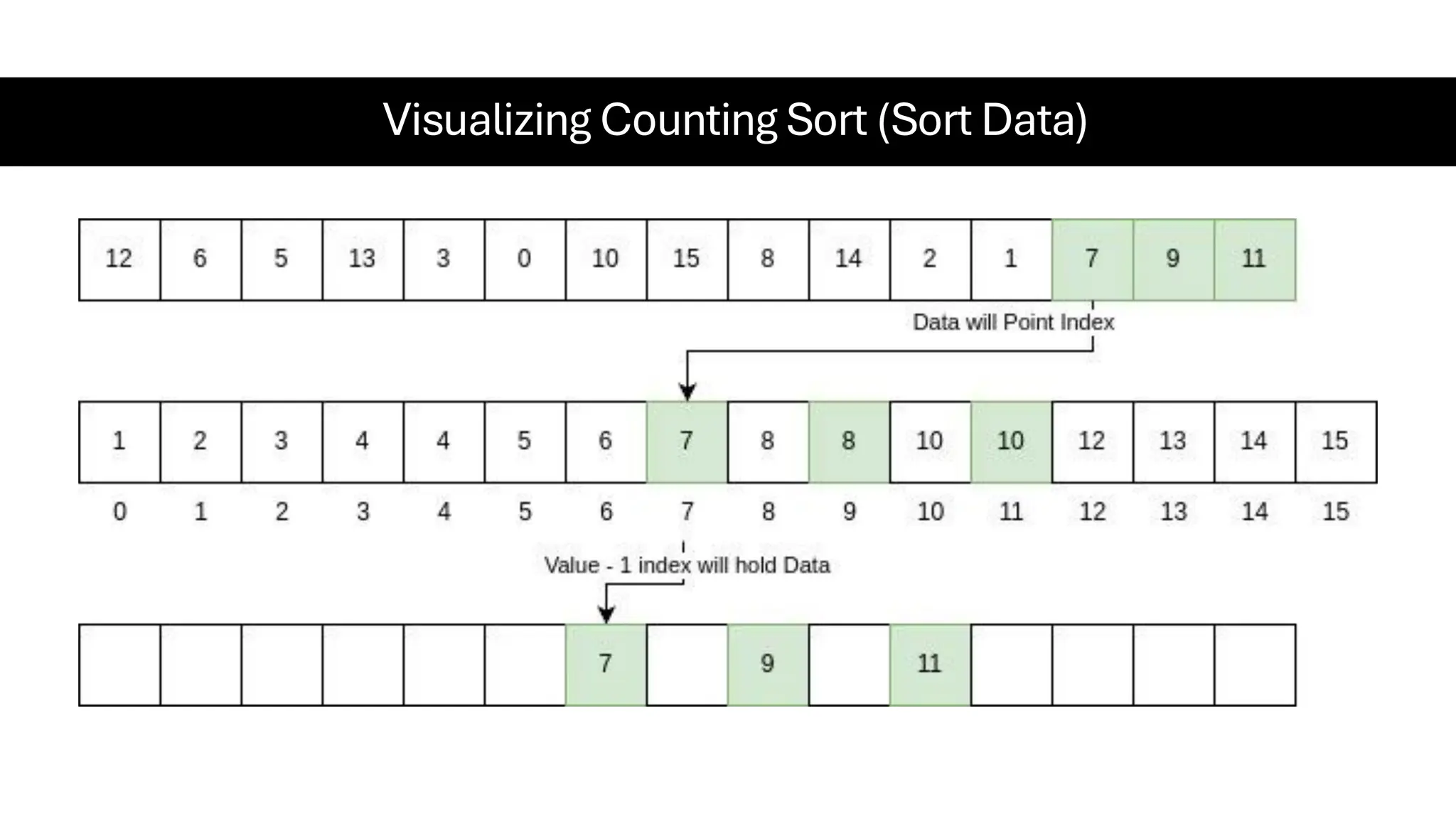
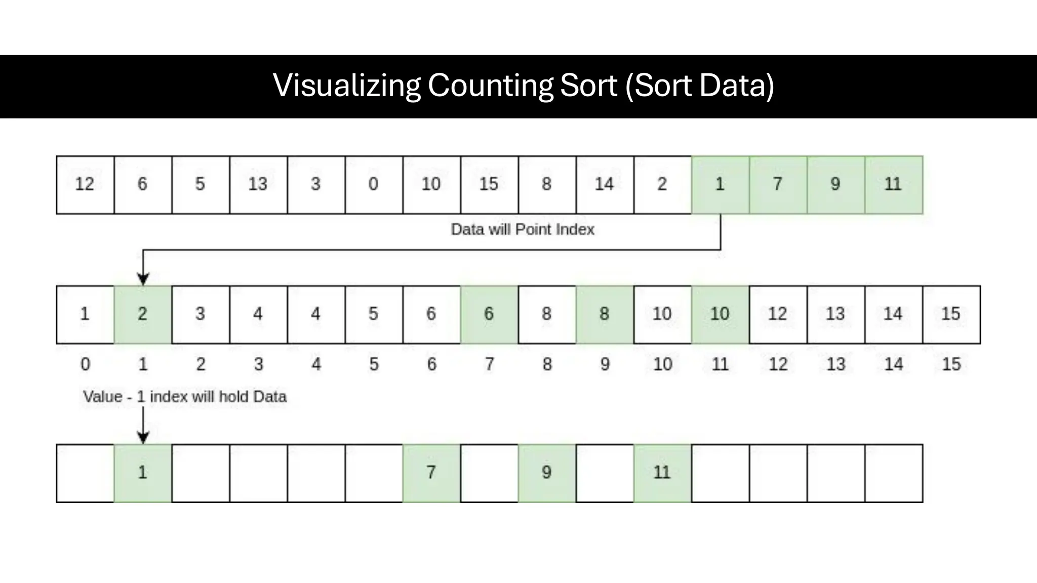
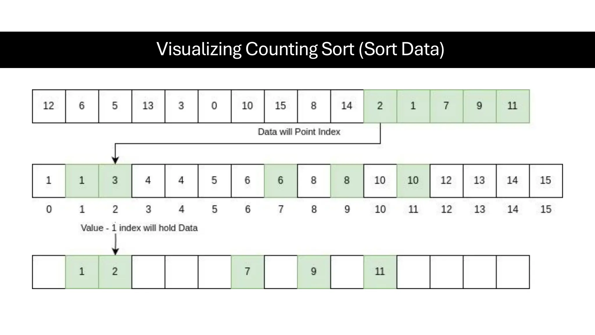
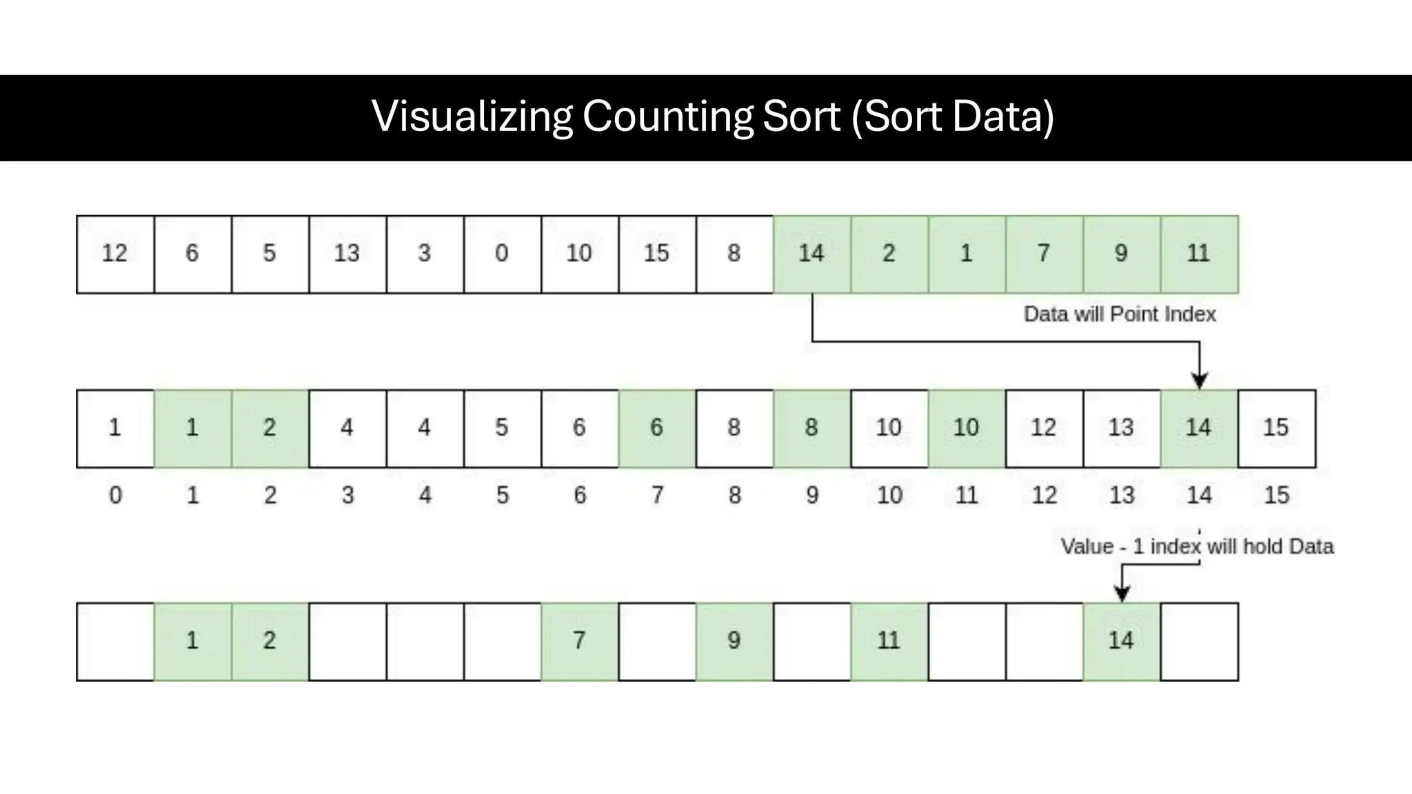
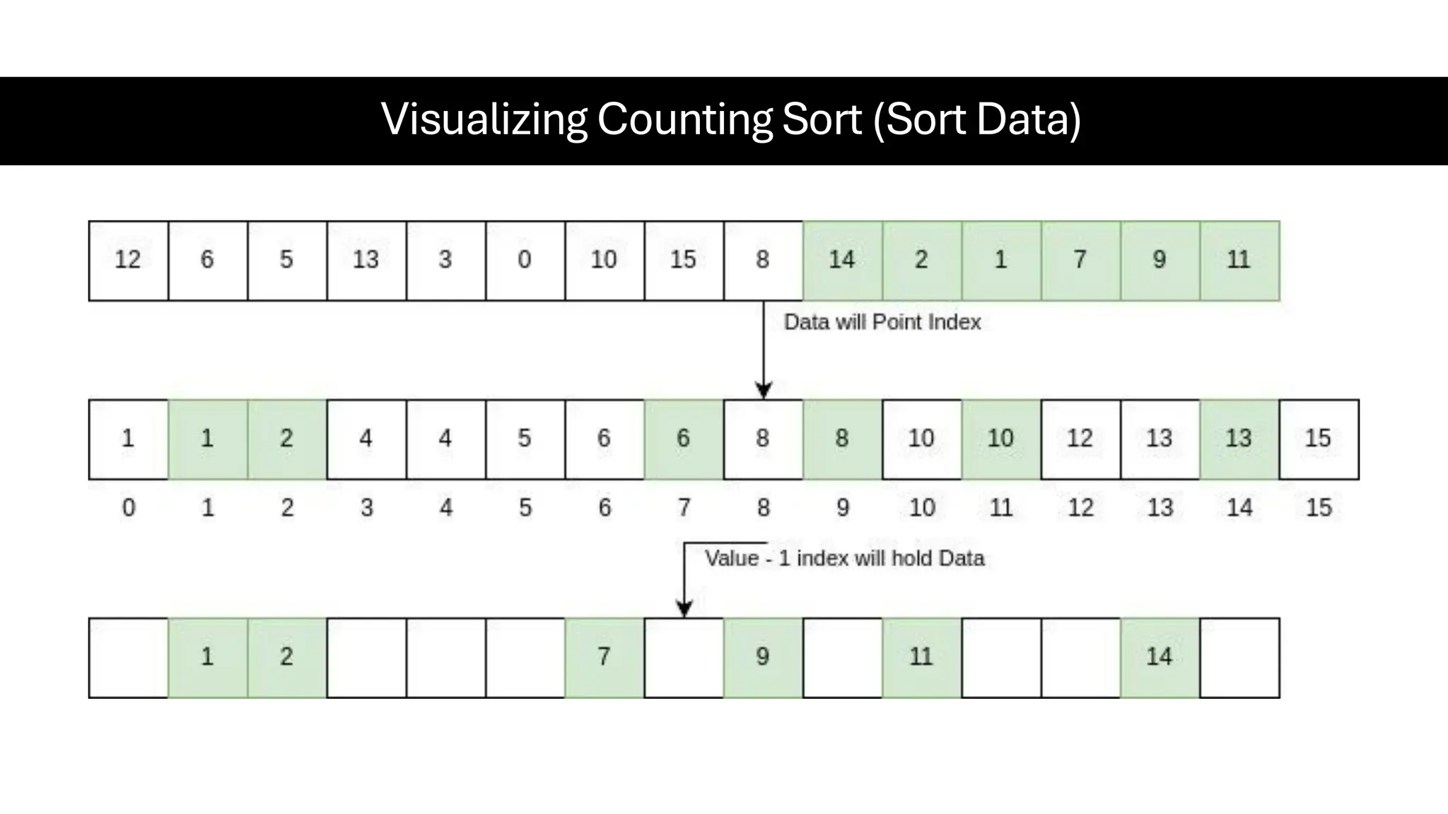
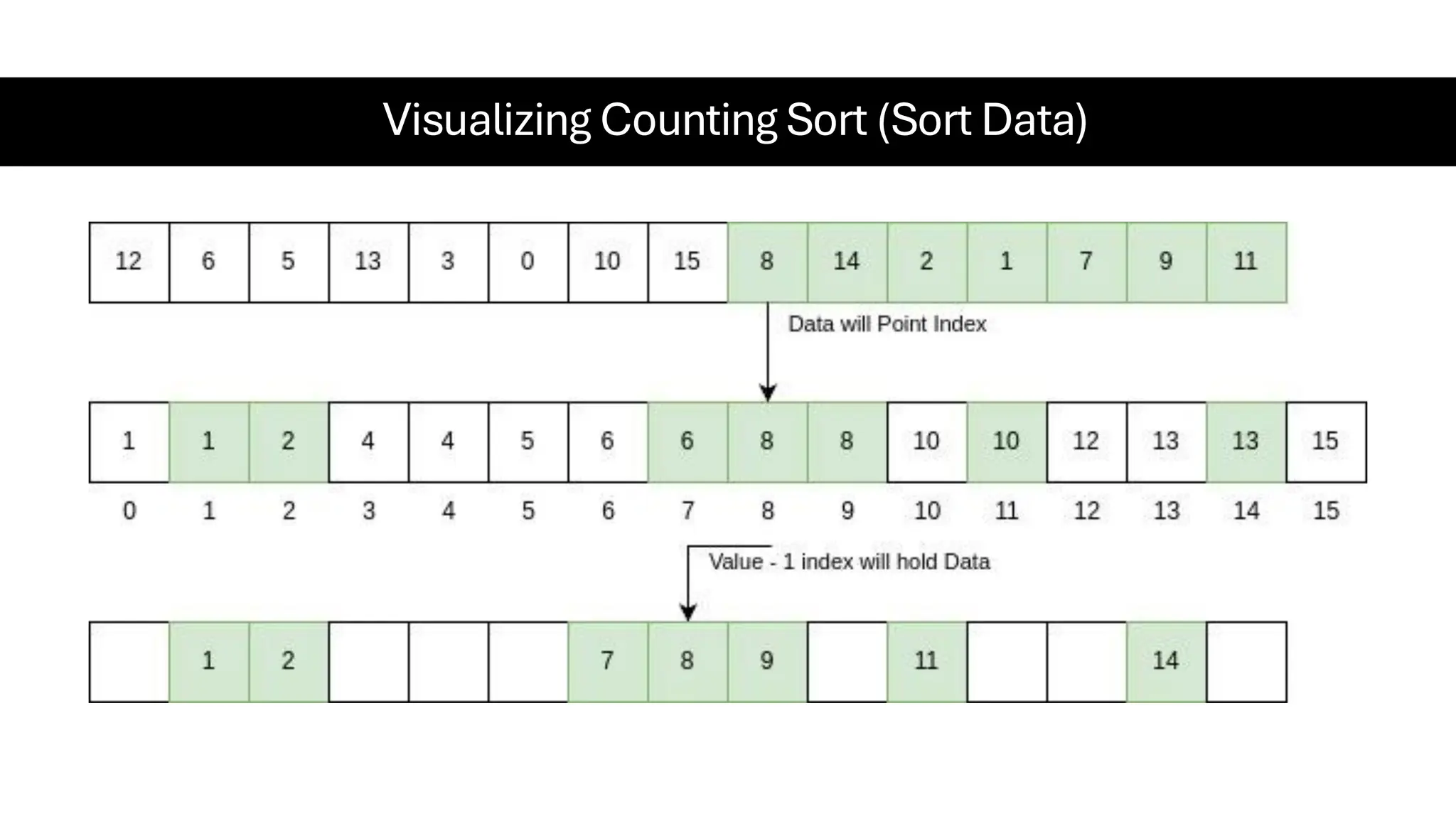
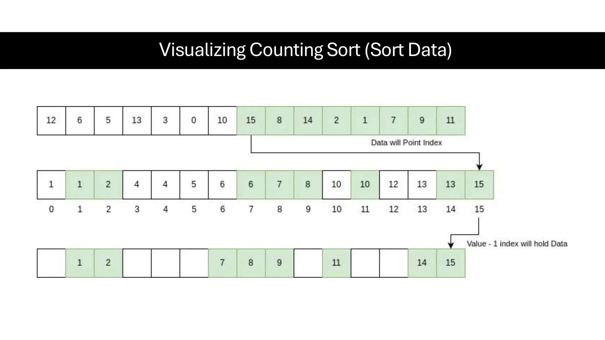
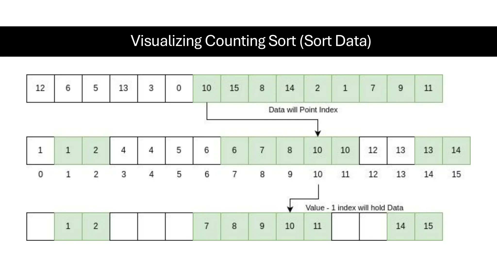
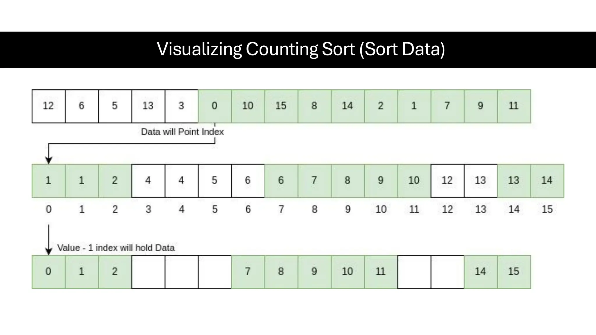
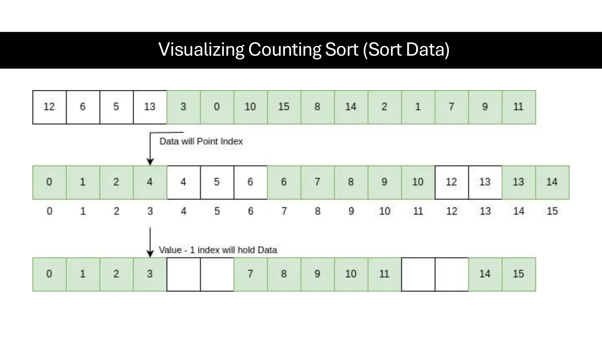
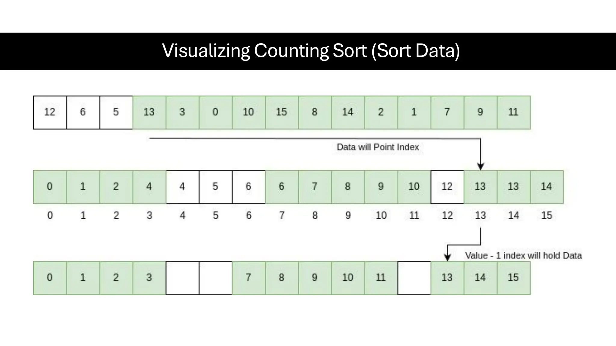
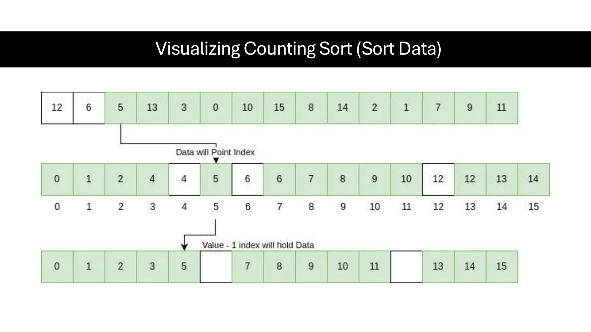
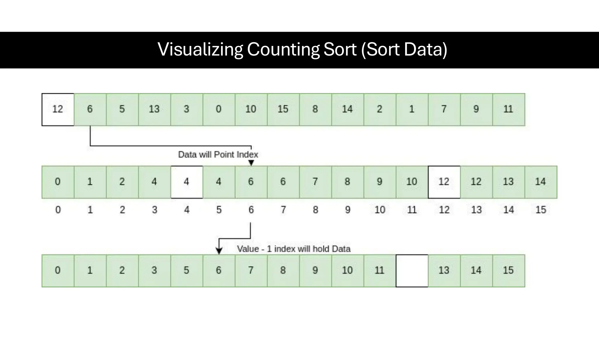
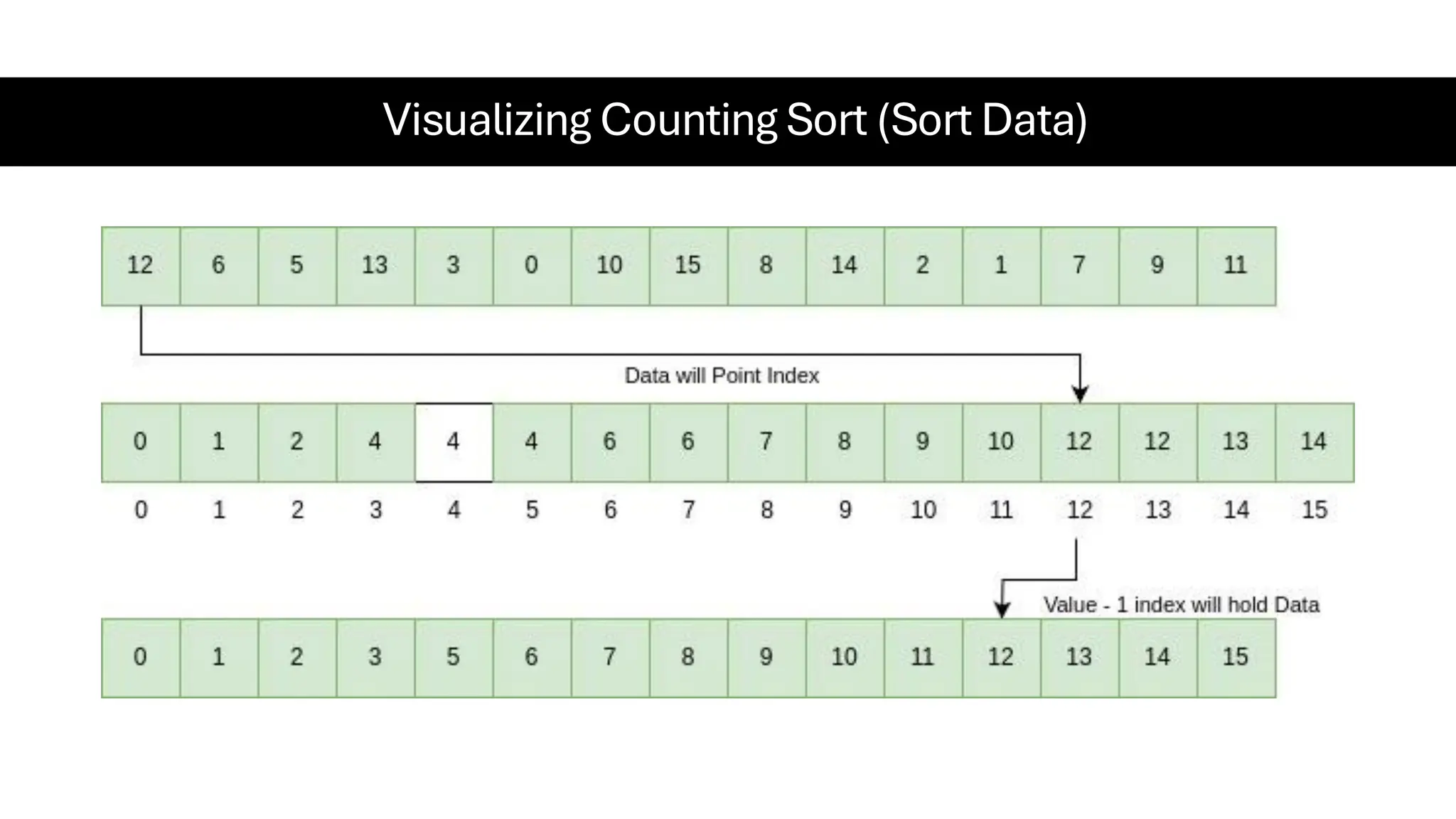
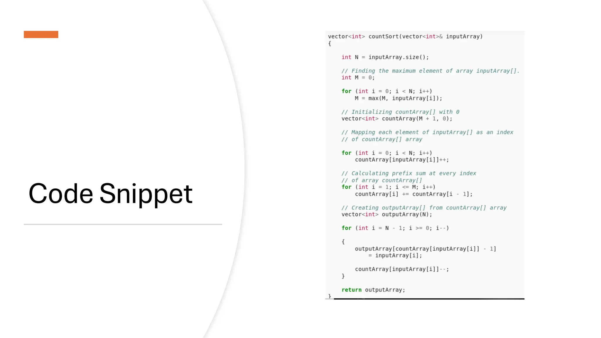
![Counting Sort • Counting Sort is a non-comparison-based sorting algorithm. It is particularly efficient when the range of input values is small compared to the number of elements to be sorted. The basic idea behind Counting Sort is to count the frequency of each distinct element in the input array and use that information to place the elements in their correct sorted positions. • Complexity Analysis of Merge Sort o Time Complexity: O(N+M), where N and M are the size of inputArray[] and countArray[] respectively. ▪ Worst-case: O(N+M). ▪ Average-case: O(N+M). ▪ Best-case: O(N+M). o Auxiliary Space: O(N+M), where N and M are the space taken by outputArray[] and countArray[] respectively.](https://image.slidesharecdn.com/datastructuresalgorithms-spring2025-250407112227-d7e7a1f6/75/Data-Structures-Algorithms-Spring-2025-pdf-318-2048.jpg)


This document is a comprehensive guide for the Data Structures & Algorithms course offered in Spring 2025. It covers key theoretical concepts, algorithmic strategies, and programming techniques, including recursion, sorting, dynamic programming, graph algorithms, and more. Designed for computer science undergraduates, the course material balances rigorous theory with practical problem-solving skills, preparing students for technical interviews and advanced coursework.