The document provides a comprehensive overview of data structures, including definitions, types, and operations associated with both primitive and non-primitive structures. Key topics include arrays, stacks, queues, linked lists, and algorithms for operations such as insertion, deletion, and sorting. Additionally, it covers memory representation, asymptotic notation for algorithm analysis, and specific concepts like sparse matrices and their representations.
Data Structure using ‘C’ Module- I Prepared by: Smruti Smaraki Sarangi Asst. Professor School of Computer Application IMS Unison University, Dehradun
2.
Topics Covered: Introductionto Data Structure Algorithm and Asymptotic Notation Array Sparse Matrix Stack Queue Linked List Polynomial Representation Dynamic Storage Management Compaction and Garbage Collection
3.
Introduction to DataStructure: It is the logical or mathematical model of a particular organization of data. It is the actual representation of data and the algorithms to manipulate the data. A programming construct used to implement Abstract Data Type (ADT). Abstract data type is a mathematical model or concept that defines a datatype correctly. It only mentions what operations are to be performed but not how these operations will be implemented. A data type is a term which refers to the kind of data that a variable may hold.
4.
Fundamental Concepts: Data:data are the raw facts. Information: Processed data is known as information. Entity: It is a thing or object in real world that distinguishable from all other objects. It is represented by set of attributes. Record: Collection of field values of a given entity. File: Collections of Records
5.
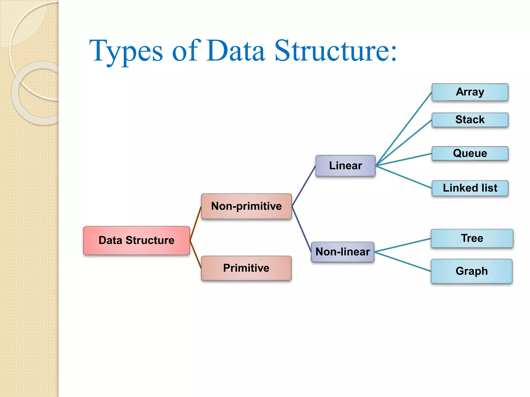
Types of DataStructure: Data Structure Non-primitive Linear Array Stack Queue Linked list Non-linear Tree GraphPrimitive
6.
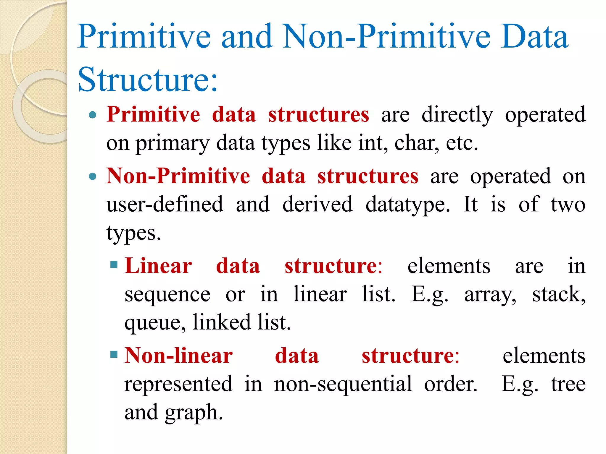
Primitive and Non-PrimitiveData Structure: Primitive data structures are directly operated on primary data types like int, char, etc. Non-Primitive data structures are operated on user-defined and derived datatype. It is of two types. Linear data structure: elements are in sequence or in linear list. E.g. array, stack, queue, linked list. Non-linear data structure: elements represented in non-sequential order. E.g. tree and graph.
7.
Operation on DataStructure: The operation performed on data structure are: Creation Insertion Deletion Search Traversal Sorting Merging
8.
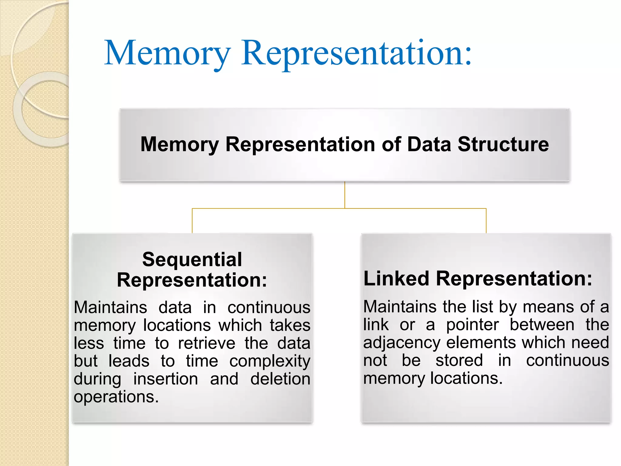
Memory Representation: Memory Representationof Data Structure Sequential Representation: Maintains data in continuous memory locations which takes less time to retrieve the data but leads to time complexity during insertion and deletion operations. Linked Representation: Maintains the list by means of a link or a pointer between the adjacency elements which need not be stored in continuous memory locations.
9.
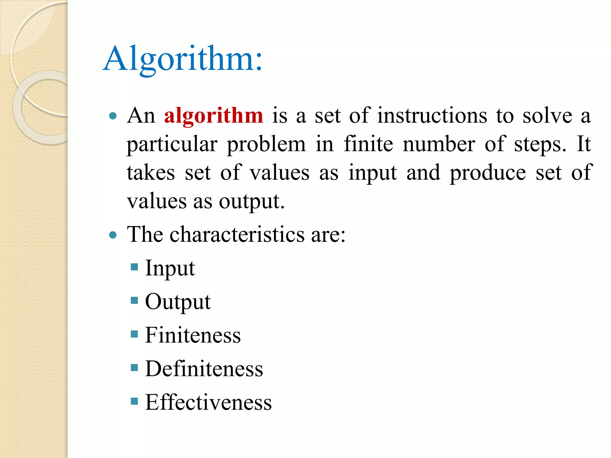
Algorithm: An algorithmis a set of instructions to solve a particular problem in finite number of steps. It takes set of values as input and produce set of values as output. The characteristics are: Input Output Finiteness Definiteness Effectiveness
10.
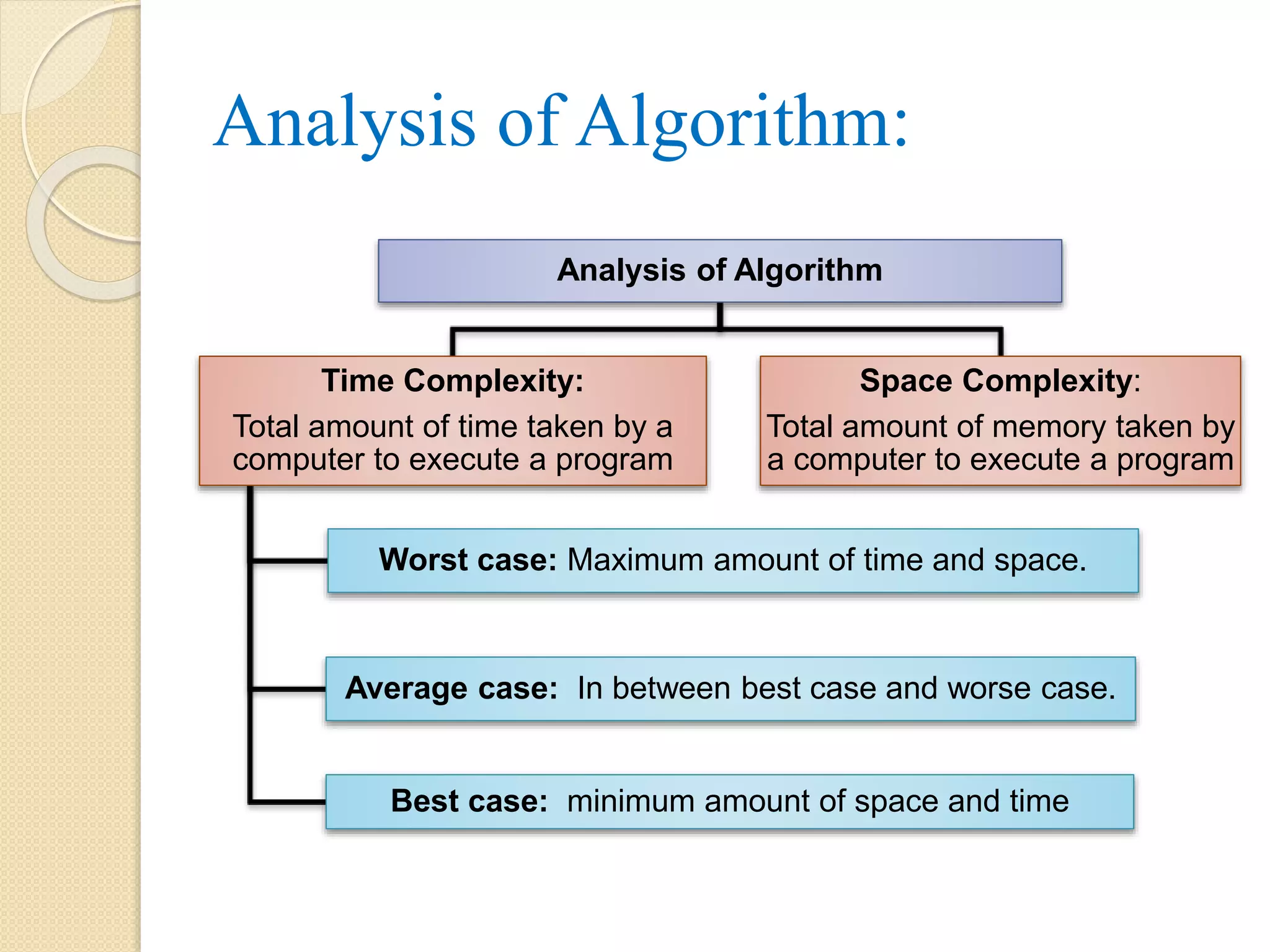
Analysis of Algorithm: Analysisof Algorithm Time Complexity: Total amount of time taken by a computer to execute a program Worst case: Maximum amount of time and space. Average case: In between best case and worse case. Best case: minimum amount of space and time Space Complexity: Total amount of memory taken by a computer to execute a program
11.
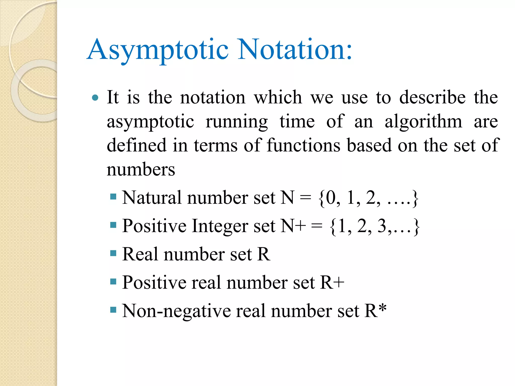
Asymptotic Notation: Itis the notation which we use to describe the asymptotic running time of an algorithm are defined in terms of functions based on the set of numbers Natural number set N = {0, 1, 2, ….} Positive Integer set N+ = {1, 2, 3,…} Real number set R Positive real number set R+ Non-negative real number set R*
12.
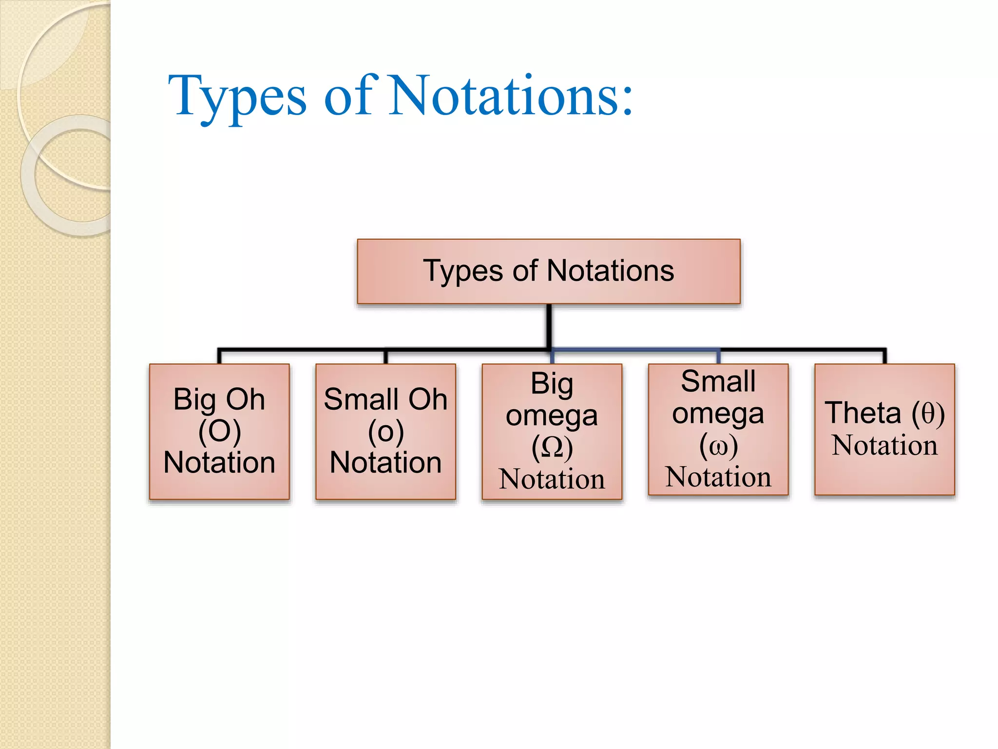
Types of Notations: Typesof Notations Big Oh (O) Notation Small Oh (o) Notation Big omega (Ω) Notation Small omega (ω) Notation Theta (θ) Notation
13.
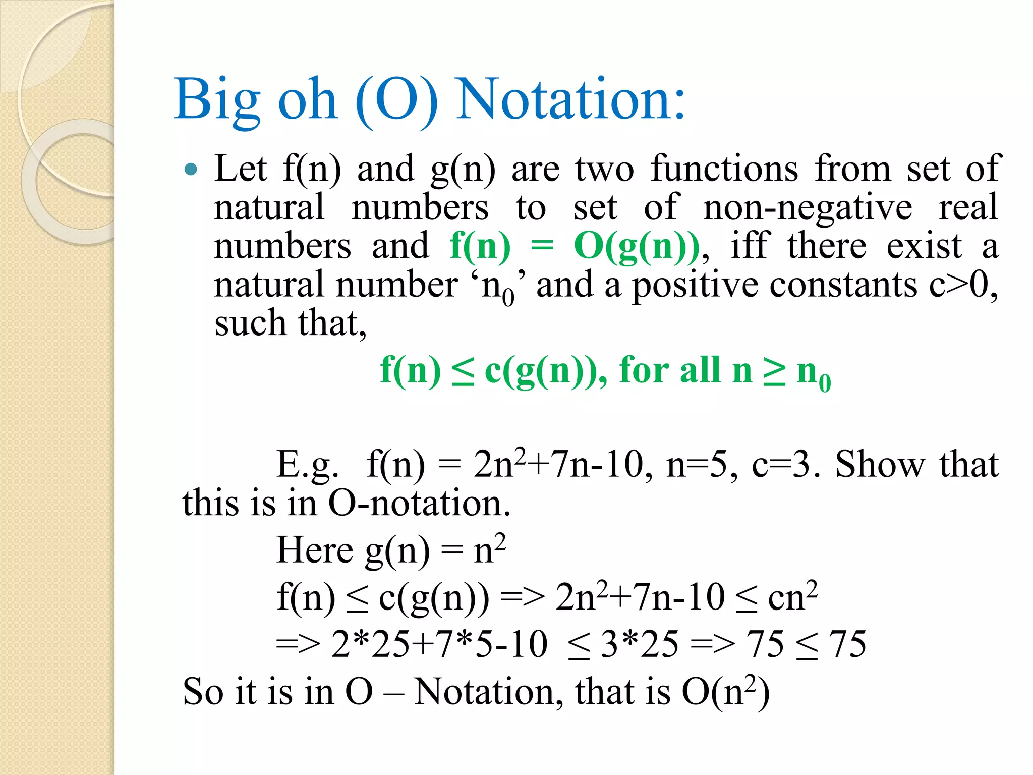
Big oh (O)Notation: Let f(n) and g(n) are two functions from set of natural numbers to set of non-negative real numbers and f(n) = O(g(n)), iff there exist a natural number ‘n0’ and a positive constants c>0, such that, f(n) ≤ c(g(n)), for all n ≥ n0 E.g. f(n) = 2n2+7n-10, n=5, c=3. Show that this is in O-notation. Here g(n) = n2 f(n) ≤ c(g(n)) => 2n2+7n-10 ≤ cn2 => 2*25+7*5-10 ≤ 3*25 => 75 ≤ 75 So it is in O – Notation, that is O(n2)
14.
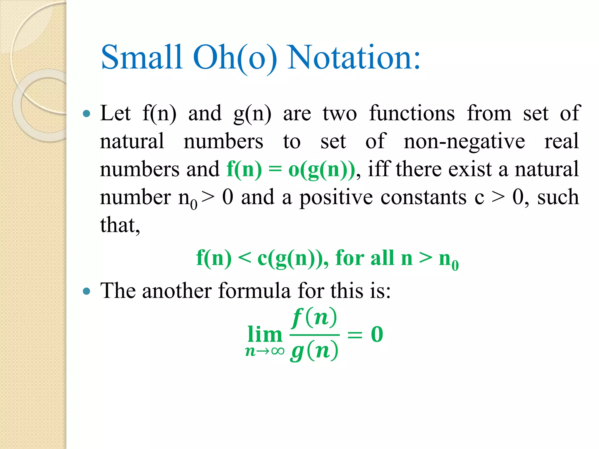
Small Oh(o) Notation: Let f(n) and g(n) are two functions from set of natural numbers to set of non-negative real numbers and f(n) = o(g(n)), iff there exist a natural number n0 > 0 and a positive constants c > 0, such that, f(n) < c(g(n)), for all n > n0 The another formula for this is: 𝐥𝐢𝐦 𝒏→∞ 𝒇 𝒏 𝒈 𝒏 = 𝟎
15.
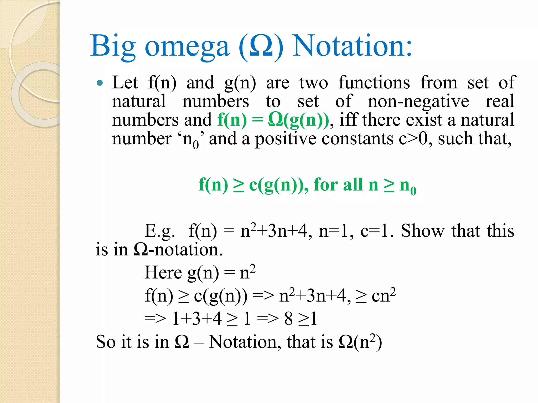
Big omega (Ω)Notation: Let f(n) and g(n) are two functions from set of natural numbers to set of non-negative real numbers and f(n) = Ω(g(n)), iff there exist a natural number ‘n0’ and a positive constants c>0, such that, f(n) ≥ c(g(n)), for all n ≥ n0 E.g. f(n) = n2+3n+4, n=1, c=1. Show that this is in Ω-notation. Here g(n) = n2 f(n) ≥ c(g(n)) => n2+3n+4, ≥ cn2 => 1+3+4 ≥ 1 => 8 ≥1 So it is in Ω – Notation, that is Ω(n2)
16.
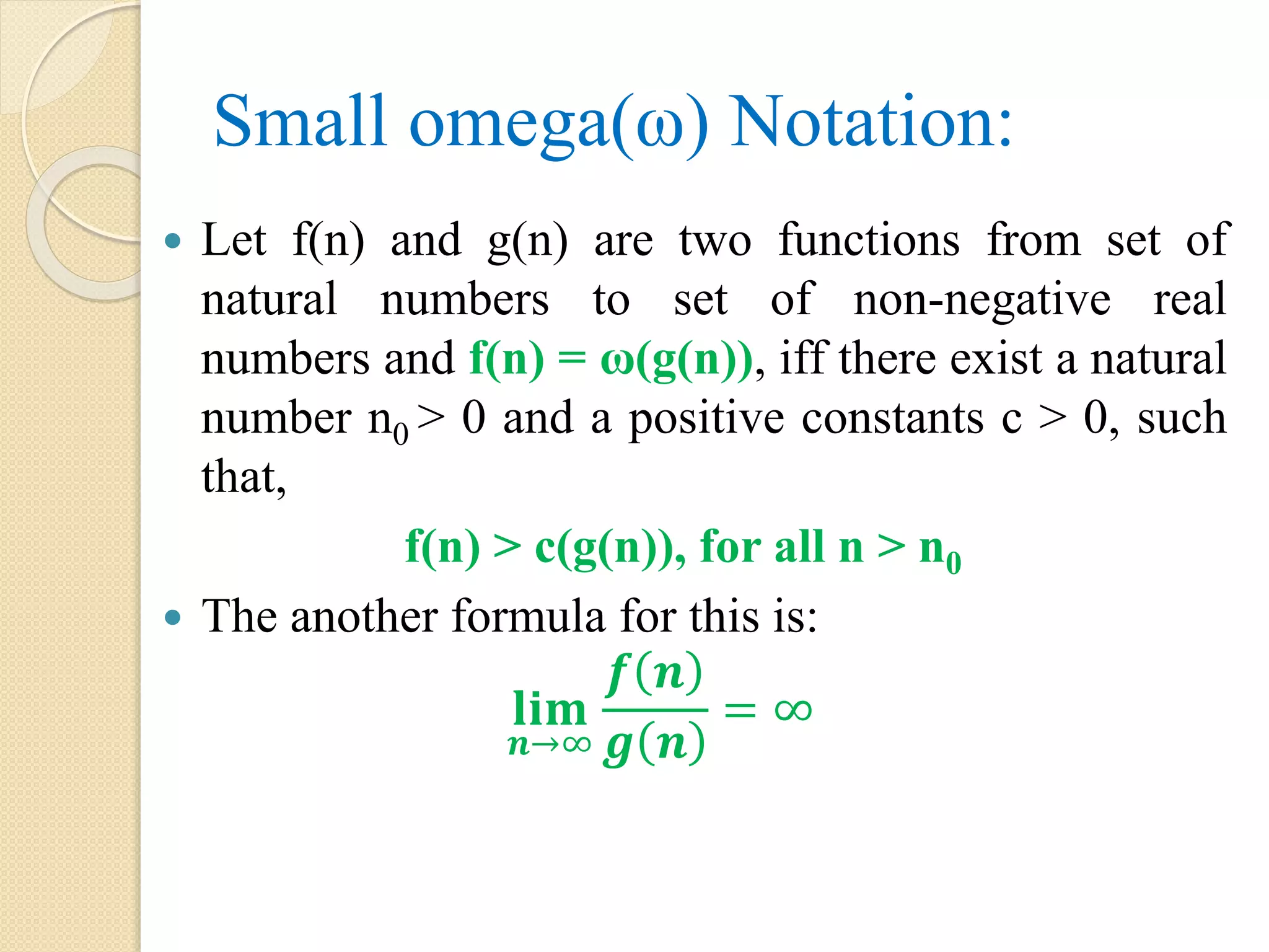
Small omega(ω) Notation: Let f(n) and g(n) are two functions from set of natural numbers to set of non-negative real numbers and f(n) = ω(g(n)), iff there exist a natural number n0 > 0 and a positive constants c > 0, such that, f(n) > c(g(n)), for all n > n0 The another formula for this is: 𝐥𝐢𝐦 𝒏→∞ 𝒇 𝒏 𝒈 𝒏 = ∞
17.
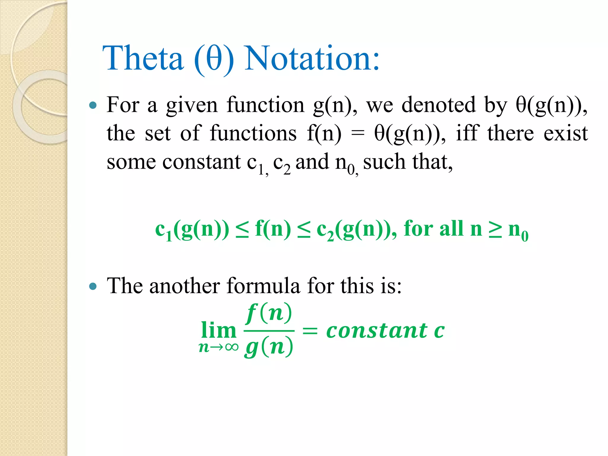
Theta (θ) Notation: For a given function g(n), we denoted by θ(g(n)), the set of functions f(n) = θ(g(n)), iff there exist some constant c1, c2 and n0, such that, c1(g(n)) ≤ f(n) ≤ c2(g(n)), for all n ≥ n0 The another formula for this is: 𝐥𝐢𝐦 𝒏→∞ 𝒇 𝒏 𝒈 𝒏 = 𝒄𝒐𝒏𝒔𝒕𝒂𝒏𝒕 𝒄
18.
Array: It isa collection of similar data elements present in continuous memory locations referred by a unique name. It can be one dimensional, two dimensional and multidimensional array. Two dimensional array has 2 subscripts one for row and other for column. It is also called matrix.
19.
One-Dimensional Array: Alinear array is a list of finite number ‘n’ of homogeneous data element, such that: The elements of the array are referred respectively by an index set consisting of ‘n’ consecutive numbers. The elements of the array are stored respectively in successive memory location. It can be defined as: datatype arrayname[size];
20.
The number‘n’ of elements is called the length or size of the array. The length of an array can be obtained from the index by the formula: Length = Upperbound(UB) – Lowerbound(LB)+1 where UB = Largest index and LB = Smallest Index of array. When Lowerbound = 1, then Length = Upperbound(UB)
21.
Operations of 1DArray: The operations of one dimensional array are: Creation: create or entering elements into array. Traversal: processing each element Search: searching for an element Insertion: inserting an element at required position Deletion: deletion of an element Sorting: arranging in ascending or descending order Merging: concatenate two ways into 3rd array or merge directly into 3rd array where two arrays are already sorted.
22.
Creation of anArray: Algorithm: CREATE(LA, LB, UB) Step 1: Let LA[10], LB,UB, K Step 2: LB = 1, UB = 10 Step 3: Display “enter 10 elements” Step 4: Repeat, for K = LB to UB incremented by INPUT LA[K] [End of for] Step 5: Exit (LA: linear array, LB: Lower Bound, UB: Upper Bound)
23.
Traversing an Array: Algorithm: TRAVERSE(LA,LB,UB) Step 1: Repeat for K = LB to UB by 1 Apply PROCESS to LA[K] Step 2: Exit (LA: linear array, LB: Lower Bound, UB: Upper Bound)
24.
Searching for anelement in an Array: Algorithm: SEARCH(LA,LB,UB,ITEM) Step 1: Let K, Set K = LB Step 2: Repeat, while(K < = UB) •Step 2.1: If LA[K] = ITEM, then Display “Item found at”, K [End of if] Step 2.2: Set K = K + 1 (End of while) Step 3: Exit (LA: linear array, LB: Lower Bound, UB: Upper Bound)
25.
Insertion of newelement in an Array: Algorithm: INSERTION(LA,LB,UB,ITEM,POS) Step 1: Let K Step 2: Repeat for K = UB to POS, decreasing by 1 LA[K + 1] = LA[K] [End of for] Step 3: LA[POS] = ITEM Step 4: Set LB = UB + 1 Step 5: Exit (LA: linear array, LB: Lower Bound, UB: Upper Bound, POS = position)
26.
Deletion of anelement from Array: Algorithm for deletion when position is given: DELETION_POS(LA, LB,UB,POS) Step 1: Let K Step 2: Repeat for K = POS to UB incremented by 1 LA[K] = LA[K + 1] [end of for] UB = UB - 1 Step 3: Exit (LA: linear array, LB: Lower Bound, UB: Upper Bound, POS = position)
27.
Deletion of anelement from Array: Algorithm for deletion when item is given: DELETION_ITEM(LA, LB,UB,ITEM) Step 1: Let K, S = 0, T Step 2: Repeat for K = LB to UB incremented by 1 Step 2.1:If (LA[K] = ITEM), then Step 2.1.1: Display “ITEM found at”, K Step 2.1.2: Repeat for T = K to UB, incremented by 1 Step 2.1.2.1: LA[T] = LA[T + 1] [End of for] Step 2.1.3: UB = UB - 1 Step 2.1.4: S-1 [end of if] [End of for] Step 3: If (S=0), then Step 3.1: Display “ITEM to be deleted is not found” [End of if] Step 4: Exit (LA: linear array, LB: Lower Bound, UB: Upper Bound)
28.
Sorting the elementsof an Array: Algorithm: SORTING(LA,LB,UB) Step 1: Let I, J, K, T Step 2: Set I = 1, J = 2 Step 3: Repeat for K = UB – 1 to 1 by decrementing by 1 Step 3.1: Repeat for I = 1, J = 2 to K by 1 Step 3.1.1: If LA[I] > LA[J], then T = LA[I] LA[I] = LA[J] LA[J] = T [End of if] [End of for] [End of for] Step 4: Exit (LA: linear array, LB: Lower Bound, UB: Upper Bound)
29.
Two-Dimensional Array: Twodimensional array is the array which is represented by two dimensions that is row and column. The declaration of two dimensional array is: datatype arrayname[row size][column size]; The two dimensional array is also called as Matrix.
30.
Memory Representation of2D Array: The programming language will store the two dimensional array ‘A’ in two different ways. That is: Row-Major Order (Row by Row) Column- Major Order (Column by Column)
31.
Row-Major Order (Rowby Row): In Row–Major order, elements of 2D array are stored on a row-by-row basis beginning from first row. Address of an element represented in row-major order can be calculated by using the following formula: Address of A[i][j] = B + W * [(N * (i - LBR)) +(j - LBC)] If LBR = LBC = 0, then the formula can be represented as: Address of A[i][j] = B + W* (N * i + j)]
32.
Example: [Row-Major Order Representation] B= base address = 100, W = datatype value of the array N = size of column, i = row index value, j = column index value LBR = lower bound row, LBC = lower bound column Address of A[1][3] = 100 + 2 * [(4 * 1 – 0) + (3 – 0)] = 100 + 2 * [(4 * 1) + 3] = 100 + 2 * 7 = 114 7 9 20 1 11 5 2 17 13 15 21 19 Data in array 0,0 0,1 0,2 0,3 1,0 1,1 1,2 1,3 2,0 2,1 2,2 2,3 Row and column values
33.
Column-Major Order (Columnby Column): In Column–Major order, elements of 2D array are stored on a column-by-column basis beginning from first column. Address of an element represented in column-major order can be calculated by using the following formula: Address of A[i][j] = B + W * [(i - LBR) + M * (j - LBC)] If LBR = LBC = 0, then the formula can be represented as: Address of A[i][j] = B + W* (i + M * j)]
34.
Example: [Column-Major Order Representation] B= base address = 100, W = datatype value of the array M = size of row, i = row index value, j = column index value LBR = lower bound row, LBC = lower bound column Address of A[1][3] = 100 + 2 * [(1 – 0) +3 * (3 – 0)] = 100 + 2 * [1 + 9] = 100 + 20 = 120 7 11 13 9 5 15 20 2 21 1 17 19 Data in array 0,0 0,1 0,2 1,0 1,1 1,2 2,0 2,1 2,2 3,0 3,1 3,2 Column and Row values
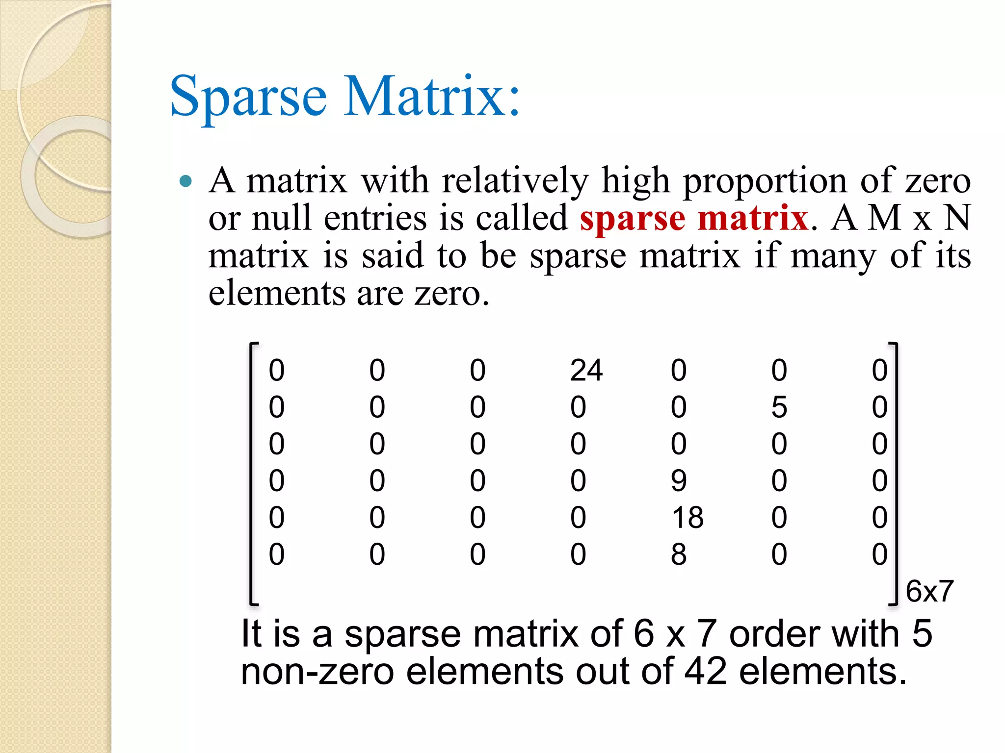
Sparse Matrix: Amatrix with relatively high proportion of zero or null entries is called sparse matrix. A M x N matrix is said to be sparse matrix if many of its elements are zero. 0 0 0 24 0 0 0 0 0 0 0 0 5 0 0 0 0 0 0 0 0 0 0 0 0 9 0 0 0 0 0 0 18 0 0 0 0 0 0 8 0 0 6x7 It is a sparse matrix of 6 x 7 order with 5 non-zero elements out of 42 elements.
37.
Array Representation ofSparse Matrix: The alternate data structure that we consider to represent a sparse matrix is a triplet. The triplet is a 2D array having t+1rows and 3 columns, where t is the total number of non-zero entries. The first row of the triplet contains number of rows, columns and non-zero entries available in the matrix in its 1st, 2nd, and 3rd column respectively.
38.
In addition,we need to record the size of matrix, that is number of rows and number of columns and non-zero elements. For this purpose, the first element of array of triplets is used where the first field stores number of rows and second field stores number of columns and third field stores number of non- zero elements.
39.
Possible Operations ofSparse Matrix: To store the non-zero entries of a sparse matrix into alternate triplet representation. To display the original matrix from a given triplet representation of matrix. To store transpose of the triplet representation. To display the transpose of original sparse matrix using transpose of triplet.
Algorithm for operationson Sparse Matrix: Step 1: Let A[10][10], SP[50[3], TP[5][3], I, J, M, N, NZ Step 2: NZ = 0 Step 3: Display “ Enter the row and column size”. Step 4: Input M,N Step 5: Repeat for I = 0 to M – 1 incremented by 1 Step 5.1: Repeat for J = 0 to N – 1 incremented by 1 Input A[I][J] if A[I][J] != 0, then NZ = NZ + 1 [End of if] [End of Step 5.1]
42.
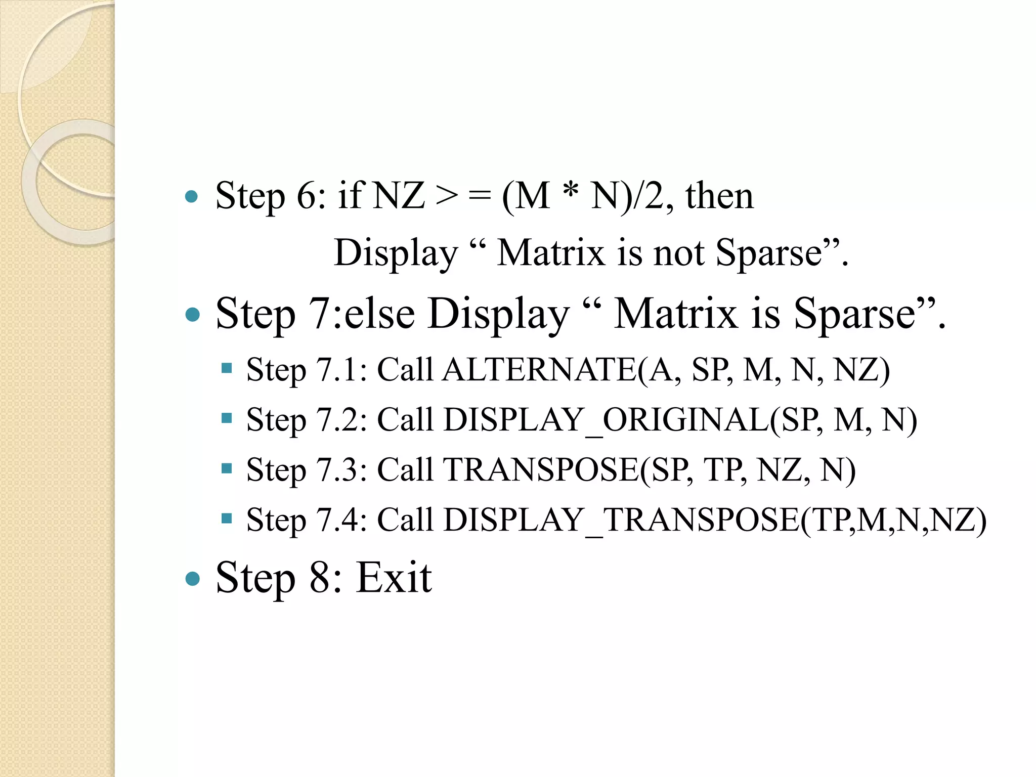
Step 6:if NZ > = (M * N)/2, then Display “ Matrix is not Sparse”. Step 7:else Display “ Matrix is Sparse”. Step 7.1: Call ALTERNATE(A, SP, M, N, NZ) Step 7.2: Call DISPLAY_ORIGINAL(SP, M, N) Step 7.3: Call TRANSPOSE(SP, TP, NZ, N) Step 7.4: Call DISPLAY_TRANSPOSE(TP,M,N,NZ) Step 8: Exit
43.
Algorithm to Representa Sparse Matrix to Triplet Matrix: ALTERNATE(A, SP, M, N, NZ) Step 1: Let I, J, K = 1 Step 2: SP[0][0] = M, SP[0][1] = N, SP[0][2] = NZ Step 3: Repeat for I = 0 to M – 1 incremented by 1 Step 3.1: Repeat for J = 0 to N – 1 incremented by 1 if A[I][J] != 0 then SP[K][0] = I SP[K][1] = J SP[K][2] = A[I][J] K = K + 1 [End of if] [End of Step 3.1] Step 4: Repeat for K = 0 to NZ incremented by 1 Display SP[K][0], SP[K][1], SP[K][2] [End of for] Step 5: Exit
44.
Algorithm to displayoriginal matrix using triplet: DISPLAY_ORIGINAL(SP, M, N) Step 1: Let I, J, K Step 2: K = 1 Step 3: Repeat for I = 0 to M – 1 increased by 1 Step 3.1: Repeat for J = 0 to N – 1 increased by 1 if(SP[K][0] = I AND SP[K][1] = J), then Display SP[K][2] K = K + 1 else Display “0” [End of if] [End of for step 3.1] [End of for step 3] Step 4: Exit
45.
Transpose of tripletmatrix into alternate matrix: TRANSPOSE(SP, TP, NZ, N) Step 1: Let J, K, T = 1 Step 2: TP[0][0] = SP[0][1], TP[0][1] = SP[0][0], TP[0][2] = SP[0][2]. Step 3: Repeat for I = 0 to M – 1 incremented by 1 Step 3.1: Repeat for J = 0 to N – 1 incremented by 1 if(SP[K][1] = J), then TP[T][0] = SP[K][1] TP[T][1] = SP[K][0] TP[T][2] = SP[K][2] T = T + 1 [End of if] Step 4:Repeat for T = 0 to NZ – 1 incremented by 1 Display TP[T][0], TP[T][1], TP[T][2] [End of for] Step 5: Exit
46.
Display transpose oforiginal matrix using transpose of triplet: DISPLAY_TRANPOSE(TP, M, N, NZ) Step 1: Let I, J, T Step 2: T = 1 Step 3: Repeat for J = 0 to N – 1 incremented by 1 Step 3.1: Repeat for I = 0 to M – 1 incremented by 1 if(TP[T][0] = J AND TP[T][1] = I), then Display TP[T][2] T = T + 1 else Display “0” [End of if] [End of for step 3.1] [End of for step-3] Step 4: Exit
47.
STACK: It isa non-primitive linear data structure, which works on the concept of Last In First Out (LIFO) or First in Last Out (FILO). It is an ordered list, where insertion and deletion can be done at one end only, which is called TOP element of the stack. The operations of stack are: PUSH(insertion), POP(deletion) and PEEP(display location) E.g. i) stack of plates one above the other. ii) stack of books kept one above the other.
48.
Memory Representation ofStack: Array Representation: An one dimensional array can be considered for representing a stack in memory. While representing a stack in the form of an array we take a variable TOP that identifies top most element of the stack. Initially, when the stack is empty TOP = -1. The operation of pushing an ITEM into a stack and the operation of removing an ITEM from the stack is done by PUSH and POP. In executing the procedure PUSH, one must first test whether there is room in the stack for new ITEM, if not then we have the condition known as “OVERFLOW”.
49.
The conditionfor overflow is TOP = SIZE – 1, where SIZE is the maximum number of elements that can be hold by the array that represents the stack in memory. In executing the procedure POP, we must first test whether there is an element in the stack to be deleted, if not then we have the condition known as “UNDERFLOW”. The condition for this is TOP = -1. Linked Representation: The concept of dynamic memory allocation is implemented by using linked list to represent stack in linked format.
50.
Algorithm for PUSHOperation: PUSH(STACK, TOP, SIZE, ITEM) Step 1: if (TOP = SIZE -1), then Display “Overflow” Exit Step 2: else TOP = TOP + 1 STACK[TOP] = ITEM [End of if] Step 3: Exit
51.
Algorithm for POPOperation: Step 1: Let ITEM Step 2: if (TOP < 0), then Display “Underflow” Exit Step 3: else ITEM = STACK[TOP] Display “popped item is”, ITEM TOP = TOP - 1 [End of if] Step 4: Exit
52.
Algorithm for PEEPOperation: Step 1: if TOP = -1, then print “Underflow” and return Step 2: Read the location value ‘i’ Step 3: Return the ith element from the top of the stack. Return(STACK(K[TOP – i + 1]) Algorithm for UPDATE Operation: UPDATE(STACK, ITEM) Step 1: if TOP = -1, then print “Underflow” and return Step 2: Read the location value ‘i’ Step 3: STACK[TOP – i + 1] Step 4: Return
53.
Applications of Stack: Stacks are used to pass parameter between functions on a call to a function the parameters and local variable are stored on a stack. High level programming language, such as ‘pascal’, ‘c’, that provides for recursion used stack for book keeping. That is: in each recursive call, there is need to save the current values of parameter local variables and return address.
54.
Conversion and Evaluationof Arithmetic Expression: Arithmetic Expression Notation: In any arithmetic expression, each operator is placed in between two operands i.e. mathematical expression is called as infix expression. E.g.: A + B. Apart from usual mathematical representation of an arithmetic expression, an expression can also be represented in the following two ways. i.e. i) Polish or Prefix Notation ii) Reverse Polish or Postfix Notation
55.
Mathematical Procedure forConversion: Standard Arithmetic Operators and Precedence levels are: ^ (exponential): Higher level *, /, % : Middle Level +, - : Lower Level The possible conversions are: Infix to Prefix Prefix to Infix Infix to Postfix Postfix to Infix Prefix to Postfix Postfix to Prefix
56.
Infix to Prefix: Identify the innermost bracket Identify the operator according to the priority of evaluation. Represent the operator and corresponding operand in prefix notation Continue this process until the equivalent prefix expression is achieved. E.g.: (A + B * (C – D ^ E) / F) => (A + B * (C – [^DE]) / F) => (A + B * [ - C ^ DE] / F) => (A + [* B – C ^ DE] / F) => A + [/ * B – C ^ DEF] => + A / * B – C ^ DEF
57.
Prefix to Infix: Identify the operator from right to left order. The two operands which immediately follows the operator are for evaluation. Represent the operator and corresponding operand in infix notation Continue this process until the equivalent infix expression is achieved. If the priority of a scanned operator is less than any operators available with [], then put them within (). E.g.: + A / * B – C ^ DEF => + A / * B – C [D ^ E] F => + A / * B [ C – D ^ E] F => + A / [B * ( C – D ^ E)] F => + A [B * (C – D ^ E) / F] => A + B * (C – D ^ E) / F
58.
Infix to Postfix: Identify the innermost bracket Identify the operator according to the priority of evaluation. Represent the operator and corresponding operand in postfix notation Continue this process until the equivalent prefix expression is achieved. E.g.: (A + B * (C – D ^ E) / F) => (A + B * (C – [DE^]) / F) => (A + B * [ CDE ^ -] / F) => (A + [BCDE ^ - *] / F) => A + [BCDE ^ - * F /] => ABCDE^ - * F / +
59.
Postfix to Infix: Identify the operator from left to right order. The two operands which immediately proceeds the operator are for evaluation. Represent the operator and corresponding operand in infix notation Continue this process until the equivalent infix expression is achieved. If the priority of a scanned operator is less than any operators available with [], then put them within (). E.g.: ABCDE^ - * F / + => ABC[D ^ E] - * F / + => AB[C – D ^ E] * F / + => A[B * (C – D ^ E)] F / + => A[B * (C – D ^ E) / F] + => A + B * (C – D ^ E) / F
60.
Prefix to Postfix: Identify the operator from right to left order. The two operands which immediately follows the operator are for evaluation. Represent the operator and corresponding operand in postfix notation Continue this process until the equivalent postfix expression is achieved. If the priority of a scanned operator is less than any operators available with [], then put them within (). E.g.: + A / * B – C ^ DEF => + A / * B – C [D E ^] F => + A / * B [ C DE ^ -] F => + A / [B CDE ^ - *] F => + A [B CDE ^ - * F /] => ABCDE^ - * F / +
61.
Postfix to Prefix: Identify the operator from left to right order. The two operands which immediately proceeds the operator are for evaluation. Represent the operator and corresponding operand in prefix notation Continue this process until the equivalent prefix expression is achieved. If the priority of a scanned operator is less than any operators available with [], then put them within (). E.g.: ABCDE^ - * F / + => ABC[^ DE] - * F / + => AB[- C ^ DE] * F / + => A [* B – C ^ DE] F / + => A[/ * B – C ^ DEF]+ => + A / * B – C ^ DEF
62.
Importance of PostfixExpression: Infix notation which is rather complex as using this notation one has to remember a set of rules. The rules include BODMAS and ASSOCIATIVITY. In case of postfix notation, the expression which is easier to work of evaluate the expression as compared to the infix expression. In a postfix expression, operands appear before the operators, there is no need to follow the operator precedence and any other rules.
63.
Infix to PostfixConversion using Stack: [Assume Q is an infix expression and P is the corresponding postfix notation.] • Step 1: PUSH ‘(‘ onto stack and Add ‘)’ at the end of Q. • Step 2: Repeatedly scan from Q until Stack is empty. Step 2.1: if Q[I] is an operand, then add it to P[J]. Step 2.2: else if Q[I] is ‘(‘, then push Q[I] onto stack. Step 2.3: else if Q[I] is an operator then,
64.
Step 2.3.1: whilestack[TOP] is an operator and has higher or equal priority compared to Q[I], POP operators from stack and add to P[J] [End of while] Step 2.3.2: Push operator Q[I] into stack Step 2.4: else if Q[I] is an ‘)’, then Step 2.4.1: Repeatedly pop operators from stack and add to P[J] until ‘(‘ is encountered. Step 2.4.2: Remove ‘(‘ from stack. [End of if] [End of Step -2] • Step 3: Exit
65.
Procedure for conversion: E.G. (B * C – (D / E ^ F)) Symbol Scanned from Q Stack Postfix Expression P ( ( B ( B * ( * B C ( * BC - ( - BC * ( ( - ( BC * D ( - ( BC * D / ( - ( / BC * D E ( - ( / BC * DE ^ ( - ( / ^ BC * DE F ( - ( / ^ BC * DEF ) ( - BC * DEF ^ / ) BC * DEF ^ / -
66.
Postfix Expression Evaluationusing Stack: [Assume ‘P’ is a postfix expression] Step 1: Add ‘)’ at the end of P. Step 2: Repeatedly scan ‘P’ from left to right until ‘)’ encountered. Step 2.1: if P[I] is an operand, then push the operand onto stack. Step 2.2: else if P[I] is an operator x then Step 2.2.1: pop two elements from stack (1st element is A and 2nd is B). Step 2.2.2: Evaluate B x A Step 2.2.3: push result back to stack [End of if] [End of step 2] Step 3: Value = Stack[TOP] Step 4: Display Value Step 5: Exit
67.
Example: Evaluate thefollowing postfix expression using stack P = BC * DEF ^ / - where B = 5, C = 6, D = 24, E = 2, F = 3. So, P = 5, 6, *, 24, 2, 3, ^, /, - Symbol scanned from postfix notation Stack A B B x A 5 5 6 5, 6 * 30 6 5 5 * 6 = 30 24 30, 24 2 30, 24, 2 3 30, 24, 2, 3 ^ 30, 24, 8 3 2 2 ^ 3 = 8 / 30, 3 8 24 24 / 8 = 3 - 27 3 30 30 – 3 = 27
68.
Infix to PrefixConversion using Stack: [Assume Q is an infix expression and there are two stacks S1 and S2 exist.] • Step 1: Add left parenthesis ‘(‘ at the beginning of the expression. • Step 2: PUSH ‘)’ onto stack S1. • Step 3: Repeatedly scan Q in right to left order, until Stack S1 is empty. Step 3.1: if Q[I] is an operand, then push it into stack S2. Step 3.2: else if Q[I] is ‘)‘, then push it into stack S1. Step 3.3: else if Q[I] is an operator(op) then,
69.
Step 3.3.1: Setx = POP(S1) Step 3.3.2: Repeat while x is an operator AND (Precedence (x) > Precedence (op)) PUSH (x) onto stack S2. Set x = POP (S1) [End of while – step 3.3.2] Step 3.3.3. PUSH (x) onto stack S1 Step 3.3.4: PUSH (op) onto stack S1 Step 3.4: else if Q[I] is ‘(‘, then Step 3.4.1: Set x = POP (S1) Step 3.4.2: Repeat, while (x != ‘)’) [until right parenthesis found] Step 3.4.2.1: PUSH (x) onto stack S2 Step 3.4.2.2: Set x = POP (S1)
70.
[End of while– step 3.4.2] [End of if – Step – 3.1] [End of loop – Step – 3] • Step 4: Repeat, while stack S2 is not empty. Step 4.1: Set x = POP (S2) Step 4.2: Display x [End of While] • Step 5: Exit
71.
Symbol Scanned from Q StackS1 Stack S2 H ) H + ) + H G ) + HG - ) + - HG ) ) + - ) HG T ) + - ) + HGT + ) + - ) + HGT P ) + - ) + HGTP ^ ) + - ) + ^ HGTP N ) + - ) + ^ HGTPN * ) + - ) + * HGTPN ^ Procedure for conversion: E.g. Q = (A + B * C * (M * N ^ P + T) – G + H)
72.
Symbol Scanned from Q StackS1 Stack S2 M ) + - ) + * HGTPN ^ M ( ) + - HGTPN ^ M * + * ) + - * HGTPN ^ M * + C ) + - * HGTPN ^ M * + C * ) + - * * HGTPN ^ M * + C B ) + - * * HGTPN ^ M * + CB + ) + - + HGTPN ^ M * + CB * * A ) + - + HGTPN ^ M * + CB * * A ( HGTPN ^ M * + CB* * A+ - + So, the postfix notation, we can get by popping all the symbols from stack S2. That is: + - + A * * B C + * M ^ N P T G H
73.
Prefix Expression Evaluationusing Stack: [Assume ‘P’ is a prefix expression] Step 1: Add ‘(’ at the beginning of prefix expression. Step 2: Repeatedly scan from ‘P’ in right to left order until ‘(’ encountered. Step 2.1: if P[I] is an operand, then push the operand onto stack. Step 2.2: else if P[I] is an operator (op) then Step 2.2.1: pop two elements from stack (1st element is A and 2nd is B). Step 2.2.2: Evaluate A (op) B Step 2.2.3: push result back to stack [End of if] [End of step 2] Step 3: Value = Stack[TOP] Step 4: Display Value Step 5: Exit
74.
Example: Evaluate thefollowing prefix expression using stack P = ( - , *, 3, +, 16, 2, /, 12, 6) Symbol scanned from postfix notation Stack A B A (op) B 6 6 12 6,12 / 2 12 6 12 / 6 = 2 2 2,2 16 2,2,16 + 2,18 16 2 16 + 2 = 18 3 2,18, 3 * 2, 54 3 18 3 * 18 = 54 - 52 54 2 54 – 2 = 52 Finally the value is stack is 52
75.
Queue: Queue isa linear non-primitive data structure, works on the concept First in First out (FIFO) or Last in Last out (LILO), where insertion takes place at one end called REAR end and deletion takes place at other end called FRONT end. E.g. A B C D B C D B C D E Rear Front Front Rear RearFront After deleting and element from front end: After inserting an element ‘E’ at rear end:
76.
Memory Representation ofQueue: Array Representation: The concept of static memory allocation can be implemented by using one dimensional array to represent a queue in memory. We consider two variables FRONT and REAR which holds the index of front and rear end of the queue. Linked Representation: The concept of dynamic memory allocation is implemented by using linked list to represent queue in linked format.
77.
Types of Queue: The various types of queues are: Linear Queue Circular Queue (CQ) Double Ended Queue (DEQUE) Priority Queue
78.
Linear Queue: Insertionand Deletion Operation In the queue, while inserting a new element, one must test whether there is a room available at rear end or not. If room is available then the element can be inserted, otherwise overflow situation occurs. That is: Queue is full. Deletion of an element can be done from the room that it identified by Front and Front will identify the next room of the queue. Underflow situation occurs, when no element is present in the queue. That is: when front and rear identifies NULL and deletion operation is performed on it.
79.
Example: Let Q[MAXSIZE]is an array that represents a queue in the memory and at the beginning, it is empty and MAXSIZE = 10. That is: Front = Rear = NULL or -1. 0 1 2 3 4 5 6 7 8 9 A B C D C D C D E F G 0 1 2 3 4 5 6 7 8 9 0 1 2 3 4 5 6 7 8 9 Insert 4 elements A, B, C, D Delete 2 elements Insert 3 elements E, F, G 0 1 2 3 4 5 6 7 8 9 F = 2, R = 6 F = 2, R = 3 F = 0, R = 3 F = -1, R = -1 MAXSIZE - 1
80.
From theexample it is clear that, For each insertion in the queue the value of Rear is incremented by 1. That is: Rear = Rear + 1. For each deletion in the queue the value of Front is incremented by 1. That is Front = Front + 1
81.
Note: After allthe elements inserted into queue, Rear will identify position at MAXSIZE – 1. i.e. Queue is full. Even though the memory locations are vacant at Front end, where Rear identified MAXSIZE – 1 position, we can’t insert a new element. When Front = Rear = NULL, i.e. Queue is empty, we can’t perform deletion operation. When Front = Rear only one element is present in Queue. When Front is at MAXSIZE – 1, means Queue having one element. After deletion Front need to be reset to NULL.
82.
Linear Queue InsertionAlgorithm: Qinsert(Queue[MAXSIZE], ITEM) Step 1: if Rear = MAXSIZE – 1, then Display “Overflow or Queue is Full” Exit Step 2: else if Front = -1 or Rear = -1, then Front = 0 Rear = 0 Step 3: else Rear = Rear + 1 [End of if] Step 4: Queue[Rear] = ITEM Step 5: Exit
83.
Linear Queue DeletionAlgorithm: Qdelete (Queue[MAXSIZE]) Step 1: Let ITEM Step 2: if Front = -1 or Rear = -1, then Display “Underflow or Queue empty” Exit [End of if] Step 3: ITEM = Queue[Front] Step 4: Display “deleted item is”, ITEM Step 5: else if Front = Rear, then Front = -1 Rear = -1 Step 6: else Front = Front + 1 Step 7: Exit
84.
Circular Queue: Itis a queue of circular nature, in which it is possible to insert a new element at the first location, when the last location of the queue is occupied. In other words, if an Q[MAXSIZE] represents a circular queue then after inserting an element at (MAXSIZE -1)th location of the array, the next element will be inserted at the very first location at index 0.
85.
Advantages over LinearQueue: In case of linear queue, if Rear is at MAXSIZE – 1, then queue is considered as full. Here even though memory locations are vacant at beginning still we can not use them, as for each insertion, rear is incremented and here Rear goes out of bounds. This drawback can be overcome by circular queue representation.
86.
Circular Queue Representation: E.g. Let an array A[5] is maintained in form of circular queue. Here overflow situation arises only when Rear is before the Front position. 10 A[0] A[1] A[2] A[3] A[4] 20 30 Front Rear
87.
Example: When queueis empty, the Front = NULL or -1 and when queue is full, the Front = 0 and Rear = MAXSIZE – 1. When the queue having a single element the Front = Rear. 0 1 2 34 5 6 7 0 1 2 34 5 6 7 10 20 30 4050 Queue is empty. F = R = -1 Insert 10, 20, 30, 40, 50 F = 0, R = 4
0 1 2 34 5 6 7 90 4050 Insert 90 and100 F = 2, R = 1. 80 0 1 2 34 5 6 7 50 Delete two elements F = 4, R = 1 80 90 If Rear = MAXSIZE – 1 and free locations exist, then Rear = 0. If Front = MAXSIZE – 1 and Rear is less than N, then Front = 0. During each insertion, to find the next Rear the formula is: Rear = (Rear + 1) % MAXSIZE. Similarly during each deletion to find the next Front position the formula is: Front = (Front + 1) % MAXSIZE
90.
Insertion in aCircular Queue: CQinsert(Queue[MAXSIZE], ITEM) Step 1: if (Front = 0 AND Rear = MAXSIZE – 1) OR (Front = (Rear + 1) % MAXSIZE), then Display “Overflow” Exit Step 2: else if Front = -1 or Rear = -1 then Front = 0 Rear = 0 Step 3: else Rear = (Rear + 1) % MAXSIZE [End of if] Step 4: Queue[Rear] = ITEM Step 5: Exit
91.
Deletion in aCircular Queue: CQdelete(Queue, Front, Rear) Step 1: Let ITEM Step 2: if Front = -1 or Rear = -1 then Display “Queue is empty or Underflow” Exit [End of if] Step 3: ITEM = Queue[Front] Step 4: Display “deleted item is”, ITEM Step 5: if Front = Rear, then Front = -1 Rear = -1 Step 6: else Front = (Front + 1) % MAXSIZE [End of if] Step 7: Exit
92.
Double Ended Queue(DEQUE): It is a kind of queue, in which the elements can be added or removed at either ends but not in the middle. In other words, it is a linear list in which insertion and deletion can be done at both the ends. There are two forms of Deque, such as; Input Restricted Deque Output Restricted Deque 10 20 30 40 50 RearFront Deletion Insertion Insertion Deletion
93.
Insertion andDeletion is allowed at both end of Deque, so the operations possible is Deque are: Insertion at Rear end (similar to linear queue) Deletion at Front end (similar to linear queue) Insertion at Front end Deletion at Rear end Input Restricted Deque: It is a Deque, which restricts insertion at only one end, but allows deletion at both ends of the list. So in input restricted deque, the following operations are possible. Deletion at Front end Deletion at Rear end Insertion at Front or Rear end
94.
Output Restricted Deque: It is a Deque, which restricts deletion at only one end, but allows insertion at both ends of the list. So in output restricted deque, the following operations are possible. Insertion at Front end Insertion at Rear end Deletion at Front or Rear end
95.
C-Function for insertionat rear end of Deque: void dqinsert_Rear (int Q[ ], int ITEM) { if(rear == MAXSIZE – 1) { printf(“Deque is full”); } else { Rear = Rear + 1; Q[Rear] = ITEM; } }
96.
C-Function for insertionat front end of Deque: void dqinsert_Front (int Q[ ], int Front, int Rear, int ITEM, int MAXSIZE) { if(Front == 0) { printf(“Deque is full”); } else { Front = Front - 1; Q[Front] = ITEM; } }
97.
C-Function for deletionat front end of Deque: void dqdelete_Front (int Q[ ]) { int ITEM; if (Front == -1) { printf(“Deque is empty”); } else if (Front == Rear) { ITEM = Q[Front]; Front = Rear = - 1; printf(“deleted item is %d”, ITEM); } }
98.
C-Function for deletionat rear end of Deque: void dqdelete_Rear (int Q[ ]) { int ITEM; if (Front == -1 || Rear == -1) { printf(“Deque is empty”); exit(0); } ITEM = Q[Rear]; if (Front == Rear) { Front = Rear = - 1; } else { Rear = Rear – 1; } printf(“deleted item is %d”, ITEM); } }
99.
Priority Queue: Apriority queue is a collection of elements such that each element has a priority level and according to the priority level, the elements are deleted. In the queue, an element of higher priority is processed before any element of lower priority. When two or more elements have same priority levels then they are processed according to the order in which they are added to the queue. Priority queues are classified into two categories. Ascending priority queue Descending Priority Queue
100.
Ascending Priority Queue: It is a collection of elements in which the items or elements are inserted randomly and from which the smallest element can be deleted. Descending Priority Queue: It is a collection of elements in which the items or elements are inserted randomly and from which the largest element can be deleted. 10 P1 20 P1 30 P3 40 P1 50 P2 60 P2 70 P1 Deletion Insertion
101.
Linked List: Linkedlist is a linear collection of data elements called nodes, each of which is a memory location that contains two parts. That is: ◦ Information of element or data ◦ Link field contains the address of next node or points to the next element stored in the list. INFO LINK Node XSTART [Structure of a node in linked list]
102.
Here Startis an external pointer which identifies address of 1st node. i.e. the beginning of the linked list. The address of link part of last node contains NULL as no further nodes. The INFO part contains the value and the link points to the next node. To create a node of linked list, self referential structure is needed.
103.
Dynamic Storage Management: Static memory allocation is the one in which the required memory is allocated at compile time. E.g. arrays are the best example of static memory allocation. Static memory allocation has the following drawbacks. Size is fixed before execution Insertion and deletion is a time taking process as the elements need to be shifted towards left of right. There may be a possibility that memory may get wasted or memory is deficit.
104.
Advantages of LinkedList: Dynamic memory allocation in which the required memory is allocated at run time. E.g. linked lists are the best example of dynamic memory allocation. The drawbacks of static memory allocation can be overcome by dynamic memory allocation. The allocated size can be increased or decreased as per the requirement at run time. Memory can be utilized efficiently as the programmer can choose exact amount of memory needed. The operations like insertion and deletion are less time consuming as compared to arrays.
105.
Disadvantages of Linkedlist: It takes more memory space because each node contains a link or address part. Moving to a specific node directly like array is not possible. Declaration of Structure of a node: Struct node { int info; Struct node *link; // self referencing structure }; Struct node *p; P = (struct node*) malloc (sizeof ( struct node));
106.
Basic Operations onLinked List: The basic operations that can be performed on a linked list are as follows: Creation Insertion Deletion Traversing Searching Sorting Concatenation
107.
Types of LinkedList: Singly Linked List: It is a collection of nodes where each node contains the address of next node. It is also referred as one-way list as traversing is possible in only one direction i.e. from START to NULL. 100 10 200 START 100 11 300 12 400 13 X 200 300 400
108.
Memory Allocation: Assumea set of free memory blocks in the form of nodes exist in the memory of the computer. Assume AVAIL is a pointer which holds the address first free node in the memory. Assume each node is divided into two parts INFO and LINK parts. Suppose START, PTR and FRESH are the pointers where: START identifies the address of first node of linked list. FRESH identifies the new node to be added to linked list. PTR will be used to move between linked lists.
109.
When AVAIL= NULL, it indicates that no free memory blocks exist in the memory. At this point of time, if we try to create a new node overflow situation occurs. When START = NULL, it indicates that linked list has no nodes or linked list doesn’t exist. At this point of time if we try to delete a node from linked list it leads to underflow situation.
110.
Psuedo code: Step1: if AVAIL = NULL, then Display “ Insufficient Memory or Overflow” Exit Step 2: else FRESH = AVAIL AVAIL = LINK[AVAIL] INFO[FRESH] = ITEM LINK[FRESH] = NULL [End of if] 200 200 AVAIL 100 300 400 X 200 300 400 100 FRESH Note: the dotted arrow represents the link which exist before the operations
111.
Operations on aSingle Linked List: Insertion of a node in a single linked list Insertion at the beginning Insertion at the end Insertion at a specific location Insertion after a specific location Insertion after a specified node. Deletion of a node in a single linked list Deletion at the beginning Deletion at the end Deletion of a node at specific location Deletion of a node based on a given item
112.
Insertion of anode in a single linked list: (at the beginning): Searching for a node based on given item Concatenation of two linked list Sorting the node INFO in a single linked list Reversing the single linked list Note: the dotted arrow represents the link which exist before the operations 888 25 X AVAIL 999 777 666 X 888 777 666 999 START 999 FRESH
Insertion of anode at the beginning when list has one or more nodes: START initially contains the 1st node address i.e. 100. After insertion operation: START points to node with address 999 Node with address 999 points to address 100 AVAIL points to the next free node with address 888 65 100 888 AVAIL 999 777 666 X 888 777 666 999 START 999 FRESH 55 200 45 300 25 400 25 X 100 200 300 400 Note: the dotted arrow represents the link which exist before the operations
115.
Algorithm: Insert_First(INFO, LINK, START,AVAIL, ITEM) Step 1: if AVAIL = NULL, then Display “Insufficient Memory or Overflow” Exit [End of if] Step 2: if START = NULL, then START = FRESH Step 3: else FRESH = AVAIL AVAIL = LINK[AVAIL] INFO[FRESH] = ITEM LINK[FRESH] = START START = FRESH [End of if] Step 4: Exit
116.
Insertion at theend of a single linked list: After insertion operation: The last node with address 300 points to node with address 999 and link part of node with address 999 sets to NULL and AVAIL points to the next free node with address 888. Note: the dotted arrow represents the link which exist before the operations 55 X 888 AVAIL 999 X 888 100 START 999 FRESH 25 200 35 300 45 999 100 200 300
117.
Algorithm: Insert_End (INFO, LINK,START, AVAIL, ITEM) Step 1: Let PTR Step 2: if AVAIL = NULL, then Display “Insufficient Memory or Overflow” Exit Step 3: else FRESH = AVAIL AVAIL = LINK[AVAIL] INFO[FRESH] = ITEM LINK[FRESH] = NULL [End of if] Step 3.1: if START = NULL, then START = FRESH
118.
Step 3.2:else PTR = START Repeat while LINK[PTR] != NULL PTR = LINK[PTR] [End of while] LINK[PTR] = FRESH [End of Step 3.1] [End of Step 2] Step 4: Exit
119.
Insertion at specificlocation of a single linked list: When loc = 3, after insertion operation: The 2nd node with address 200 points to new node with address 999 and the link part of node with address 300. So, now the new node is inserted at location 3 and Avail points to the next free node having address 888. Note: the dotted arrow represents the link which exist before the operations. 45 300 888 AVAIL 999 X 888 100 START 999 FRESH 25 200 35 999 55 X 100 200 300
120.
Algorithm: Insert_Loc(INFO, LINK, START,AVAIL, LOC, ITEM, PTR, PREV) Step 1: Let I = 1 Step 2: if AVAIL = NULL, then Display “Insufficient Memory or Overflow” Exit Step 3: else FRESH = AVAIL AVAIL = LINK[AVAIL] INFO[FRESH] = ITEM LINK[FRESH] = NULL Step 3.1: if START = NULL, then Display “List doesn’t exist”. Step 3.2: else
121.
Step 3.2.1:PTR = START Step 3.2.2: Repeat, while I < LOC AND PTR != NULL PREV = PTR PTR = LINK[PTR] I = I + 1 [End of while] Step 3.2.3: if PTR = NULL, then Display “Location not found”. Step 3.2.4: else if PTR = START, then LINK[FRESH] = START START = FRESH Step 3.2.5: else LINK[PREV] = FRESH LINK[FRESH] = PTR [End of if – step 3.2.3] [End of step 3.1] [End of step 2] Step 4: Exit
122.
Insertion after specificlocation of a single linked list: When loc = 2, after insertion operation: The 2nd node with address 200 points to new node with address 999 and the link part of node with address 300. So, now the new node is inserted at location 3 and Avail points to the next free node having address 888. Note: the dotted arrow represents the link which exist before the operations. 45 300 888 AVAIL 999 X 888 100 START 999 FRESH 25 200 35 999 55 X 100 200 300
123.
Algorithm: InsertAfter_Loc(INFO, LINK, START,AVAIL, LOC, ITEM, PTR) Step 1: Let I Step 2: if AVAIL = NULL, then Display “Insufficient Memory or Overflow” Exit Step 3: else FRESH = AVAIL AVAIL = LINK[AVAIL] INFO[FRESH] = ITEM LINK[FRESH] = NULL Step 3.1: if START = NULL, then Display “List doesn’t exist”. Step 3.2: else
124.
Step 3.2.1:PTR = START Step 3.2.2: Repeat, for I = 1 to LOC – 1 increasing by 1 PTR = LINK[PTR] [End of for] Step 3.2.3: if PTR = NULL, then Display “Invalid entry for location”. Step 3.2.4: else LINK[FRESH] = LINK[PTR] LINK[PTR] = FRESH [End of if – step 3.2.3] [End of step 3.1] [End of step 2] Step 4: Exit
125.
Insertion of anode after specific node in a single linked list: While searching for an item 35, if the item is available then insertion after that node is accomplished as follows: Here, the node with address 200 contains item 35, so node with address 200 points to new node with address 999 and the link part of node with address 999 points to the node with address 300. So, now the new node is inserted after the node having info part with value 35 and AVAIL points to next free node with address 888. Note: the dotted arrow represents the link which exist before the operations. 45 300 888 AVAIL 999 X 888 100 START 999 FRESH 25 200 35 999 55 X 100 200 300
Step 3.2.1:PTR = START Step 3.2.2: Repeat, while PTR != NULL AND ITEM != INFO[PTR] PTR = LINK[PTR] [End of while] Step 3.2.3: if PTR = NULL, then Display “Item does not exist”. Step 3.2.4: else LINK[FRESH] = LINK[PTR] LINK[PTR] = FRESH [End of step 3.1] [End of step 2] Step 4: Exit
128.
Deletion of firstnode from a single linked list: Here the first node i.e. node with address 100 to be deleted. So, START will be updated with address of 2nd node which is present in the link part of first node as pointed by START. PTR is a pointer that points to first node with address 100 is added to the free or avail list at the beginning by updating link part of PTR with address of node as pointed by AVAIL and AVAIL is assigned with the address 100 as pointed by PTR. 999 888100 AVAIL 777 888 200 START 55 999 45 300 35 999 100 200 300 25 X X 400 777 PTR Note: the dotted arrow represents the link which exist before the operations.
129.
Algorithm: Deletion_First(INFO, LINK, START,AVAIL, PTR) Step 1: if START = NULL, then Display “List does not exist or Underflow”. Step 2: else PTR = START START = LINK[PTR] LINK[PTR] = AVAIL AVAIL = PTR [End of if] Step 3: exit
130.
Deletion of lastnode from a single linked list: Here the last node is pointed by PTR and last but one node is pointed by PREV. As the node pointed by PREV will become the last node, the link part of PREV with address 200 is updated with NULL. The node with address 300 as pointed by PTR is added at the beginning of free or avail list. 999 888300 AVAIL X 888 200 START 55 200 45 X 25 999 100 200 300 PREV Note: the dotted arrow represents the link which exist before the operations. PTR
Deletion of nodefrom a specific location: Here LOC is 3. i.e. node with address 300 is to be deleted. The link part of node with address 200 is updated with the link part of node with address 300. i.e. 400. Now the node pointed by PTR is added at the beginning of AVAIL list. Note: the dotted arrow represents the link which exist before the operations. 888300 AVAIL X 888 100 START 55 200 45 400 25 999 100 200 300 15 X 400 999 PREV 3 LOC
133.
Algorithm: Deletion_LOC(START, LINK, INFO,PTR, PREV, LOC) Step 1: Let I = 1 Step 2: PTR = START Step 3: Repeat while I < LOC AND PTR != NULL PREV = PTR PTR = LINK[PTR] I = I + 1 [End of while] Step 4: if PTR = NULL, then display “Location doesn’t exist”. Step 5: else if PTR = START, then START = LINK[PTR] Step 6: else LINK[PREV] = LINK[PTR] [End of if] Step 7: LINK[PTR] = AVAIL Step 8: AVAIL = PTR Step 9: exit
134.
Deletion of nodebased on given item: Here we want to delete a node whose info part contains the value 25. PTR is pointing to the node with address 300 whose info part contains the item given i.e. 25 and PREV is pointing to node with address 200. The link part of node as pointed by PREV is updated with link part of node as pointed by PTR. Now, the node with address 300 as pointed by PTR is added at the beginning of free or avail list. Note: the dotted arrow represents the link which exist before the operations. 888300 AVAIL X 888 100 START 55 200 45 400 25 999 100 200 300 35 X 400 999 PREV
135.
Algorithm: Deletion_ITEM(START, LINK, INFO,PTR, PREV, AVAIL, ITEM) Step 1: PTR = START Step 2: Repeat while PTR != NULL AND ITEM != INFO[PTR] PREV = PTR PTR = LINK[PTR] [End of while] Step 3: if PTR = NULL, then display “Item not found”. Step 4: else if PTR = START, then START = LINK[PTR] Step 5: else LINK[PREV] = LINK[PTR] [End of if] Step 6: LINK[PTR] = AVAIL Step 7: AVAIL = PTR Step 8: exit
136.
Search of anode in a single linked list: 55 200 100 45 300 25 400 15 X 200 300 400 100 START 25 3 300 ITEM LOC PTR
137.
Algorithm Search_Node(INFO, LINK, START,PTR, ITEM) Step 1: Let LOC = 0, F = 0 Step 2: PTR = START Step 3: Repeat while PTR != NULL ◦ Step 3.1: Set LOC = LOC + 1 ◦ Step 3.2: if ITEM = INFO[PTR], then F = 1 break [End of if] PTR = LINK[PTR] [End of while] Step 4: if F = 0, then display “Item not found”. Step 5: else display “Item found at Location”, LOC [End of if] Step 6: Exit
Algorithm SORTING(START, INFO, LINK) Step 1: Let PTR1, PTR2, TEMP Step 2: PTR = START Step 3: Repeat while LINK[PTR] != NULL Step 3.1: PTR2 = LINK[PTR1] Step 3.2: Repeat while PTR2 != NULL Step 3.2.1: if INFO[PTR1] > INFO[PTR2], then TEMP = INFO[PTR1] INFO[PTR1] = INFO[PTR2] INFO[PTR2] = TEMP [End of if] PTR2 = LINK[PTR2] [End of while] PTR1 = LINK[PTR2] [End of while] Step 4: Exit
141.
Reversing a SingleLinked List: Reversing of single linked list means pointing the START pointer to the last node, then the last node link part have to point to its previous node and that node have to point to its previous node and so on till 1st node, where the 1st node link part will point to NULL. NULL 100 200 LINK[PTR] PREV PTR SAVE 100 55 200 100 START 45 300 25 400 15 X 200 300 400
142.
Here foreach node identified by PTR is used to connect in reverse order. E.g. when PTR = 100, LINK[PTR] points to NULL as it becomes last node. Then PTR = SAVE to point to the next node. Finally we get the linked list as: 400 55 X 100 START 45 100 25 200 15 300 200 300 400 Info Link Info Link Info Link Info Link
Circular Singly LinkedList: It is a single linked list where the link part of last node contains the address of first node. In other words, when we traverse a circular single linked list, the first node can be visited after the last node. The operations on circular singly linked list are: Insertion at the beginning Insertion at the end Deletion at the beginning Deletion at the end 111 55 222 111 START 45 333 25 444 15 111 222 333 444
145.
Insertion of anode at beginning: Here, Fresh node with address 999 is to be inserted. The link part of fresh node is updated with 111, which will become the 2nd node. The link part of last node i.e. node with address 444 is updated with address of fresh node 999. START is assigned with the address of fresh node 999. 999 55 222 111 START 45 333 25 444 15 999 222 333 444 999 FRESH 45 111 999 888 AVAIL X 888
◦ Step 2.2:else PTR = START Repeat while(LINK[PTR] != START) PTR = LINK[PTR] [End of while] LINK[PTR] = FRESH LINK[FRESH] = START [End of if Step 2.1] [End of if – Step 1 ] Step 3: Exit
151.
Deletion of anode from beginning: Here, the link part of 1st node is 200, which is assigned to START and by moving to the last node, the link part of last node updated with address 200 as pointed by START. Now, the 1st node with address 100 is added at the beginning of free or avail list. 200 55 999 100 START 45 300 35 400 15 999 200 300 400 888 999 100 AVAIL 777 888 PTR X 777
152.
Algorithm: DELETEFIRST(START, INFO, LINK,AVAIL) Step 1: if START = NULL, then Display “List does not exist” Step 2: else if START = LINK[START], then LINK[START] = AVAIL AVAIL = START START = NULL Step 3: else PTR = START
Deletion of anode from end: Here, the link part of last but one node as pointed by PREV with address 200 is updated with address of first node 100. Now, the last node as pointed by PTR is added at the beginning of free or avail list. 100 55 200 100 START 45 300 25 999 200 300 888 999 300 AVAIL X 888 PTR
155.
Algorithm: DELETEEND(START, INFO, LINK,AVAIL) Step 1: if START = NULL, then Display “List does not exist” Step 2: else if START = LINK[START], then LINK[START] = AVAIL AVAIL = START START = NULL Step 3: else PTR = START
156.
Repeat while (LINK[PTR]!= START) PREV = PTR PTR = LINK[PTR] [End of while] LINK[PREV] = START LINK[PTR] = AVAIL AVAIL = PTR [End of if] Step 4: Exit
157.
Advantages of CircularSingly Linked List: Nodes can be accessed easily Deletion of nodes is easier Concatenation and splitting of circular linked list can be done efficiently. Drawbacks of Circular Singly Linked List: It may enter into an infinite loop. Head node is required to indicate the START or END of the circular linked list. Backward traversing is not possible.
158.
Doubly Linked List: A doubly linked list is a collection of nodes where each node contains the address of next as well as address of previous node along with INFO part to hold the information. In other words, it is also referred as two-way list as traversing is possible in both the directions. E.g. The structure of a node in ‘c’ is: struct node { int info; struct node *prev, *next; }; PREV 100 INFO NEXT 25 200
159.
Example: The operationson doubly linked list are: Insertion of a node at the beginning Insertion of a node at the end Insertion of a node at specific location Deletion of a node from the beginning Deletion of a node from the end Deletion of a node from Specific Position Operations on Doubly Linked List: 100 X 25 200 100 25 300 200 25 400 300 25 X 100 200 300 400 START
160.
Insertion of anode at beginning: Here, the fresh node with address 888 is inserted at the beginning of the doubly linked list. The NEXT part of fresh node is updated with the address contained in START. i.e.: 100 and START is updated with 888, the address of fresh node. 777 X 99 100 X 666 777 X 888 777 666 AVAIL 888 888 25 200 100 35 300 200 45 X 100 200 300 START 888 FRESH
Step 2.1:if START = NULL, then START = FRESH Step 2.2: else NEXT[FRESH] = START PREV[START] = FRESH START = FRESH [End of if – Step 2.1] [End of if – Step – 1] Step 3: Exit
163.
Insertion of anode at end: Here, the fresh node with address 888 is to be inserted at the end. PTR is made to point the last node with address 300. Now, the NEXT part of node with address 300 as pointed by PTR is assigned with address of fresh i.e.: 888 and PREV part of fresh node is updated with address 300 as painted by PTR. 777 300 99 X X X 888 777 AVAIL 100 X 25 200 100 35 300 200 45 888 100 200 300 START 888 FRESH
Step 2.1:if START = NULL, then START = FRESH Step 2.2: else Step 2.2.1: Set I = 1, PTR1 = START Step 2.2.2: Repeat while I < LOC AND PTR1 = NULL Set PTR = PTR1 Set PTR1 = NEXT[PTR1] Set I = I + 1 [End of while] Step 2.2.3: if PTR1 = NULL, then Display “ Location does not exist”. Step 2.2.4: else if PTR 1 = START, then NEXT[FRESH] = START PREV[START] = FRESH
169.
Step 2.2.5:else NEXT[PTR] = FRESH PREV[FRESH] = PTR NEXT[FRESH] = PTR1 PREV[PTR1] = FRESH [End of if – Step 2.2.3] [End of if – Step – 2.1] [End of if – Step – 1] Step 3: Exit
170.
Deletion of anode from beginning: 777 100 777 888 X 888 777 AVAIL 200 X 25 888 X 35 300 200 45 X 100 200 300 START
171.
Algorithm: DELETEFIRST(START, NEXT, PREV,AVAIL, PTR) Step 1: if START = NULL, then Display “List does not exist” Step 2: else PTR = START START = NEXT[PTR] NEXT[PTR] = AVAIL PREV[AVAIL] = PTR AVAIL = PTR [End of if] Step 3: Exit
172.
Deletion of anode from the end: 300 300 777 888 X 888 777 AVAIL 100 X 25 200 100 35 X X 45 888 100 200 300 START
173.
Algorithm: DELETEEND(START, NEXT, PREV,AVAIL, PTR) Step 1: if START = NULL, then Display “List does not exist” Step 2: else Step 2.1: PTR1 = START Step 2.2: Repeat while NEXT[PTR] != NULL Set PTR = PTR1 Set PTR1 = NEXT[PTR1] [End of while]
Circular Doubly LinkedList: A circular doubly linked list is referred as circular doubly linked list. i.e.: in a circular doubly linked list, the NEXT part of last node contains the address of first node and the PREV part of first node contains address of last node. START 100 300 25 200 200 45 100100 35 300 100 200 300
180.
Insertion of anode at beginning: START 888 888 25 200 200 45 888100 35 300 100 200 300 AVAIL 777 300 99 100 X X 888 777 FRESH 777
Application of LinkedList: Linked stack: when the concept of stack is implemented using single linked list, it is referred as linked stack. In linked stack, assume TOP is the pointer that identifies starting or topmost node. Push operation in a linked stack is similar to insertion of a node at beginning of single linked list and Pop operation in a linked stack is similar to deletion of a node from the beginning of a single linked list. TOP 100 10 200 11 300 12 400 13 X 100 200 300 400
193.
Push operation ina linked stack: Here, node with address 999 is to be pushed onto the stack. Initially TOP holds the address of node 100. In order to push the fresh node 999, the link part of it is updated with 100 and TOP is assigned with the address of fresh 999. TOP 999 55 200 45 300 35 X 100 200 300 888 65 100 777 X 999 888 777 FRESH 999 AVAIL
194.
Algorithm: PUSH(AVAIL, FRESH, LINK,INFO, TOP) Step 1: if AVAIL = NULL, then Display “Insufficient Memory” Step 2: else FRESH = AVAIL AVAIL = LINK[AVAIL] LINK[FRESH] = NULL INFO[FRESH] = ITEM Step 2.1: if TOP = NULL, then TOP = FRESH
195.
Step 2.2:else LINK[FRESH] = TOP TOP = FRESH [End of if – Step 2.1] [End of if – Step 1] Step 3: Exit
196.
Pop operation ina linked stack: Here, the top node with address 100 is to be popped. The TOP is updated with address 200. The node 100 is added at the beginning of free or avail list. 400 TOP 200 55 999 45 300 35 400 100 200 300 AVAIL 100 888 777 X 999 888 777 PTR 25 X
197.
Algorithm: PUSH(TOP, PTR, LINK,AVAIL) Step 1: if TOP = NULL, then Display “Underflow” Step 2: else PTR = TOP TOP = LINK[TOP] LINK[PTR] = AVAIL AVAIL = PTR [End of if] Step 3: Exit
198.
Linked queue:When the concept of queue is implemented using single linked list , it is referred as linked queue. In linked queue, assume FRONT is the pointer that identifies first node and REAR is the pointer that identifies the last node of linked queue. Insertion operation in a linked queue is done at the rear end of the linked queue. Insertion operation in a linked queue is similar to insertion at the end of single linked list FRONT 100 10 200 11 300 12 400 13 X 100 200 300 400 REAR 400
199.
Deletion operationin a linked queue is done at front end of linked queue. Deletion operation in a linked queue is similar to deletion from the beginning of the single linked list. A linked queue can be traversed from the node as pointed by FRONT to node as pointed by REAR.
200.
Insertion operation ina linked stack: Assume node 999 is inserted into the linked queue. The link part of REAR node is updated with the address of fresh node 999 and REAR is made to point to fresh node 999. AVAIL 888 14 X X 999 888 FRESH 999 FRONT 100 10 200 11 300 12 X 100 200 300 13 999 300 REAR 400
Step 2.1:if FRONT = NULL AND REAR = NULL, then FRONT = FRESH REAR = FRESH Step 2.2: else LINK[REAR] = FRESH REAR = FRESH [End of if – Step 2.1] [End of if – Step 1] Step 3: Exit
203.
Deletion operation ina linked stack: Assume node 999 is inserted into the linked queue. The link part of REAR node is updated with the address of fresh node 999 and REAR is made to point to fresh node 999. AVAIL 100 888 777 999 888 FRONT 200 10 999 11 300 12 X 100 200 300 13 X 300 REAR 400 X 777
204.
Algorithm: LINKEDQUEUEDELETE(AVAIL, LINK, PTR,FRONT, REAR) Step 1: if FRONT = NULL AND REAR = NULL, then Display “Underflow” Step 2: else if FRONT = REAR, then FRESH = NULL REAR = NULL Step 3: else PTR = FRONT FRONT = LINK[FRONT] LINK[PTR] = AVAIL AVAIL = PTR [End of if] Step 4: Exit
205.
Polynomial Representation Using LinkedList: A single linked list can be used to represent and manipulate polynomials. A polynomial expression is a collection of polynomial terms, where each term contains a coefficient, base and exponent. A node that can be used to represent a polynomial term with one variable, is divided into 3 parts i.e. coefficient, exponent and link. E.g.: To represent a polynomial term 3x2, the structure of node is: Coefficient 3 Exponent LINK 2 200
Step 2.2.1:Repeat while PTR1! = NULL if EXP[PTR1] < EXP[FRESH], then break [End of if] PTR = PTR1 PTR1 = LINK[PTR1] [End of while] Step 2.2.2: if PTR1 = START, then LINK[FRESH] = PTR1 START = FRESH
209.
Step 2.2.3:else if PTR1 = NULL, then LINK[PTR] = FRESH Step 2.2.4: else LINK[PTR] = FRESH LINK[FRESH] = PTR1 [End of if – Step – 2.2.2] [End of if – Step 2.1] Step 3: Exit
210.
Polynomial Addition: AssumeP1, P2 are two polynomial expressions given. P3 is the resultant polynomial which represents sum of P1 and P2. P1 = 3x4 + 2x2 + 9x P2 = - 4x3 + 4x2 – 9x + 7 P3 = 3x4 + (- 4x3) + 6x + 7 START 111 3 4 222 9 1 X2 2 333 111 222 333 START 100 -4 3 200 -9 1 4004 2 300 100 200 300 7 0 X 400 START 123 3 4 234 6 2 456-4 3 345 123 234 345 7 0 X 456
211.
Procedure for additionof two polynomials: [Assume P1 and P2 are two polynomials expressions and P3 is the resultant polynomial] Step 1: Repeat while P1 and P2 are NOT NULL, Repeat Step 2, 3 and 4 Step 2: if exponent parts of two terms of P1 and P2 are equal and if the co-efficient terms do not cancel to 0, then Step 2.1: Find sum of the co-efficient terms and insert SUM polynomial P3. Step 2.2: Move to next term of P1 Step 2.3: Move to next term of P2.
212.
Step 3:else if the exponent of the term in first polynomial > exponent of the term in second polynomial, then insert the term from first polynomial in the SUM polynomial. Step 3.1: Move to next term of P1. Step 4: else Step 4.1: Insert the term from the 2nd polynomial into SUM polynomial Step 4.2: Move to Next term of P2. [End of if] Step 5: Copy remaining terms from the non-empty polynomials into the SUM polynomial Step 6: Exit.
213.
Algorithm for PolynomialAddition: GET_NODE(AVAIL): This procedure used to allocate memory for a new node. INSERT_AT_END(P3, FRESH): This procedure used to insert FRESH node at the end of linked list. ADD_POLY(P1, P2, P3): Here, P1 identifies first term of 1st polynomial, P2 identifies first term of 2nd polynomial and P3 identifies first term of the resultant polynomial.
Dynamic Storage Management: Basic task of any program is to manipulate data. These data should be stored in memory during their manipulation. There are two memory management schemes for the storage allocations of data. i.e.: Static Storage Management and Dynamic Storage Management In case of Static Storage Management scheme, the net amount of memory for various data for a program are allocated before the starting of the executing of the program.
221.
Once memoryis allocated, it neither can be extended nor can be returned to the memory bank for the use of other programs at the same time. The dynamic storage management scheme allows the user to allocate and reallocate memory as per the necessity during the execution of programs. Principles of dynamic memory management scheme: Allocation Scheme: A request for memory block will be serviced. There are two strategies i.e.: a) fixed block allocation and b) variable block allocation ( First fit and its variant, Next fit, Best fit, Worst fit)
222.
Reallocation Scheme:How to return memory block to the memory bank whenever it is no more required. i.e.: a) Random reallocation and b) Order reallocation Compaction: It is a technique for reclaiming the memory is unused for longer period by introducing a program to accomplish this task. The allocation problem becomes simples after compaction process. Compaction works by actually moving one block of data from one location of memory to another. So, as to collect on the free blocks into one large block.
223.
Garbage Collection: Supposesome memory space becomes reusable, a node is deleted from a list or an entire list is deleted from a program. The operating system of a computer may periodically collect all the deleted space onto the free storage list. Any technique which does this collection is called Garbage Collection.
224.
Garbage Collectionusually takes place in two steps. That is: First the computer runs through all list, tagging those cells which are currently in use. Then the computer runs through the memory collecting all untagged space into the free storage list. The Garbage collection may takes place when there is only some minimum amount of space or no space at all left in free storage list or when the CPU has the time to do the collection. End

![One-Dimensional Array: A linear array is a list of finite number ‘n’ of homogeneous data element, such that: The elements of the array are referred respectively by an index set consisting of ‘n’ consecutive numbers. The elements of the array are stored respectively in successive memory location. It can be defined as: datatype arrayname[size];](https://image.slidesharecdn.com/datastructureusingcmodule1-170525065731/75/Data-structure-using-c-module-1-19-2048.jpg)
![Creation of an Array: Algorithm: CREATE(LA, LB, UB) Step 1: Let LA[10], LB,UB, K Step 2: LB = 1, UB = 10 Step 3: Display “enter 10 elements” Step 4: Repeat, for K = LB to UB incremented by INPUT LA[K] [End of for] Step 5: Exit (LA: linear array, LB: Lower Bound, UB: Upper Bound)](https://image.slidesharecdn.com/datastructureusingcmodule1-170525065731/75/Data-structure-using-c-module-1-22-2048.jpg)
![Traversing an Array: Algorithm: TRAVERSE(LA,LB,UB) Step 1: Repeat for K = LB to UB by 1 Apply PROCESS to LA[K] Step 2: Exit (LA: linear array, LB: Lower Bound, UB: Upper Bound)](https://image.slidesharecdn.com/datastructureusingcmodule1-170525065731/75/Data-structure-using-c-module-1-23-2048.jpg)
![Searching for an element in an Array: Algorithm: SEARCH(LA,LB,UB,ITEM) Step 1: Let K, Set K = LB Step 2: Repeat, while(K < = UB) •Step 2.1: If LA[K] = ITEM, then Display “Item found at”, K [End of if] Step 2.2: Set K = K + 1 (End of while) Step 3: Exit (LA: linear array, LB: Lower Bound, UB: Upper Bound)](https://image.slidesharecdn.com/datastructureusingcmodule1-170525065731/75/Data-structure-using-c-module-1-24-2048.jpg)
![Insertion of new element in an Array: Algorithm: INSERTION(LA,LB,UB,ITEM,POS) Step 1: Let K Step 2: Repeat for K = UB to POS, decreasing by 1 LA[K + 1] = LA[K] [End of for] Step 3: LA[POS] = ITEM Step 4: Set LB = UB + 1 Step 5: Exit (LA: linear array, LB: Lower Bound, UB: Upper Bound, POS = position)](https://image.slidesharecdn.com/datastructureusingcmodule1-170525065731/75/Data-structure-using-c-module-1-25-2048.jpg)
![Deletion of an element from Array: Algorithm for deletion when position is given: DELETION_POS(LA, LB,UB,POS) Step 1: Let K Step 2: Repeat for K = POS to UB incremented by 1 LA[K] = LA[K + 1] [end of for] UB = UB - 1 Step 3: Exit (LA: linear array, LB: Lower Bound, UB: Upper Bound, POS = position)](https://image.slidesharecdn.com/datastructureusingcmodule1-170525065731/75/Data-structure-using-c-module-1-26-2048.jpg)
![Deletion of an element from Array: Algorithm for deletion when item is given: DELETION_ITEM(LA, LB,UB,ITEM) Step 1: Let K, S = 0, T Step 2: Repeat for K = LB to UB incremented by 1 Step 2.1:If (LA[K] = ITEM), then Step 2.1.1: Display “ITEM found at”, K Step 2.1.2: Repeat for T = K to UB, incremented by 1 Step 2.1.2.1: LA[T] = LA[T + 1] [End of for] Step 2.1.3: UB = UB - 1 Step 2.1.4: S-1 [end of if] [End of for] Step 3: If (S=0), then Step 3.1: Display “ITEM to be deleted is not found” [End of if] Step 4: Exit (LA: linear array, LB: Lower Bound, UB: Upper Bound)](https://image.slidesharecdn.com/datastructureusingcmodule1-170525065731/75/Data-structure-using-c-module-1-27-2048.jpg)
![Sorting the elements of an Array: Algorithm: SORTING(LA,LB,UB) Step 1: Let I, J, K, T Step 2: Set I = 1, J = 2 Step 3: Repeat for K = UB – 1 to 1 by decrementing by 1 Step 3.1: Repeat for I = 1, J = 2 to K by 1 Step 3.1.1: If LA[I] > LA[J], then T = LA[I] LA[I] = LA[J] LA[J] = T [End of if] [End of for] [End of for] Step 4: Exit (LA: linear array, LB: Lower Bound, UB: Upper Bound)](https://image.slidesharecdn.com/datastructureusingcmodule1-170525065731/75/Data-structure-using-c-module-1-28-2048.jpg)
![Two-Dimensional Array: Two dimensional array is the array which is represented by two dimensions that is row and column. The declaration of two dimensional array is: datatype arrayname[row size][column size]; The two dimensional array is also called as Matrix.](https://image.slidesharecdn.com/datastructureusingcmodule1-170525065731/75/Data-structure-using-c-module-1-29-2048.jpg)
![Row-Major Order (Row by Row): In Row–Major order, elements of 2D array are stored on a row-by-row basis beginning from first row. Address of an element represented in row-major order can be calculated by using the following formula: Address of A[i][j] = B + W * [(N * (i - LBR)) +(j - LBC)] If LBR = LBC = 0, then the formula can be represented as: Address of A[i][j] = B + W* (N * i + j)]](https://image.slidesharecdn.com/datastructureusingcmodule1-170525065731/75/Data-structure-using-c-module-1-31-2048.jpg)
![Example: [Row-Major Order Representation] B = base address = 100, W = datatype value of the array N = size of column, i = row index value, j = column index value LBR = lower bound row, LBC = lower bound column Address of A[1][3] = 100 + 2 * [(4 * 1 – 0) + (3 – 0)] = 100 + 2 * [(4 * 1) + 3] = 100 + 2 * 7 = 114 7 9 20 1 11 5 2 17 13 15 21 19 Data in array 0,0 0,1 0,2 0,3 1,0 1,1 1,2 1,3 2,0 2,1 2,2 2,3 Row and column values](https://image.slidesharecdn.com/datastructureusingcmodule1-170525065731/75/Data-structure-using-c-module-1-32-2048.jpg)
![Column-Major Order (Column by Column): In Column–Major order, elements of 2D array are stored on a column-by-column basis beginning from first column. Address of an element represented in column-major order can be calculated by using the following formula: Address of A[i][j] = B + W * [(i - LBR) + M * (j - LBC)] If LBR = LBC = 0, then the formula can be represented as: Address of A[i][j] = B + W* (i + M * j)]](https://image.slidesharecdn.com/datastructureusingcmodule1-170525065731/75/Data-structure-using-c-module-1-33-2048.jpg)
![Example: [Column-Major Order Representation] B = base address = 100, W = datatype value of the array M = size of row, i = row index value, j = column index value LBR = lower bound row, LBC = lower bound column Address of A[1][3] = 100 + 2 * [(1 – 0) +3 * (3 – 0)] = 100 + 2 * [1 + 9] = 100 + 20 = 120 7 11 13 9 5 15 20 2 21 1 17 19 Data in array 0,0 0,1 0,2 1,0 1,1 1,2 2,0 2,1 2,2 3,0 3,1 3,2 Column and Row values](https://image.slidesharecdn.com/datastructureusingcmodule1-170525065731/75/Data-structure-using-c-module-1-34-2048.jpg)
![Table Representation of above example: Row Major Order Address Column Major Order Address A[0][0] 100 A[0][0] 100 A[0][1] 102 A[1][0] 102 A[0][2] 104 A[2][0] 104 A[0][3] 106 A[0][1] 106 A[1][0] 108 A[1][1] 108 A[1][1] 110 A[2][1] 110 A[1][2] 112 A[0][2] 112 A[1][3] 114 A[1][2] 114 A[2][0] 116 A[2][2] 116 A[2][1] 118 A[0][3] 118 A[2][2] 120 A[1][3] 120 A[2][3] 122 A[2][3] 122](https://image.slidesharecdn.com/datastructureusingcmodule1-170525065731/75/Data-structure-using-c-module-1-35-2048.jpg)
![Example: Consider a matrix A[5][6], which contains zeros and non-zeros. Let NZ is a variable contains non- zeros count. 0 0 55 0 0 0 88 0 0 0 99 0 0 0 44 66 0 0 0 0 0 0 0 11 0 0 0 22 0 0 0 88 0 0 0 0 0 0 0 0 55 0 44 0 0 0 0 66 0 22 0 99 0 0 0 0 0 0 11 0 5 6 7 0 2 55 1 0 88 1 4 99 2 2 44 2 3 66 3 5 11 4 3 22 6 5 7 0 1 88 2 0 55 2 2 44 3 2 66 3 4 33 4 1 99 5 3 11 Sparse Matrix A[5][6] Triplet Matrix SP[8][3] Transpose of Triplet Matrix TP[8][3] Transpose of Original Matrix](https://image.slidesharecdn.com/datastructureusingcmodule1-170525065731/75/Data-structure-using-c-module-1-40-2048.jpg)
![Algorithm for operations on Sparse Matrix: Step 1: Let A[10][10], SP[50[3], TP[5][3], I, J, M, N, NZ Step 2: NZ = 0 Step 3: Display “ Enter the row and column size”. Step 4: Input M,N Step 5: Repeat for I = 0 to M – 1 incremented by 1 Step 5.1: Repeat for J = 0 to N – 1 incremented by 1 Input A[I][J] if A[I][J] != 0, then NZ = NZ + 1 [End of if] [End of Step 5.1]](https://image.slidesharecdn.com/datastructureusingcmodule1-170525065731/75/Data-structure-using-c-module-1-41-2048.jpg)
![Algorithm to Represent a Sparse Matrix to Triplet Matrix: ALTERNATE(A, SP, M, N, NZ) Step 1: Let I, J, K = 1 Step 2: SP[0][0] = M, SP[0][1] = N, SP[0][2] = NZ Step 3: Repeat for I = 0 to M – 1 incremented by 1 Step 3.1: Repeat for J = 0 to N – 1 incremented by 1 if A[I][J] != 0 then SP[K][0] = I SP[K][1] = J SP[K][2] = A[I][J] K = K + 1 [End of if] [End of Step 3.1] Step 4: Repeat for K = 0 to NZ incremented by 1 Display SP[K][0], SP[K][1], SP[K][2] [End of for] Step 5: Exit](https://image.slidesharecdn.com/datastructureusingcmodule1-170525065731/75/Data-structure-using-c-module-1-43-2048.jpg)
![Algorithm to display original matrix using triplet: DISPLAY_ORIGINAL(SP, M, N) Step 1: Let I, J, K Step 2: K = 1 Step 3: Repeat for I = 0 to M – 1 increased by 1 Step 3.1: Repeat for J = 0 to N – 1 increased by 1 if(SP[K][0] = I AND SP[K][1] = J), then Display SP[K][2] K = K + 1 else Display “0” [End of if] [End of for step 3.1] [End of for step 3] Step 4: Exit](https://image.slidesharecdn.com/datastructureusingcmodule1-170525065731/75/Data-structure-using-c-module-1-44-2048.jpg)
![Transpose of triplet matrix into alternate matrix: TRANSPOSE(SP, TP, NZ, N) Step 1: Let J, K, T = 1 Step 2: TP[0][0] = SP[0][1], TP[0][1] = SP[0][0], TP[0][2] = SP[0][2]. Step 3: Repeat for I = 0 to M – 1 incremented by 1 Step 3.1: Repeat for J = 0 to N – 1 incremented by 1 if(SP[K][1] = J), then TP[T][0] = SP[K][1] TP[T][1] = SP[K][0] TP[T][2] = SP[K][2] T = T + 1 [End of if] Step 4:Repeat for T = 0 to NZ – 1 incremented by 1 Display TP[T][0], TP[T][1], TP[T][2] [End of for] Step 5: Exit](https://image.slidesharecdn.com/datastructureusingcmodule1-170525065731/75/Data-structure-using-c-module-1-45-2048.jpg)
![Display transpose of original matrix using transpose of triplet: DISPLAY_TRANPOSE(TP, M, N, NZ) Step 1: Let I, J, T Step 2: T = 1 Step 3: Repeat for J = 0 to N – 1 incremented by 1 Step 3.1: Repeat for I = 0 to M – 1 incremented by 1 if(TP[T][0] = J AND TP[T][1] = I), then Display TP[T][2] T = T + 1 else Display “0” [End of if] [End of for step 3.1] [End of for step-3] Step 4: Exit](https://image.slidesharecdn.com/datastructureusingcmodule1-170525065731/75/Data-structure-using-c-module-1-46-2048.jpg)
![Algorithm for PUSH Operation: PUSH(STACK, TOP, SIZE, ITEM) Step 1: if (TOP = SIZE -1), then Display “Overflow” Exit Step 2: else TOP = TOP + 1 STACK[TOP] = ITEM [End of if] Step 3: Exit](https://image.slidesharecdn.com/datastructureusingcmodule1-170525065731/75/Data-structure-using-c-module-1-50-2048.jpg)
![Algorithm for POP Operation: Step 1: Let ITEM Step 2: if (TOP < 0), then Display “Underflow” Exit Step 3: else ITEM = STACK[TOP] Display “popped item is”, ITEM TOP = TOP - 1 [End of if] Step 4: Exit](https://image.slidesharecdn.com/datastructureusingcmodule1-170525065731/75/Data-structure-using-c-module-1-51-2048.jpg)
![Algorithm for PEEP Operation: Step 1: if TOP = -1, then print “Underflow” and return Step 2: Read the location value ‘i’ Step 3: Return the ith element from the top of the stack. Return(STACK(K[TOP – i + 1]) Algorithm for UPDATE Operation: UPDATE(STACK, ITEM) Step 1: if TOP = -1, then print “Underflow” and return Step 2: Read the location value ‘i’ Step 3: STACK[TOP – i + 1] Step 4: Return](https://image.slidesharecdn.com/datastructureusingcmodule1-170525065731/75/Data-structure-using-c-module-1-52-2048.jpg)
![Infix to Prefix: Identify the innermost bracket Identify the operator according to the priority of evaluation. Represent the operator and corresponding operand in prefix notation Continue this process until the equivalent prefix expression is achieved. E.g.: (A + B * (C – D ^ E) / F) => (A + B * (C – [^DE]) / F) => (A + B * [ - C ^ DE] / F) => (A + [* B – C ^ DE] / F) => A + [/ * B – C ^ DEF] => + A / * B – C ^ DEF](https://image.slidesharecdn.com/datastructureusingcmodule1-170525065731/75/Data-structure-using-c-module-1-56-2048.jpg)
![Prefix to Infix: Identify the operator from right to left order. The two operands which immediately follows the operator are for evaluation. Represent the operator and corresponding operand in infix notation Continue this process until the equivalent infix expression is achieved. If the priority of a scanned operator is less than any operators available with [], then put them within (). E.g.: + A / * B – C ^ DEF => + A / * B – C [D ^ E] F => + A / * B [ C – D ^ E] F => + A / [B * ( C – D ^ E)] F => + A [B * (C – D ^ E) / F] => A + B * (C – D ^ E) / F](https://image.slidesharecdn.com/datastructureusingcmodule1-170525065731/75/Data-structure-using-c-module-1-57-2048.jpg)
![Infix to Postfix: Identify the innermost bracket Identify the operator according to the priority of evaluation. Represent the operator and corresponding operand in postfix notation Continue this process until the equivalent prefix expression is achieved. E.g.: (A + B * (C – D ^ E) / F) => (A + B * (C – [DE^]) / F) => (A + B * [ CDE ^ -] / F) => (A + [BCDE ^ - *] / F) => A + [BCDE ^ - * F /] => ABCDE^ - * F / +](https://image.slidesharecdn.com/datastructureusingcmodule1-170525065731/75/Data-structure-using-c-module-1-58-2048.jpg)
![Postfix to Infix: Identify the operator from left to right order. The two operands which immediately proceeds the operator are for evaluation. Represent the operator and corresponding operand in infix notation Continue this process until the equivalent infix expression is achieved. If the priority of a scanned operator is less than any operators available with [], then put them within (). E.g.: ABCDE^ - * F / + => ABC[D ^ E] - * F / + => AB[C – D ^ E] * F / + => A[B * (C – D ^ E)] F / + => A[B * (C – D ^ E) / F] + => A + B * (C – D ^ E) / F](https://image.slidesharecdn.com/datastructureusingcmodule1-170525065731/75/Data-structure-using-c-module-1-59-2048.jpg)
![Prefix to Postfix: Identify the operator from right to left order. The two operands which immediately follows the operator are for evaluation. Represent the operator and corresponding operand in postfix notation Continue this process until the equivalent postfix expression is achieved. If the priority of a scanned operator is less than any operators available with [], then put them within (). E.g.: + A / * B – C ^ DEF => + A / * B – C [D E ^] F => + A / * B [ C DE ^ -] F => + A / [B CDE ^ - *] F => + A [B CDE ^ - * F /] => ABCDE^ - * F / +](https://image.slidesharecdn.com/datastructureusingcmodule1-170525065731/75/Data-structure-using-c-module-1-60-2048.jpg)
![Postfix to Prefix: Identify the operator from left to right order. The two operands which immediately proceeds the operator are for evaluation. Represent the operator and corresponding operand in prefix notation Continue this process until the equivalent prefix expression is achieved. If the priority of a scanned operator is less than any operators available with [], then put them within (). E.g.: ABCDE^ - * F / + => ABC[^ DE] - * F / + => AB[- C ^ DE] * F / + => A [* B – C ^ DE] F / + => A[/ * B – C ^ DEF]+ => + A / * B – C ^ DEF](https://image.slidesharecdn.com/datastructureusingcmodule1-170525065731/75/Data-structure-using-c-module-1-61-2048.jpg)
![Infix to Postfix Conversion using Stack: [Assume Q is an infix expression and P is the corresponding postfix notation.] • Step 1: PUSH ‘(‘ onto stack and Add ‘)’ at the end of Q. • Step 2: Repeatedly scan from Q until Stack is empty. Step 2.1: if Q[I] is an operand, then add it to P[J]. Step 2.2: else if Q[I] is ‘(‘, then push Q[I] onto stack. Step 2.3: else if Q[I] is an operator then,](https://image.slidesharecdn.com/datastructureusingcmodule1-170525065731/75/Data-structure-using-c-module-1-63-2048.jpg)
![Step 2.3.1: while stack[TOP] is an operator and has higher or equal priority compared to Q[I], POP operators from stack and add to P[J] [End of while] Step 2.3.2: Push operator Q[I] into stack Step 2.4: else if Q[I] is an ‘)’, then Step 2.4.1: Repeatedly pop operators from stack and add to P[J] until ‘(‘ is encountered. Step 2.4.2: Remove ‘(‘ from stack. [End of if] [End of Step -2] • Step 3: Exit](https://image.slidesharecdn.com/datastructureusingcmodule1-170525065731/75/Data-structure-using-c-module-1-64-2048.jpg)
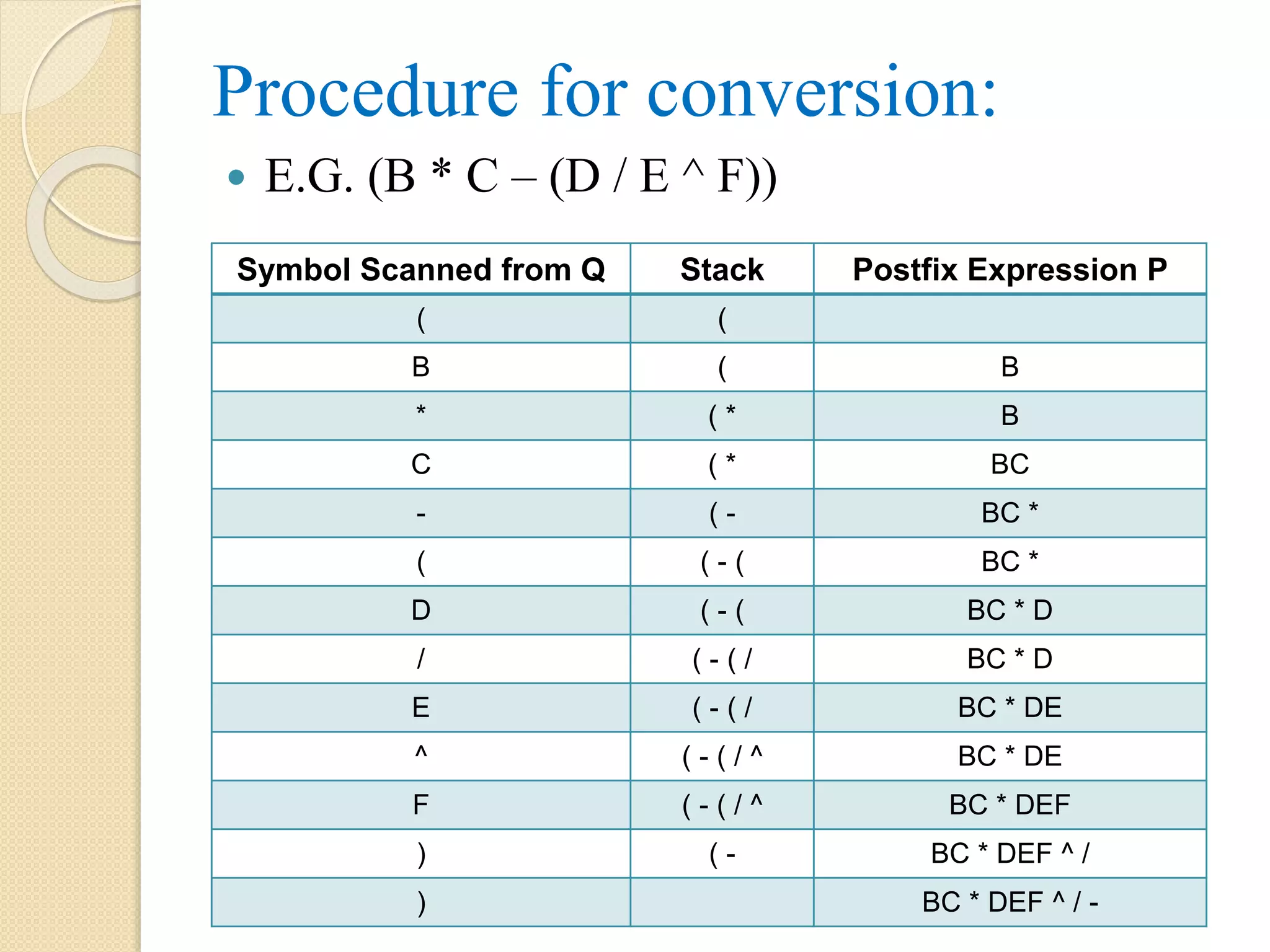
![Postfix Expression Evaluation using Stack: [Assume ‘P’ is a postfix expression] Step 1: Add ‘)’ at the end of P. Step 2: Repeatedly scan ‘P’ from left to right until ‘)’ encountered. Step 2.1: if P[I] is an operand, then push the operand onto stack. Step 2.2: else if P[I] is an operator x then Step 2.2.1: pop two elements from stack (1st element is A and 2nd is B). Step 2.2.2: Evaluate B x A Step 2.2.3: push result back to stack [End of if] [End of step 2] Step 3: Value = Stack[TOP] Step 4: Display Value Step 5: Exit](https://image.slidesharecdn.com/datastructureusingcmodule1-170525065731/75/Data-structure-using-c-module-1-66-2048.jpg)
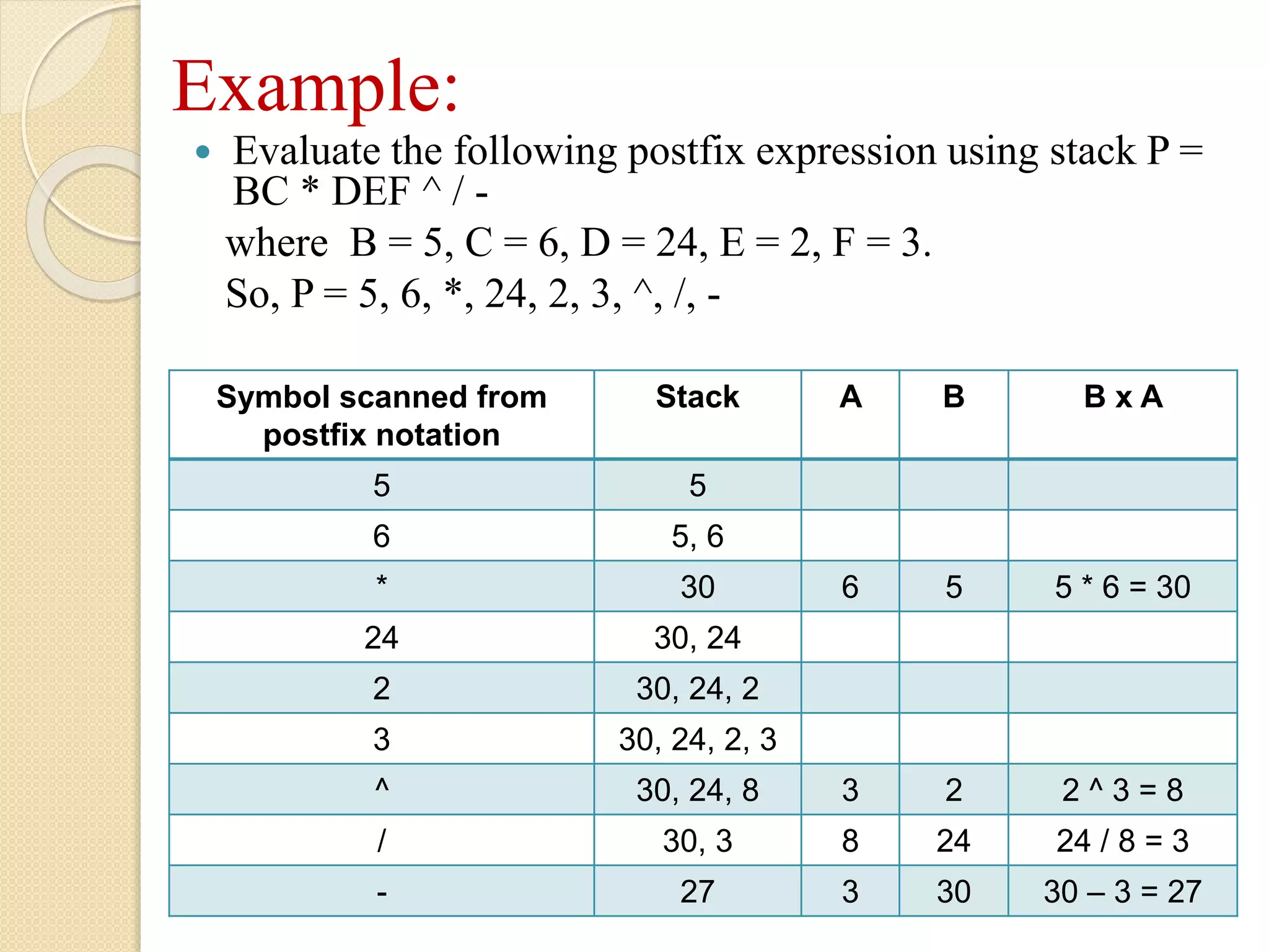
![Infix to Prefix Conversion using Stack: [Assume Q is an infix expression and there are two stacks S1 and S2 exist.] • Step 1: Add left parenthesis ‘(‘ at the beginning of the expression. • Step 2: PUSH ‘)’ onto stack S1. • Step 3: Repeatedly scan Q in right to left order, until Stack S1 is empty. Step 3.1: if Q[I] is an operand, then push it into stack S2. Step 3.2: else if Q[I] is ‘)‘, then push it into stack S1. Step 3.3: else if Q[I] is an operator(op) then,](https://image.slidesharecdn.com/datastructureusingcmodule1-170525065731/75/Data-structure-using-c-module-1-68-2048.jpg)
![Step 3.3.1: Set x = POP(S1) Step 3.3.2: Repeat while x is an operator AND (Precedence (x) > Precedence (op)) PUSH (x) onto stack S2. Set x = POP (S1) [End of while – step 3.3.2] Step 3.3.3. PUSH (x) onto stack S1 Step 3.3.4: PUSH (op) onto stack S1 Step 3.4: else if Q[I] is ‘(‘, then Step 3.4.1: Set x = POP (S1) Step 3.4.2: Repeat, while (x != ‘)’) [until right parenthesis found] Step 3.4.2.1: PUSH (x) onto stack S2 Step 3.4.2.2: Set x = POP (S1)](https://image.slidesharecdn.com/datastructureusingcmodule1-170525065731/75/Data-structure-using-c-module-1-69-2048.jpg)
![[End of while – step 3.4.2] [End of if – Step – 3.1] [End of loop – Step – 3] • Step 4: Repeat, while stack S2 is not empty. Step 4.1: Set x = POP (S2) Step 4.2: Display x [End of While] • Step 5: Exit](https://image.slidesharecdn.com/datastructureusingcmodule1-170525065731/75/Data-structure-using-c-module-1-70-2048.jpg)
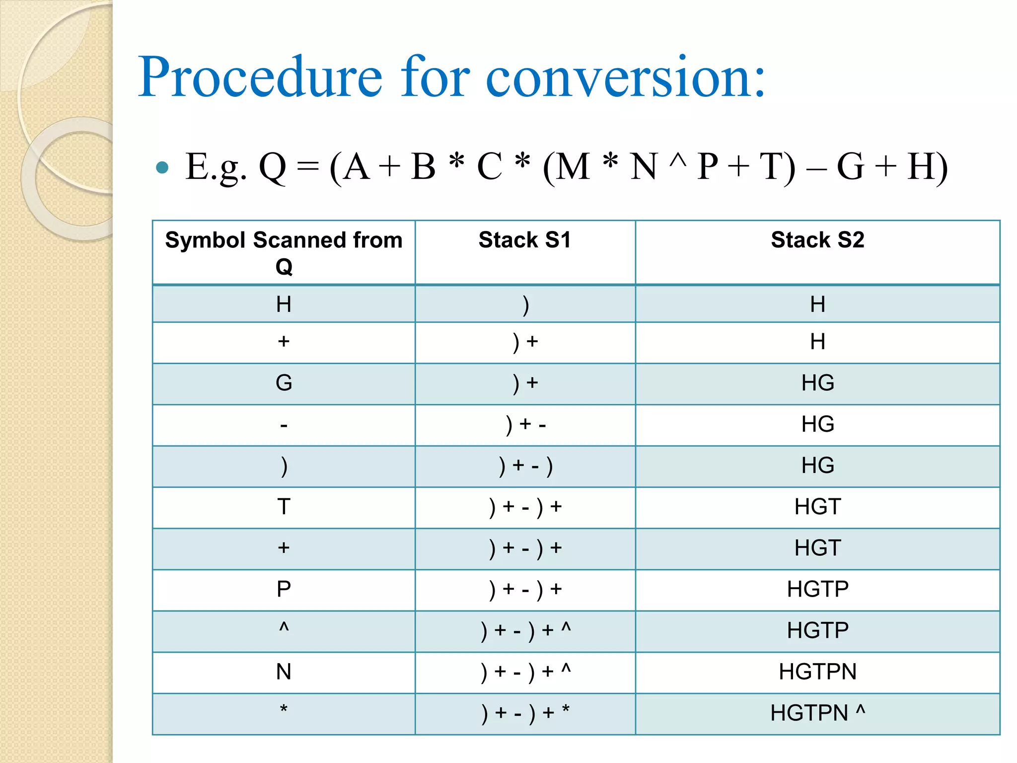
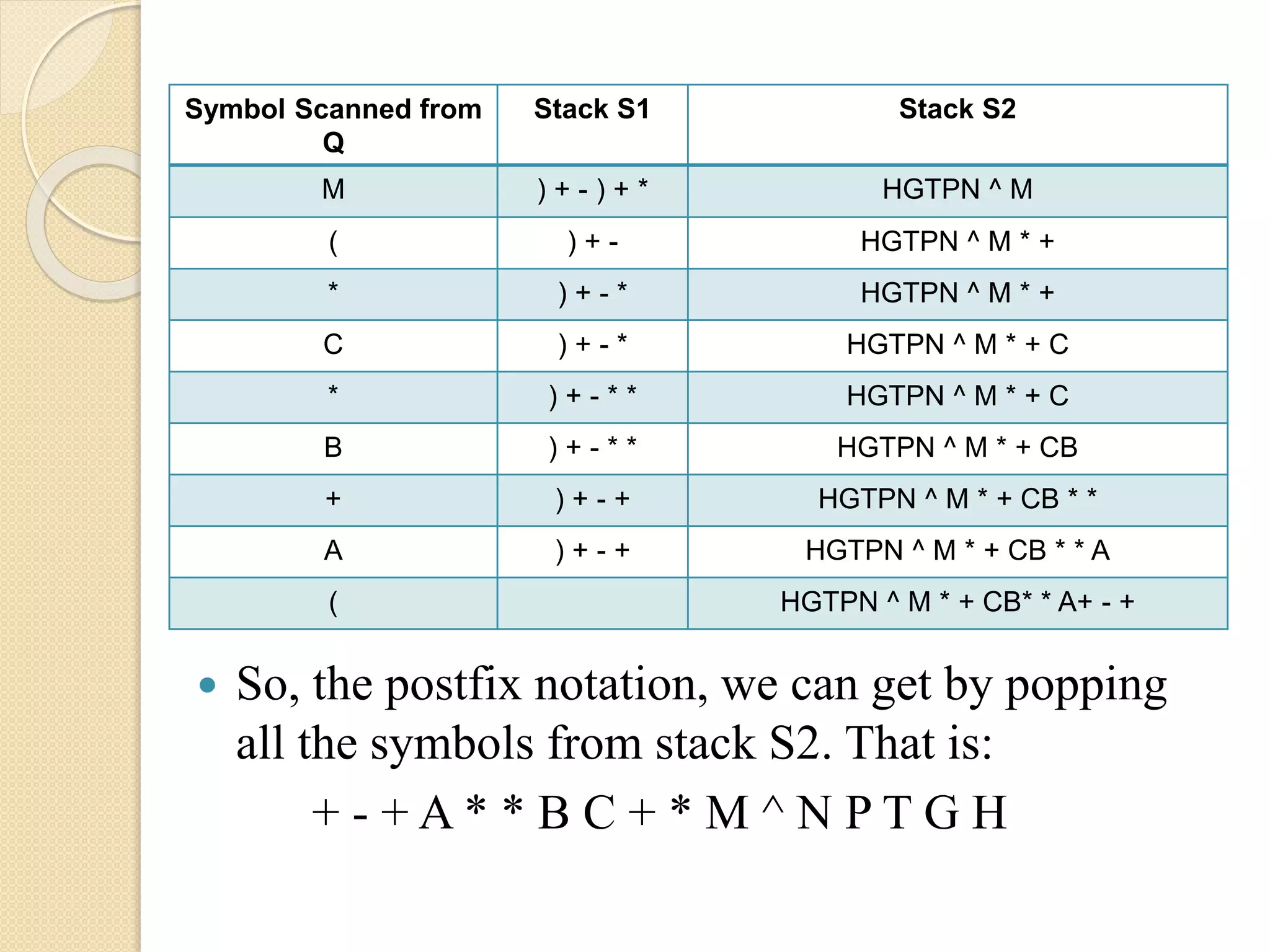
![Prefix Expression Evaluation using Stack: [Assume ‘P’ is a prefix expression] Step 1: Add ‘(’ at the beginning of prefix expression. Step 2: Repeatedly scan from ‘P’ in right to left order until ‘(’ encountered. Step 2.1: if P[I] is an operand, then push the operand onto stack. Step 2.2: else if P[I] is an operator (op) then Step 2.2.1: pop two elements from stack (1st element is A and 2nd is B). Step 2.2.2: Evaluate A (op) B Step 2.2.3: push result back to stack [End of if] [End of step 2] Step 3: Value = Stack[TOP] Step 4: Display Value Step 5: Exit](https://image.slidesharecdn.com/datastructureusingcmodule1-170525065731/75/Data-structure-using-c-module-1-73-2048.jpg)
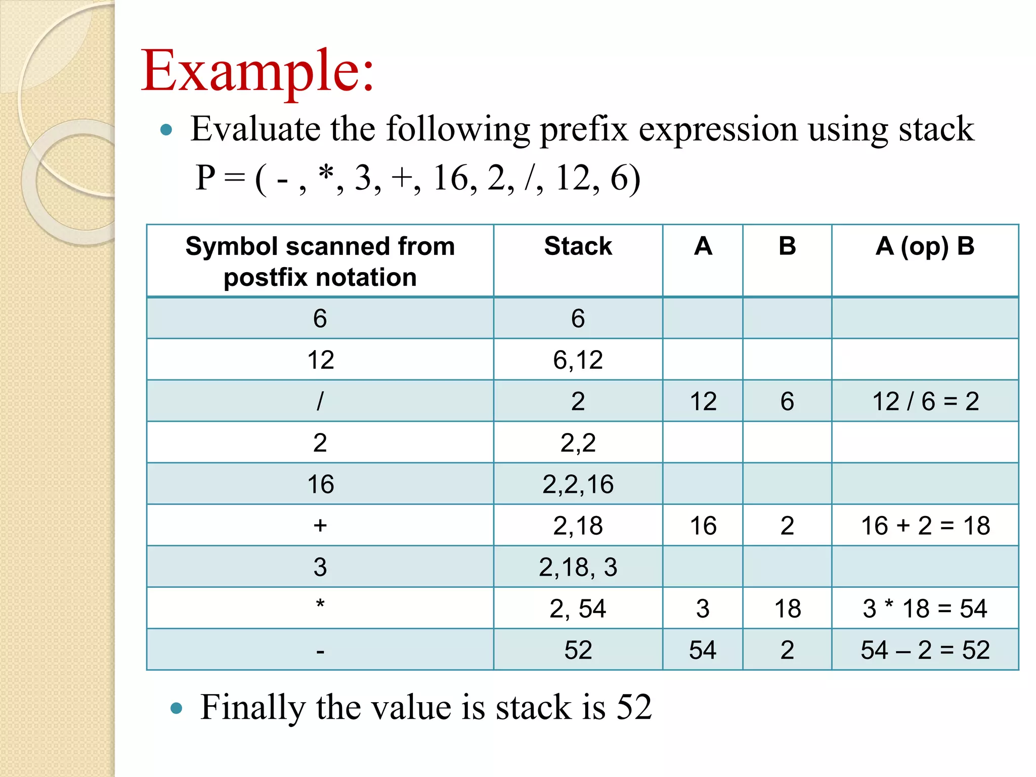
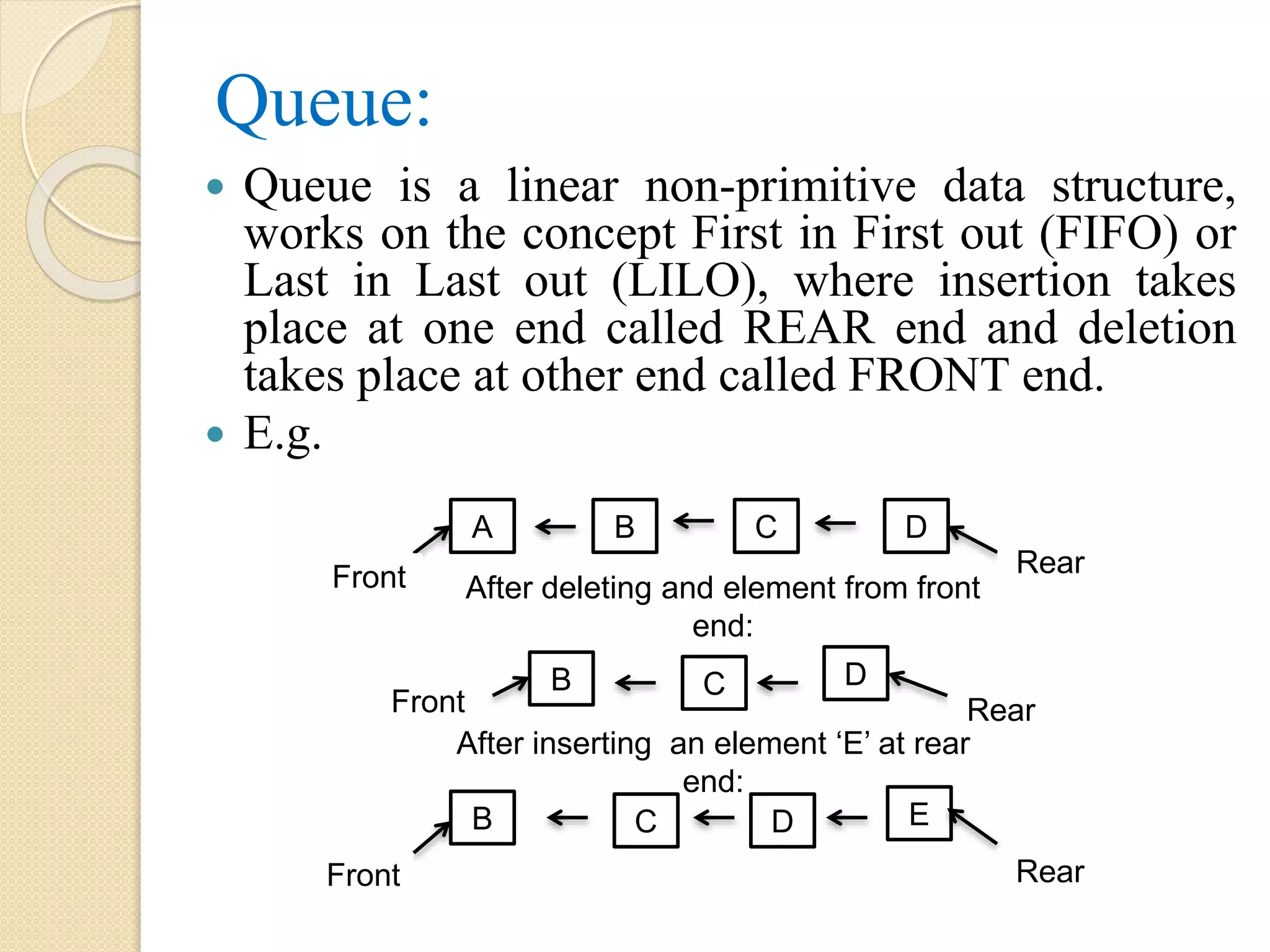
![Example: Let Q[MAXSIZE] is an array that represents a queue in the memory and at the beginning, it is empty and MAXSIZE = 10. That is: Front = Rear = NULL or -1. 0 1 2 3 4 5 6 7 8 9 A B C D C D C D E F G 0 1 2 3 4 5 6 7 8 9 0 1 2 3 4 5 6 7 8 9 Insert 4 elements A, B, C, D Delete 2 elements Insert 3 elements E, F, G 0 1 2 3 4 5 6 7 8 9 F = 2, R = 6 F = 2, R = 3 F = 0, R = 3 F = -1, R = -1 MAXSIZE - 1](https://image.slidesharecdn.com/datastructureusingcmodule1-170525065731/75/Data-structure-using-c-module-1-79-2048.jpg)
![Linear Queue Insertion Algorithm: Qinsert(Queue[MAXSIZE], ITEM) Step 1: if Rear = MAXSIZE – 1, then Display “Overflow or Queue is Full” Exit Step 2: else if Front = -1 or Rear = -1, then Front = 0 Rear = 0 Step 3: else Rear = Rear + 1 [End of if] Step 4: Queue[Rear] = ITEM Step 5: Exit](https://image.slidesharecdn.com/datastructureusingcmodule1-170525065731/75/Data-structure-using-c-module-1-82-2048.jpg)
![Linear Queue Deletion Algorithm: Qdelete (Queue[MAXSIZE]) Step 1: Let ITEM Step 2: if Front = -1 or Rear = -1, then Display “Underflow or Queue empty” Exit [End of if] Step 3: ITEM = Queue[Front] Step 4: Display “deleted item is”, ITEM Step 5: else if Front = Rear, then Front = -1 Rear = -1 Step 6: else Front = Front + 1 Step 7: Exit](https://image.slidesharecdn.com/datastructureusingcmodule1-170525065731/75/Data-structure-using-c-module-1-83-2048.jpg)
![Circular Queue: It is a queue of circular nature, in which it is possible to insert a new element at the first location, when the last location of the queue is occupied. In other words, if an Q[MAXSIZE] represents a circular queue then after inserting an element at (MAXSIZE -1)th location of the array, the next element will be inserted at the very first location at index 0.](https://image.slidesharecdn.com/datastructureusingcmodule1-170525065731/75/Data-structure-using-c-module-1-84-2048.jpg)
![Circular Queue Representation: E.g. Let an array A[5] is maintained in form of circular queue. Here overflow situation arises only when Rear is before the Front position. 10 A[0] A[1] A[2] A[3] A[4] 20 30 Front Rear](https://image.slidesharecdn.com/datastructureusingcmodule1-170525065731/75/Data-structure-using-c-module-1-86-2048.jpg)
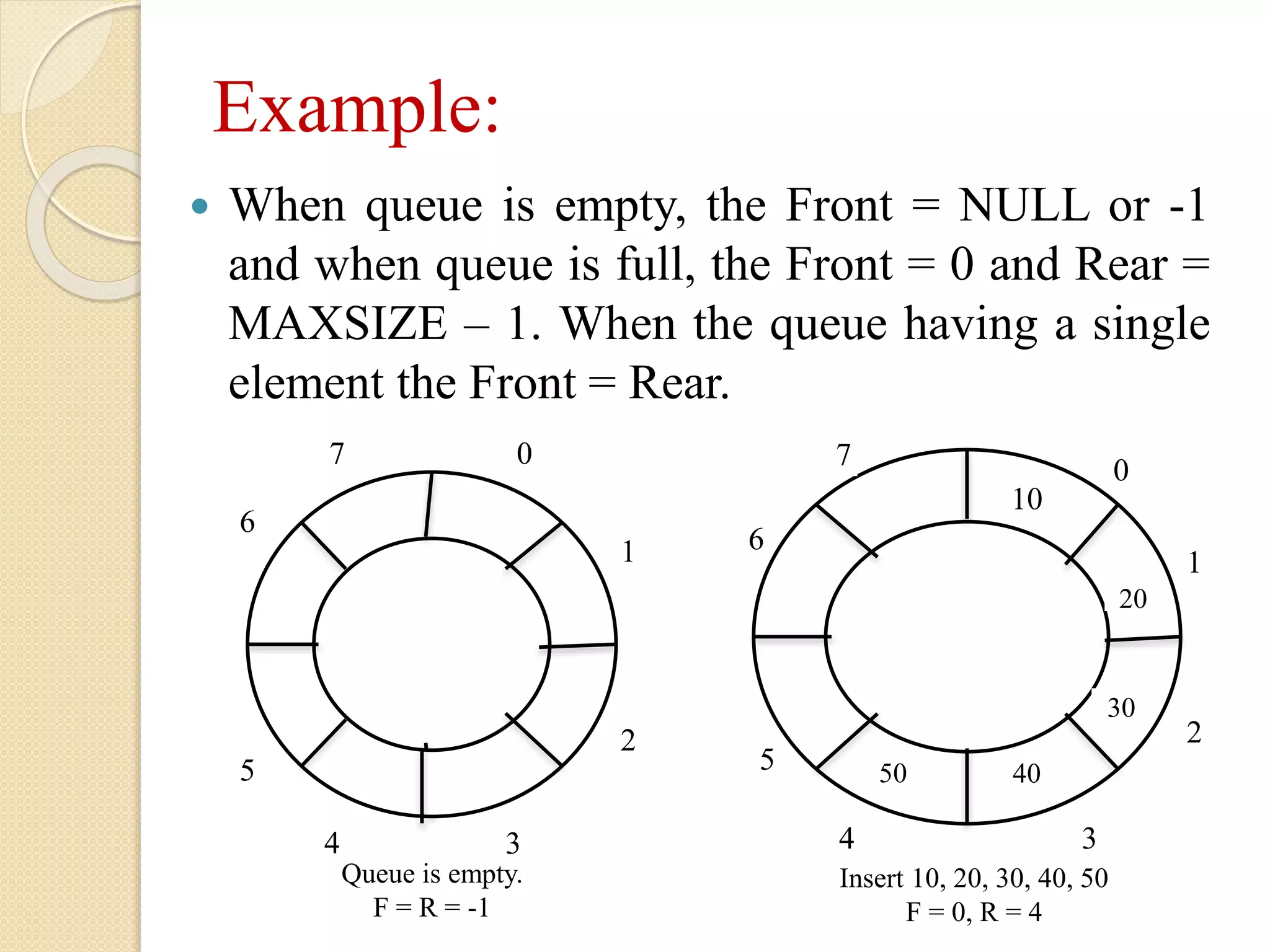
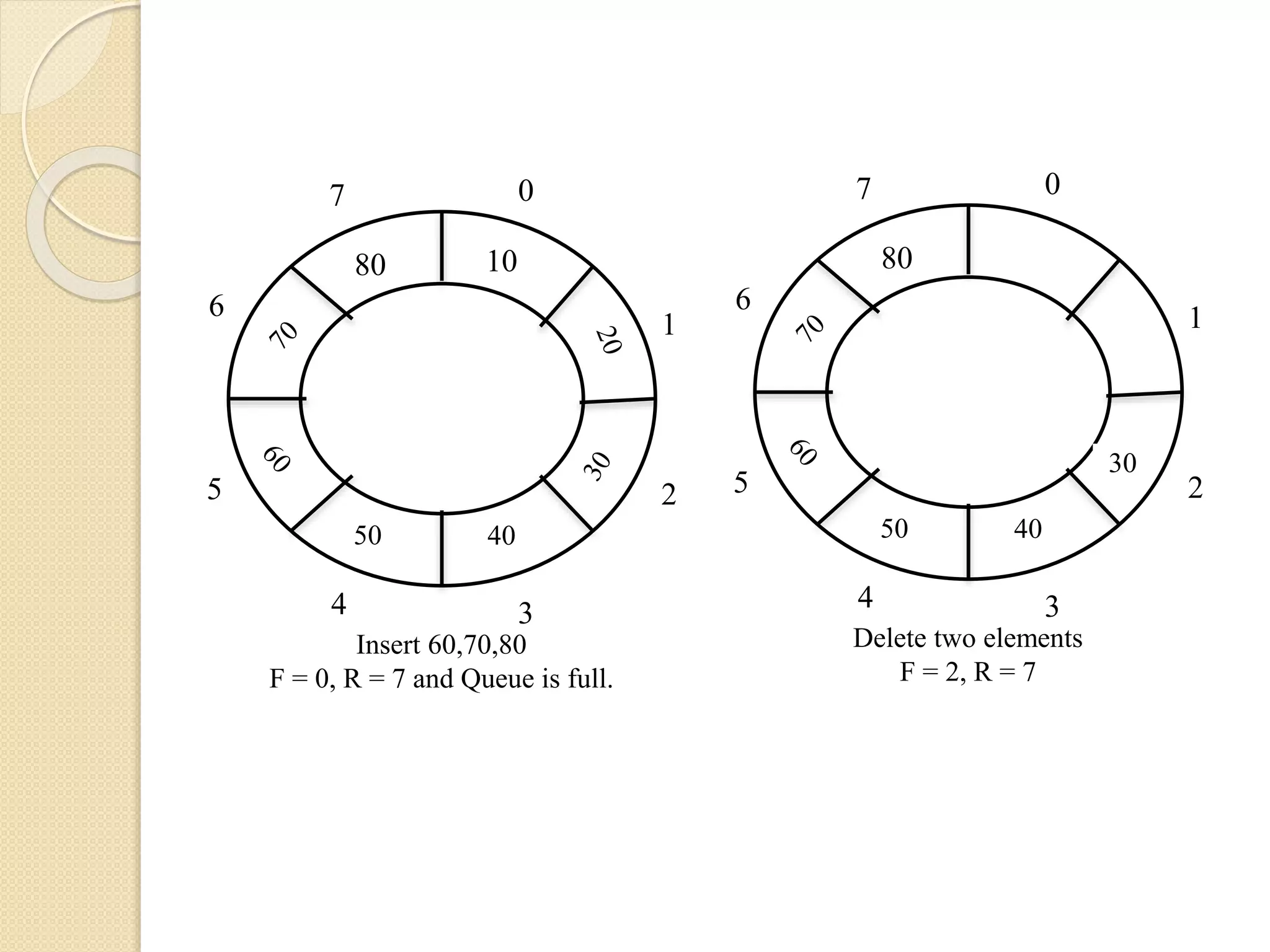
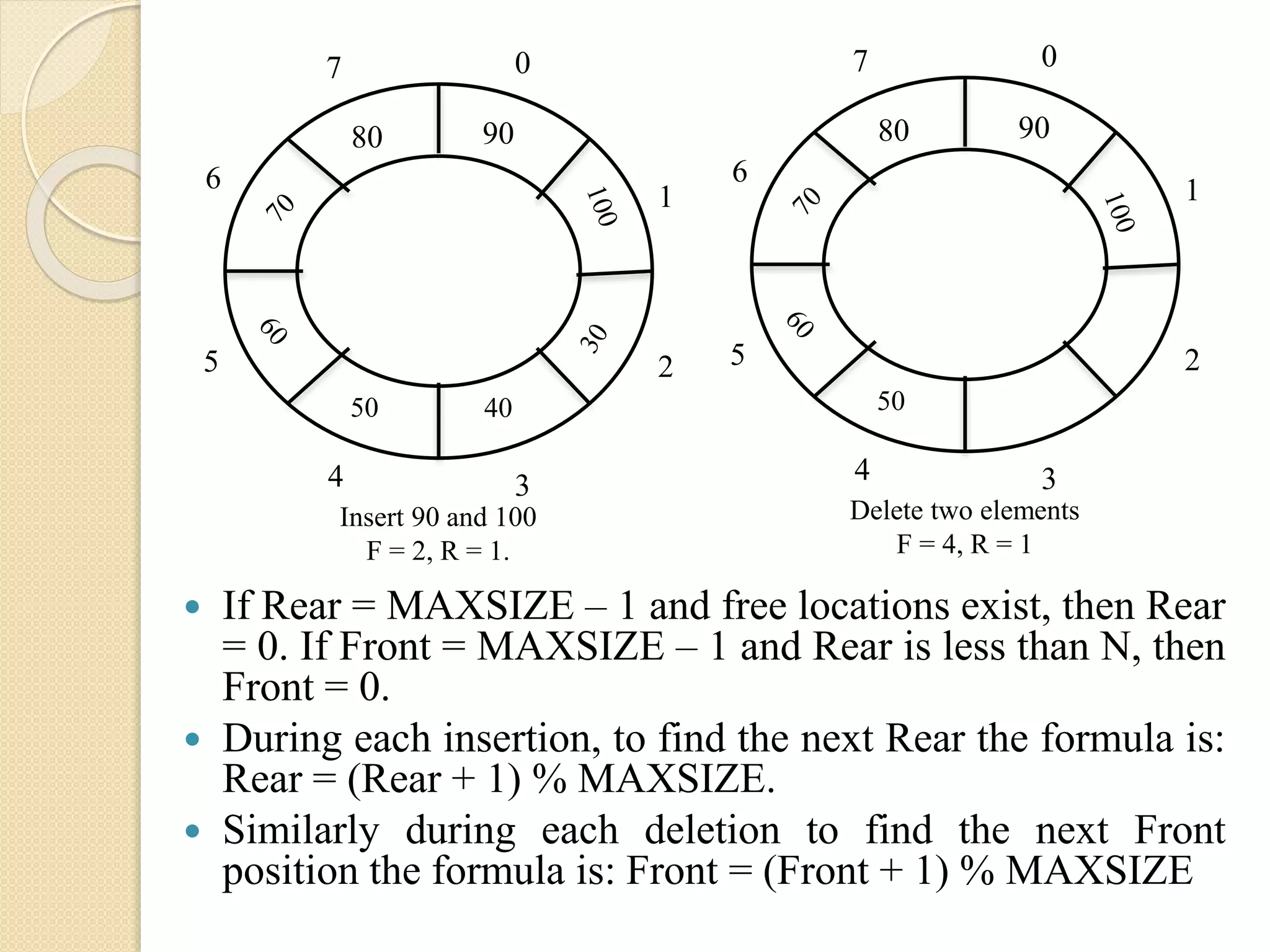
![Insertion in a Circular Queue: CQinsert(Queue[MAXSIZE], ITEM) Step 1: if (Front = 0 AND Rear = MAXSIZE – 1) OR (Front = (Rear + 1) % MAXSIZE), then Display “Overflow” Exit Step 2: else if Front = -1 or Rear = -1 then Front = 0 Rear = 0 Step 3: else Rear = (Rear + 1) % MAXSIZE [End of if] Step 4: Queue[Rear] = ITEM Step 5: Exit](https://image.slidesharecdn.com/datastructureusingcmodule1-170525065731/75/Data-structure-using-c-module-1-90-2048.jpg)
![Deletion in a Circular Queue: CQdelete(Queue, Front, Rear) Step 1: Let ITEM Step 2: if Front = -1 or Rear = -1 then Display “Queue is empty or Underflow” Exit [End of if] Step 3: ITEM = Queue[Front] Step 4: Display “deleted item is”, ITEM Step 5: if Front = Rear, then Front = -1 Rear = -1 Step 6: else Front = (Front + 1) % MAXSIZE [End of if] Step 7: Exit](https://image.slidesharecdn.com/datastructureusingcmodule1-170525065731/75/Data-structure-using-c-module-1-91-2048.jpg)
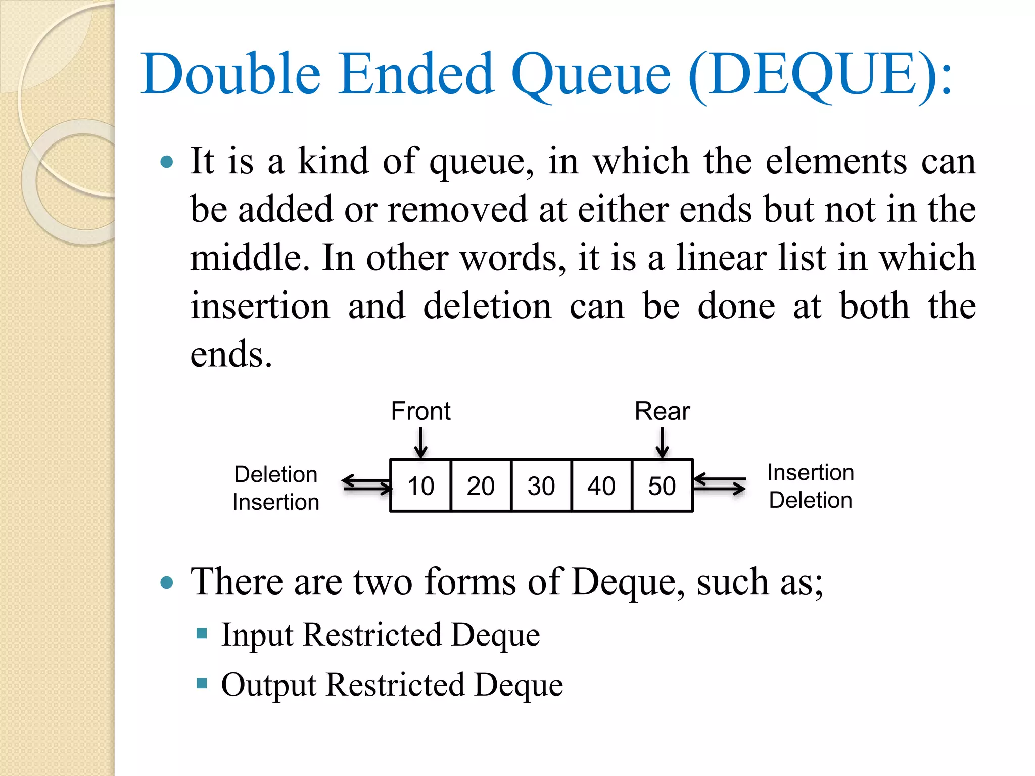
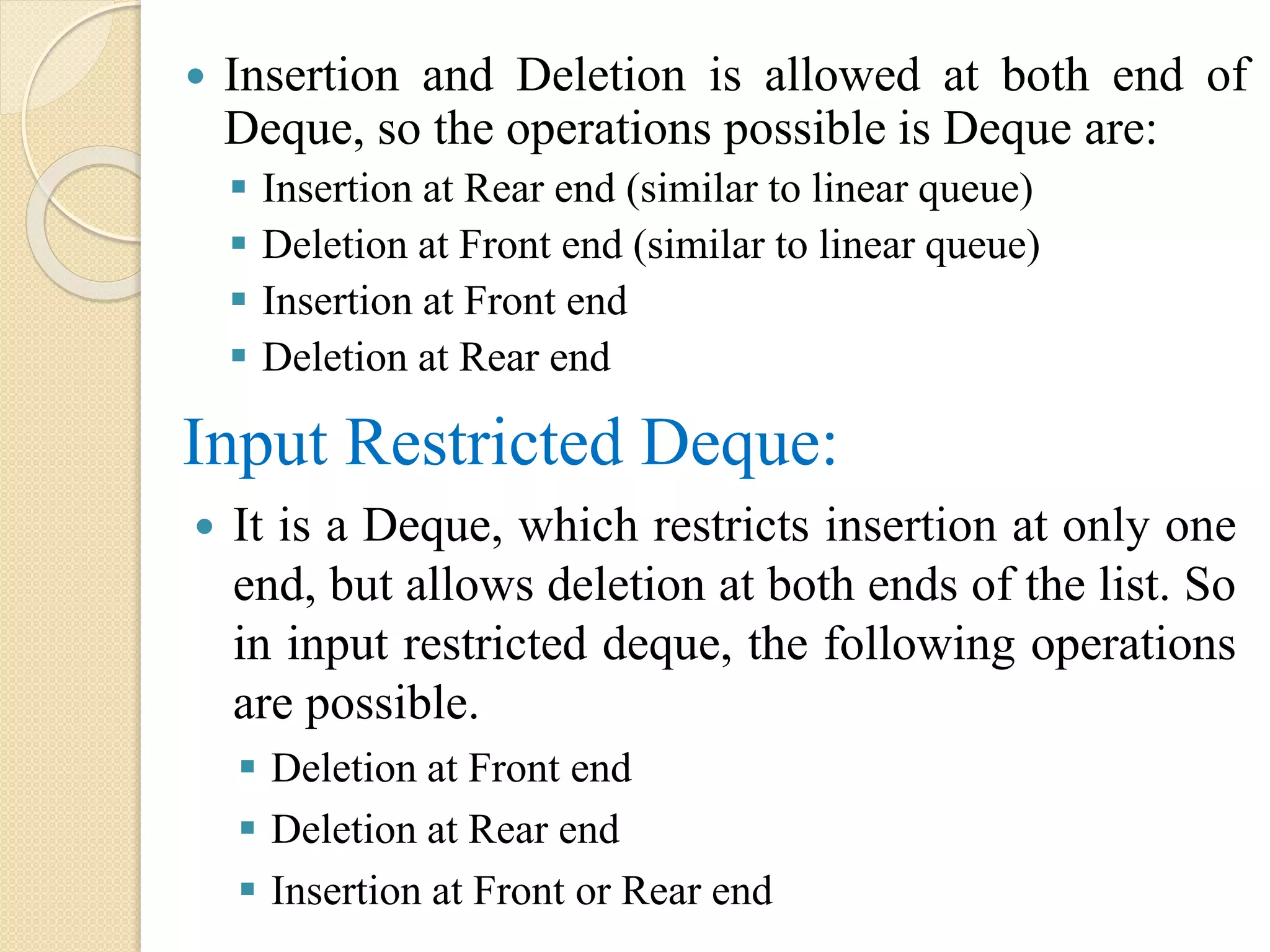
![C-Function for insertion at rear end of Deque: void dqinsert_Rear (int Q[ ], int ITEM) { if(rear == MAXSIZE – 1) { printf(“Deque is full”); } else { Rear = Rear + 1; Q[Rear] = ITEM; } }](https://image.slidesharecdn.com/datastructureusingcmodule1-170525065731/75/Data-structure-using-c-module-1-95-2048.jpg)
![C-Function for insertion at front end of Deque: void dqinsert_Front (int Q[ ], int Front, int Rear, int ITEM, int MAXSIZE) { if(Front == 0) { printf(“Deque is full”); } else { Front = Front - 1; Q[Front] = ITEM; } }](https://image.slidesharecdn.com/datastructureusingcmodule1-170525065731/75/Data-structure-using-c-module-1-96-2048.jpg)
![C-Function for deletion at front end of Deque: void dqdelete_Front (int Q[ ]) { int ITEM; if (Front == -1) { printf(“Deque is empty”); } else if (Front == Rear) { ITEM = Q[Front]; Front = Rear = - 1; printf(“deleted item is %d”, ITEM); } }](https://image.slidesharecdn.com/datastructureusingcmodule1-170525065731/75/Data-structure-using-c-module-1-97-2048.jpg)
![C-Function for deletion at rear end of Deque: void dqdelete_Rear (int Q[ ]) { int ITEM; if (Front == -1 || Rear == -1) { printf(“Deque is empty”); exit(0); } ITEM = Q[Rear]; if (Front == Rear) { Front = Rear = - 1; } else { Rear = Rear – 1; } printf(“deleted item is %d”, ITEM); } }](https://image.slidesharecdn.com/datastructureusingcmodule1-170525065731/75/Data-structure-using-c-module-1-98-2048.jpg)

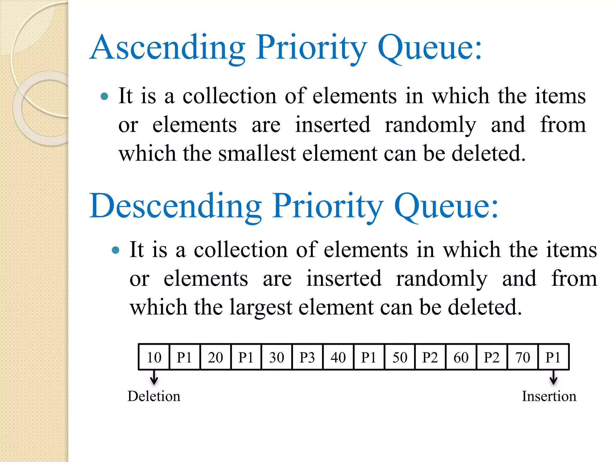
![Linked List: Linked list is a linear collection of data elements called nodes, each of which is a memory location that contains two parts. That is: ◦ Information of element or data ◦ Link field contains the address of next node or points to the next element stored in the list. INFO LINK Node XSTART [Structure of a node in linked list]](https://image.slidesharecdn.com/datastructureusingcmodule1-170525065731/75/Data-structure-using-c-module-1-101-2048.jpg)
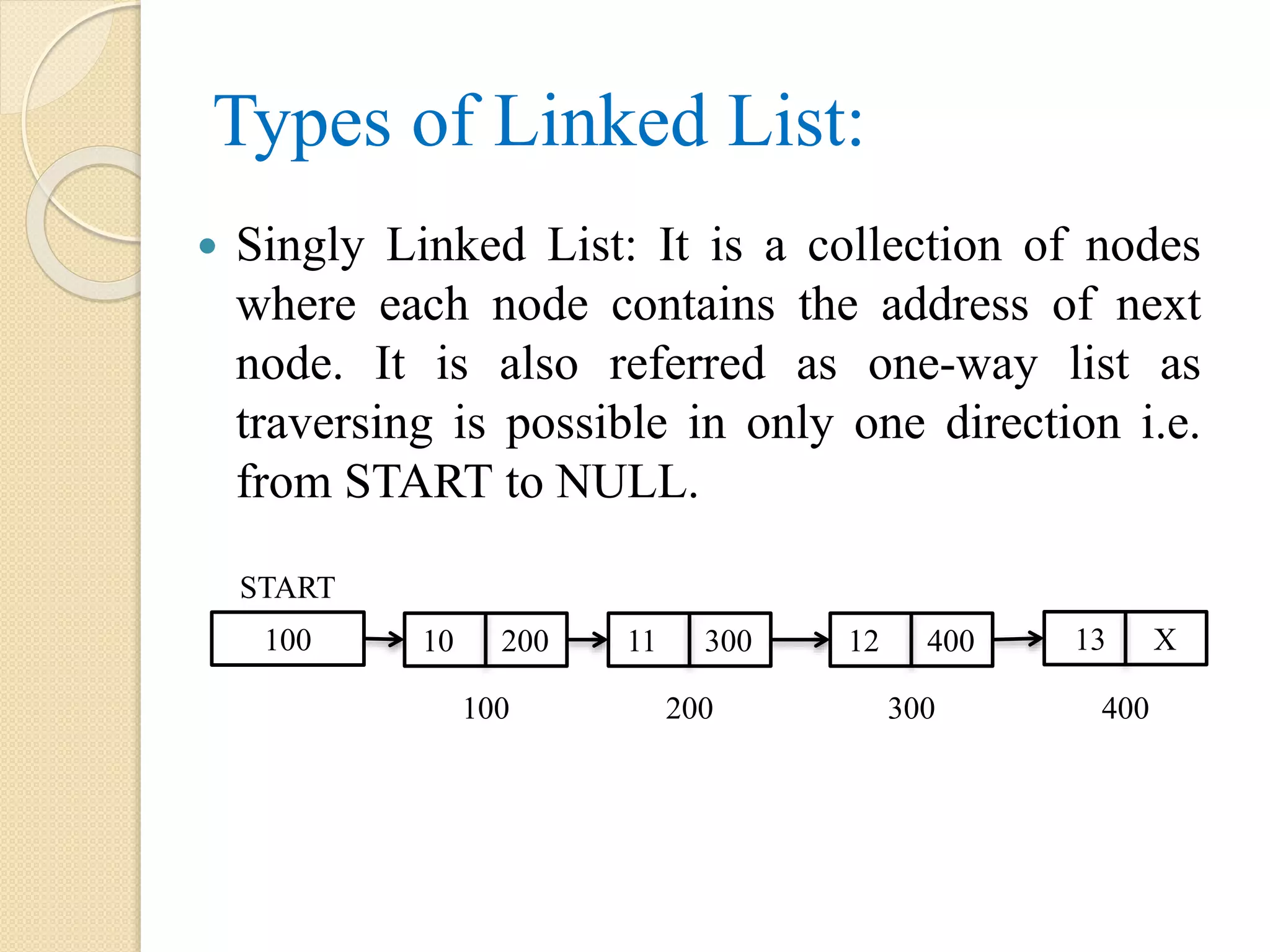
![Psuedo code: Step 1: if AVAIL = NULL, then Display “ Insufficient Memory or Overflow” Exit Step 2: else FRESH = AVAIL AVAIL = LINK[AVAIL] INFO[FRESH] = ITEM LINK[FRESH] = NULL [End of if] 200 200 AVAIL 100 300 400 X 200 300 400 100 FRESH Note: the dotted arrow represents the link which exist before the operations](https://image.slidesharecdn.com/datastructureusingcmodule1-170525065731/75/Data-structure-using-c-module-1-110-2048.jpg)
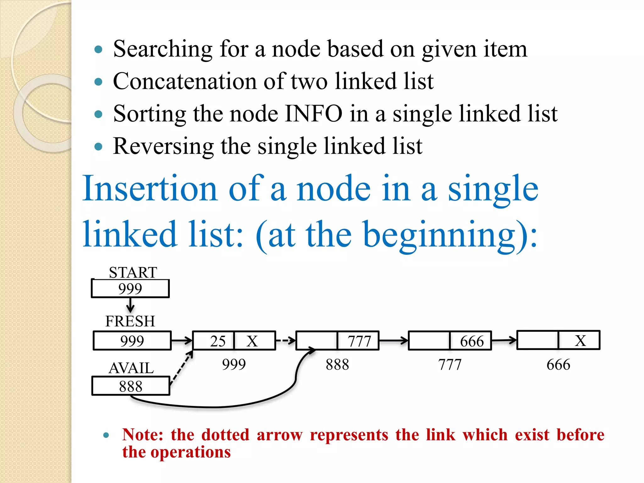
![Algorithm: Creation(AVAIL, INFO, LINK, START, FRESH, ITEM) Step 1: if AVAIL = NULL, then Display “Insufficient Memory or Overflow” Exit Step 2: else FRESH = AVAIL AVAIL = LINK[AVAIL] INFO[FRESH] = ITEM LINK[FRESH] = NULL START = FRESH [End of if] Step 3: Exit](https://image.slidesharecdn.com/datastructureusingcmodule1-170525065731/75/Data-structure-using-c-module-1-113-2048.jpg)
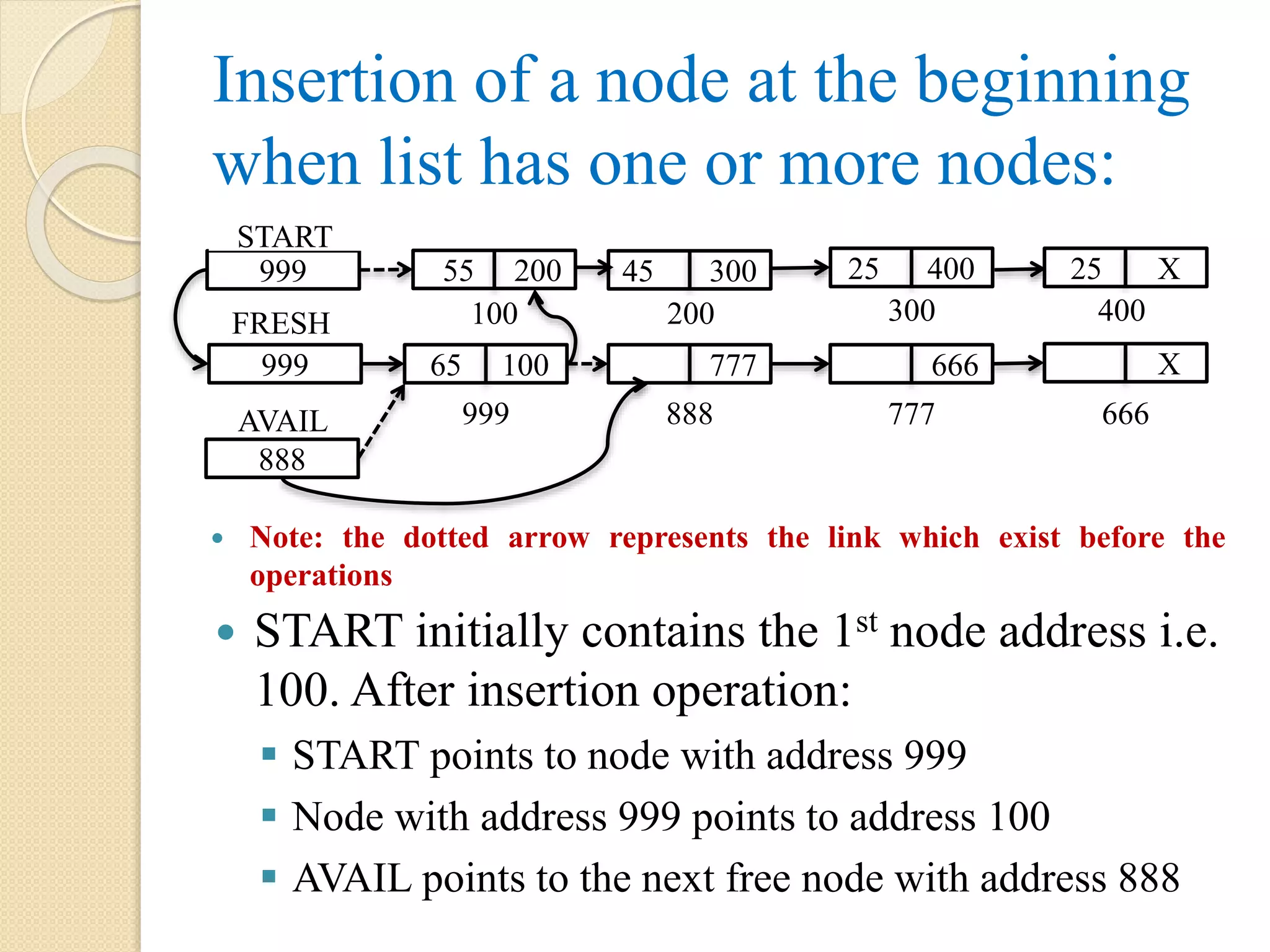
![Algorithm: Insert_First(INFO, LINK, START, AVAIL, ITEM) Step 1: if AVAIL = NULL, then Display “Insufficient Memory or Overflow” Exit [End of if] Step 2: if START = NULL, then START = FRESH Step 3: else FRESH = AVAIL AVAIL = LINK[AVAIL] INFO[FRESH] = ITEM LINK[FRESH] = START START = FRESH [End of if] Step 4: Exit](https://image.slidesharecdn.com/datastructureusingcmodule1-170525065731/75/Data-structure-using-c-module-1-115-2048.jpg)
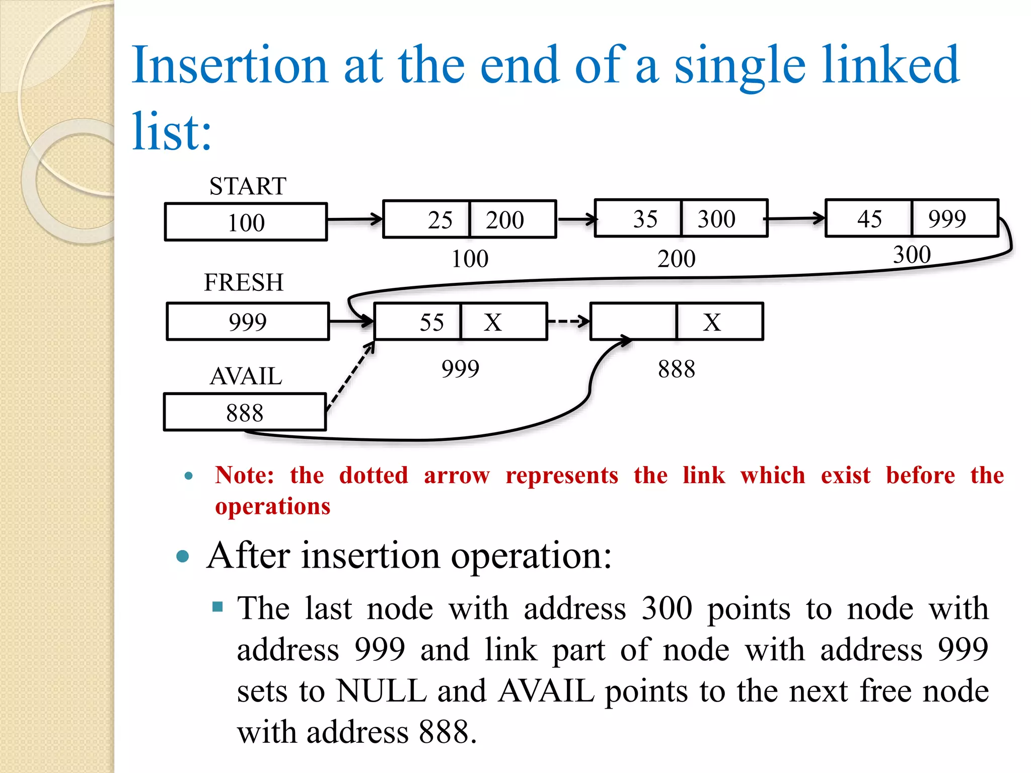
![Algorithm: Insert_End (INFO, LINK, START, AVAIL, ITEM) Step 1: Let PTR Step 2: if AVAIL = NULL, then Display “Insufficient Memory or Overflow” Exit Step 3: else FRESH = AVAIL AVAIL = LINK[AVAIL] INFO[FRESH] = ITEM LINK[FRESH] = NULL [End of if] Step 3.1: if START = NULL, then START = FRESH](https://image.slidesharecdn.com/datastructureusingcmodule1-170525065731/75/Data-structure-using-c-module-1-117-2048.jpg)
![ Step 3.2: else PTR = START Repeat while LINK[PTR] != NULL PTR = LINK[PTR] [End of while] LINK[PTR] = FRESH [End of Step 3.1] [End of Step 2] Step 4: Exit](https://image.slidesharecdn.com/datastructureusingcmodule1-170525065731/75/Data-structure-using-c-module-1-118-2048.jpg)
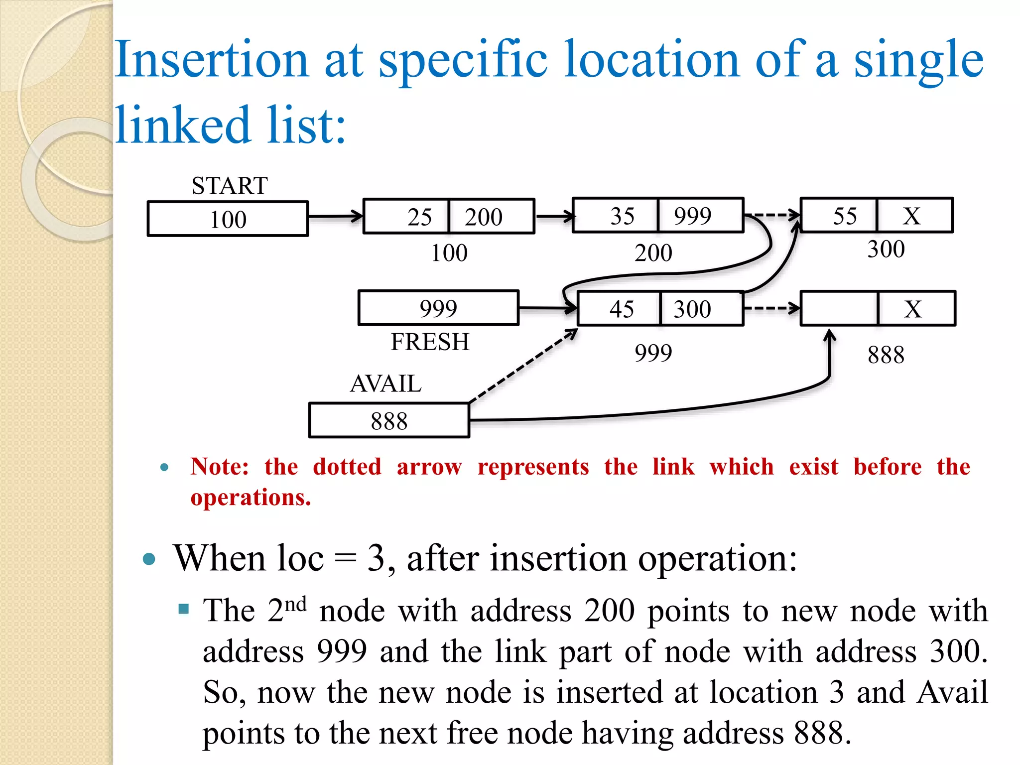
![Algorithm: Insert_Loc(INFO, LINK, START, AVAIL, LOC, ITEM, PTR, PREV) Step 1: Let I = 1 Step 2: if AVAIL = NULL, then Display “Insufficient Memory or Overflow” Exit Step 3: else FRESH = AVAIL AVAIL = LINK[AVAIL] INFO[FRESH] = ITEM LINK[FRESH] = NULL Step 3.1: if START = NULL, then Display “List doesn’t exist”. Step 3.2: else](https://image.slidesharecdn.com/datastructureusingcmodule1-170525065731/75/Data-structure-using-c-module-1-120-2048.jpg)
![ Step 3.2.1: PTR = START Step 3.2.2: Repeat, while I < LOC AND PTR != NULL PREV = PTR PTR = LINK[PTR] I = I + 1 [End of while] Step 3.2.3: if PTR = NULL, then Display “Location not found”. Step 3.2.4: else if PTR = START, then LINK[FRESH] = START START = FRESH Step 3.2.5: else LINK[PREV] = FRESH LINK[FRESH] = PTR [End of if – step 3.2.3] [End of step 3.1] [End of step 2] Step 4: Exit](https://image.slidesharecdn.com/datastructureusingcmodule1-170525065731/75/Data-structure-using-c-module-1-121-2048.jpg)
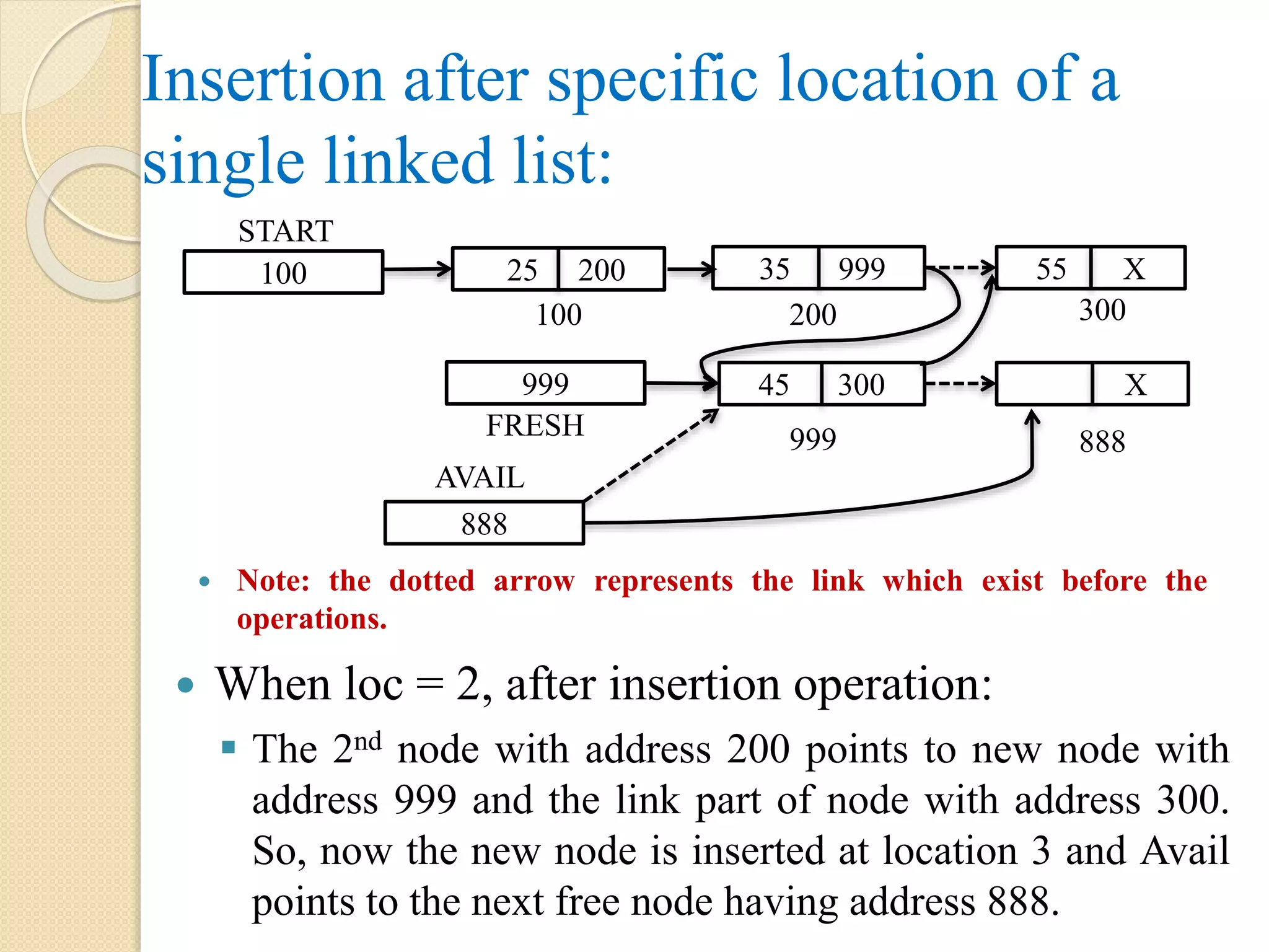
![Algorithm: InsertAfter_Loc(INFO, LINK, START, AVAIL, LOC, ITEM, PTR) Step 1: Let I Step 2: if AVAIL = NULL, then Display “Insufficient Memory or Overflow” Exit Step 3: else FRESH = AVAIL AVAIL = LINK[AVAIL] INFO[FRESH] = ITEM LINK[FRESH] = NULL Step 3.1: if START = NULL, then Display “List doesn’t exist”. Step 3.2: else](https://image.slidesharecdn.com/datastructureusingcmodule1-170525065731/75/Data-structure-using-c-module-1-123-2048.jpg)
![ Step 3.2.1: PTR = START Step 3.2.2: Repeat, for I = 1 to LOC – 1 increasing by 1 PTR = LINK[PTR] [End of for] Step 3.2.3: if PTR = NULL, then Display “Invalid entry for location”. Step 3.2.4: else LINK[FRESH] = LINK[PTR] LINK[PTR] = FRESH [End of if – step 3.2.3] [End of step 3.1] [End of step 2] Step 4: Exit](https://image.slidesharecdn.com/datastructureusingcmodule1-170525065731/75/Data-structure-using-c-module-1-124-2048.jpg)
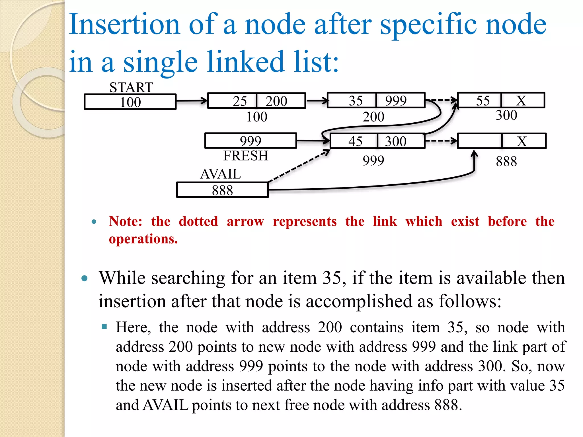
![Algorithm: InsertAfterNode(INFO, LINK, START, AVAIL, NEWITEM, ITEM, PTR) Step 1: START Step 2: if AVAIL = NULL, then Display “Insufficient Memory or Overflow” Exit Step 3: else FRESH = AVAIL AVAIL = LINK[AVAIL] INFO[FRESH] = NEWITEM LINK[FRESH] = NULL Step 3.1: if START = NULL, then Display “List doesn’t exist”. Step 3.2: else](https://image.slidesharecdn.com/datastructureusingcmodule1-170525065731/75/Data-structure-using-c-module-1-126-2048.jpg)
![ Step 3.2.1: PTR = START Step 3.2.2: Repeat, while PTR != NULL AND ITEM != INFO[PTR] PTR = LINK[PTR] [End of while] Step 3.2.3: if PTR = NULL, then Display “Item does not exist”. Step 3.2.4: else LINK[FRESH] = LINK[PTR] LINK[PTR] = FRESH [End of step 3.1] [End of step 2] Step 4: Exit](https://image.slidesharecdn.com/datastructureusingcmodule1-170525065731/75/Data-structure-using-c-module-1-127-2048.jpg)
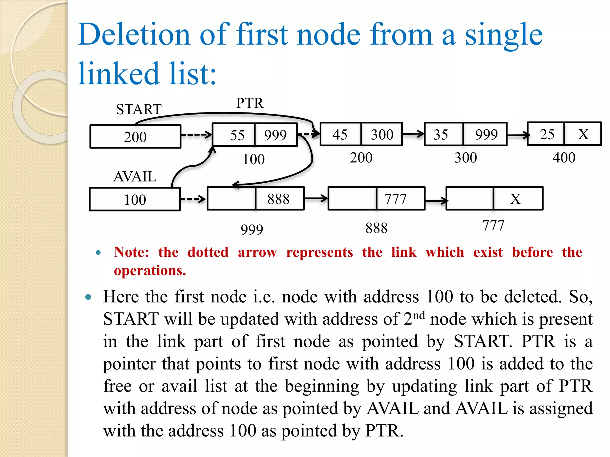
![Algorithm: Deletion_First(INFO, LINK, START, AVAIL, PTR) Step 1: if START = NULL, then Display “List does not exist or Underflow”. Step 2: else PTR = START START = LINK[PTR] LINK[PTR] = AVAIL AVAIL = PTR [End of if] Step 3: exit](https://image.slidesharecdn.com/datastructureusingcmodule1-170525065731/75/Data-structure-using-c-module-1-129-2048.jpg)
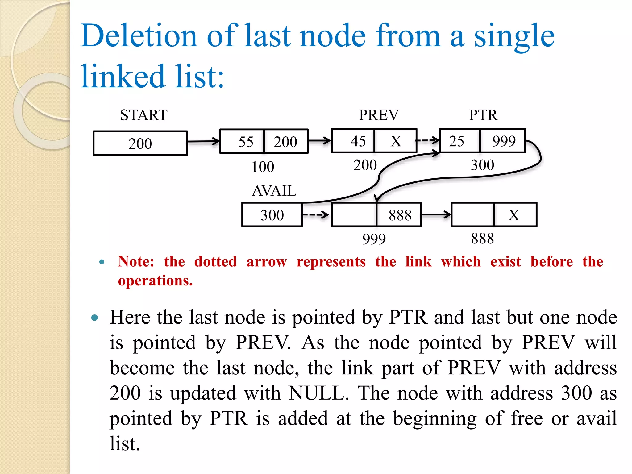
![Algorithm: Deletion_End(START, LINK, INFO, PTR, PREV, AVAIL) Step 1: if START = NULL, then Display “List is empty”. Step 2: else Step 2.1: PTR = START Step 2.2: Repeat while LINK[PTR] != NULL PREV = PTR PTR = LINK[PTR] [End of while] Step 2.3: LINK[PREV] = NULL Step 2.4: LINK[PTR] = AVAIL Step 2.5: AVAIL = PTR [End of if] Step 3: exit](https://image.slidesharecdn.com/datastructureusingcmodule1-170525065731/75/Data-structure-using-c-module-1-131-2048.jpg)
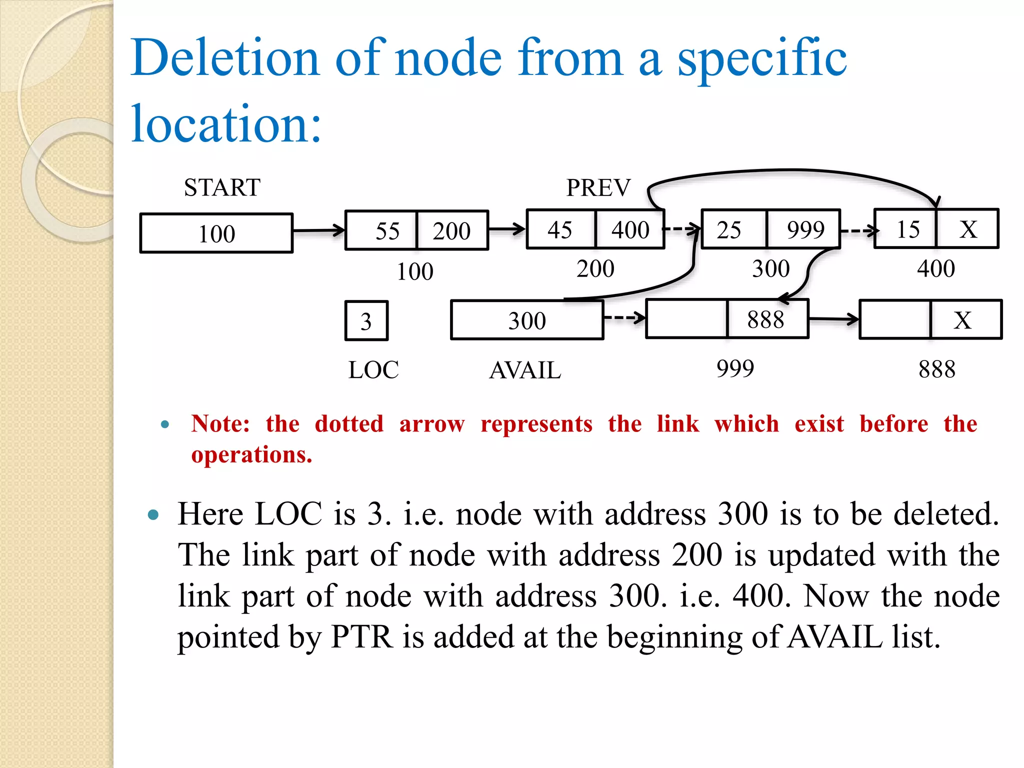
![Algorithm: Deletion_LOC(START, LINK, INFO, PTR, PREV, LOC) Step 1: Let I = 1 Step 2: PTR = START Step 3: Repeat while I < LOC AND PTR != NULL PREV = PTR PTR = LINK[PTR] I = I + 1 [End of while] Step 4: if PTR = NULL, then display “Location doesn’t exist”. Step 5: else if PTR = START, then START = LINK[PTR] Step 6: else LINK[PREV] = LINK[PTR] [End of if] Step 7: LINK[PTR] = AVAIL Step 8: AVAIL = PTR Step 9: exit](https://image.slidesharecdn.com/datastructureusingcmodule1-170525065731/75/Data-structure-using-c-module-1-133-2048.jpg)
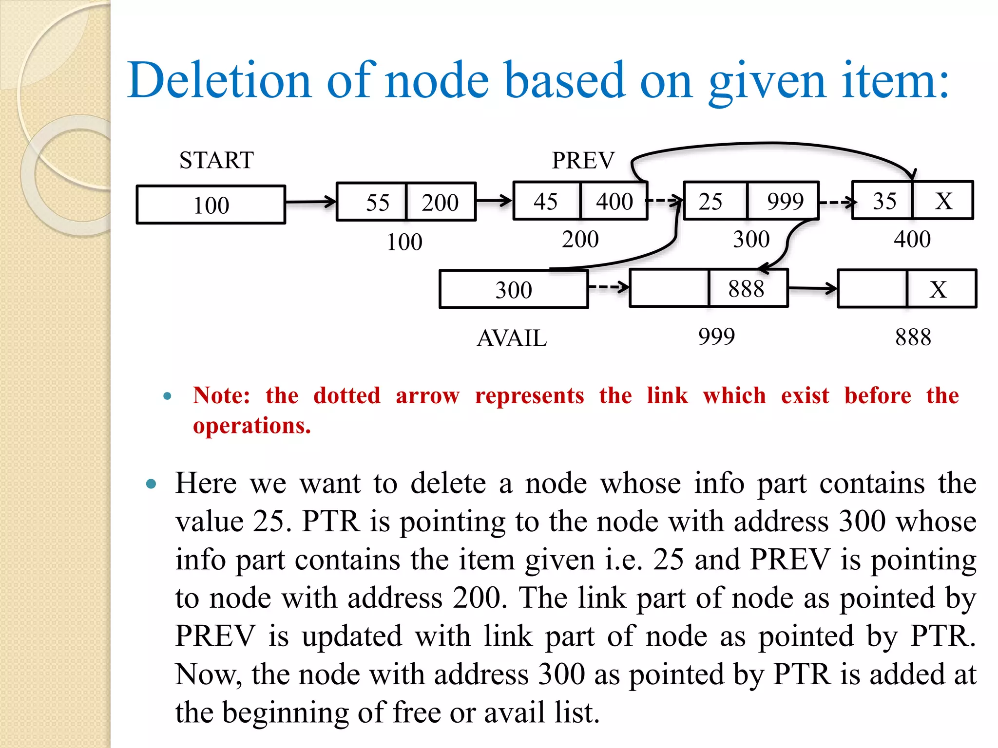
![Algorithm: Deletion_ITEM(START, LINK, INFO, PTR, PREV, AVAIL, ITEM) Step 1: PTR = START Step 2: Repeat while PTR != NULL AND ITEM != INFO[PTR] PREV = PTR PTR = LINK[PTR] [End of while] Step 3: if PTR = NULL, then display “Item not found”. Step 4: else if PTR = START, then START = LINK[PTR] Step 5: else LINK[PREV] = LINK[PTR] [End of if] Step 6: LINK[PTR] = AVAIL Step 7: AVAIL = PTR Step 8: exit](https://image.slidesharecdn.com/datastructureusingcmodule1-170525065731/75/Data-structure-using-c-module-1-135-2048.jpg)
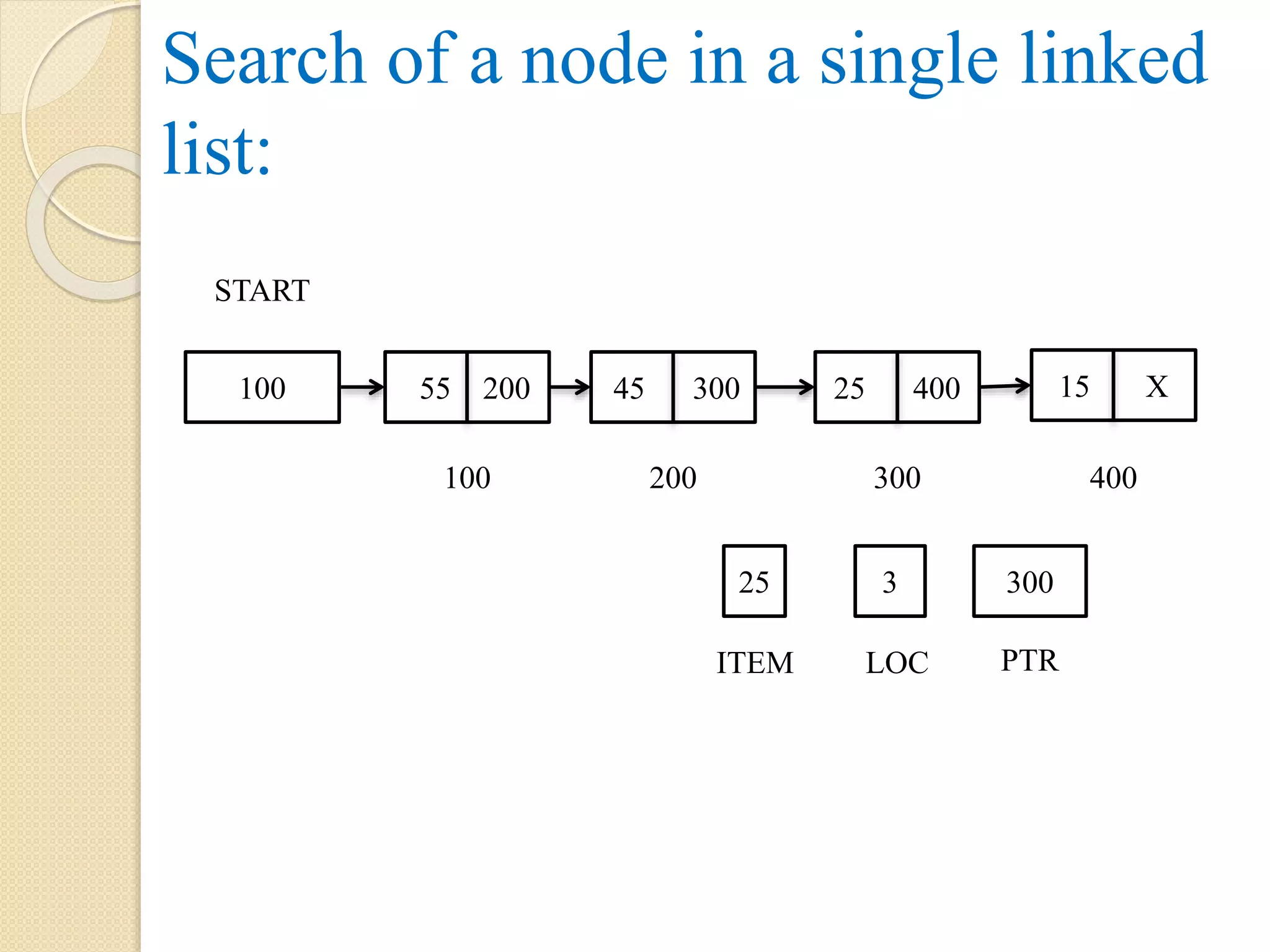
![Algorithm Search_Node(INFO, LINK, START, PTR, ITEM) Step 1: Let LOC = 0, F = 0 Step 2: PTR = START Step 3: Repeat while PTR != NULL ◦ Step 3.1: Set LOC = LOC + 1 ◦ Step 3.2: if ITEM = INFO[PTR], then F = 1 break [End of if] PTR = LINK[PTR] [End of while] Step 4: if F = 0, then display “Item not found”. Step 5: else display “Item found at Location”, LOC [End of if] Step 6: Exit](https://image.slidesharecdn.com/datastructureusingcmodule1-170525065731/75/Data-structure-using-c-module-1-137-2048.jpg)
![Concatenation of two single linked list: 50 200 100 20 300 30 111 200 300 100 START1 55 222 111 45 333 25 444 15 X 222 333 444 111 START2 PTR Step 1: Let PTR Step 2: PTR = START1 Step 3: Repeat while LINK[PTR] != NULL PTR = LINK[PTR] [End of while] Step 4: LINK[PTR] = START2 Step 5: START2 = NULL Step 6: Exit Algorithm:](https://image.slidesharecdn.com/datastructureusingcmodule1-170525065731/75/Data-structure-using-c-module-1-138-2048.jpg)
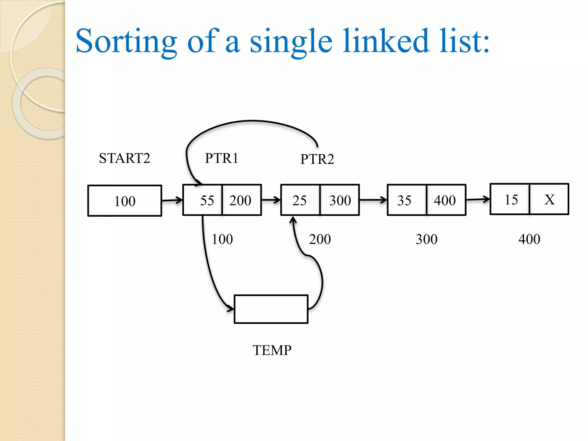
![Algorithm SORTING(START, INFO, LINK) Step 1: Let PTR1, PTR2, TEMP Step 2: PTR = START Step 3: Repeat while LINK[PTR] != NULL Step 3.1: PTR2 = LINK[PTR1] Step 3.2: Repeat while PTR2 != NULL Step 3.2.1: if INFO[PTR1] > INFO[PTR2], then TEMP = INFO[PTR1] INFO[PTR1] = INFO[PTR2] INFO[PTR2] = TEMP [End of if] PTR2 = LINK[PTR2] [End of while] PTR1 = LINK[PTR2] [End of while] Step 4: Exit](https://image.slidesharecdn.com/datastructureusingcmodule1-170525065731/75/Data-structure-using-c-module-1-140-2048.jpg)
![Reversing a Single Linked List: Reversing of single linked list means pointing the START pointer to the last node, then the last node link part have to point to its previous node and that node have to point to its previous node and so on till 1st node, where the 1st node link part will point to NULL. NULL 100 200 LINK[PTR] PREV PTR SAVE 100 55 200 100 START 45 300 25 400 15 X 200 300 400](https://image.slidesharecdn.com/datastructureusingcmodule1-170525065731/75/Data-structure-using-c-module-1-141-2048.jpg)
![ Here for each node identified by PTR is used to connect in reverse order. E.g. when PTR = 100, LINK[PTR] points to NULL as it becomes last node. Then PTR = SAVE to point to the next node. Finally we get the linked list as: 400 55 X 100 START 45 100 25 200 15 300 200 300 400 Info Link Info Link Info Link Info Link](https://image.slidesharecdn.com/datastructureusingcmodule1-170525065731/75/Data-structure-using-c-module-1-142-2048.jpg)
![Algorithm REVERSE(START, INFO, LINK) Step 1: Let PREV, SAVE, PTR Step 2: PTR = START Step 3: PREV = NULL Step 4: Repeat while PTR != NULL SAVE = LINK[PTR] LINK[PTR] = PREV PREV = PTR PTR = SAVE [End of while] Step 5: START = PREV Step 6: Exit](https://image.slidesharecdn.com/datastructureusingcmodule1-170525065731/75/Data-structure-using-c-module-1-143-2048.jpg)
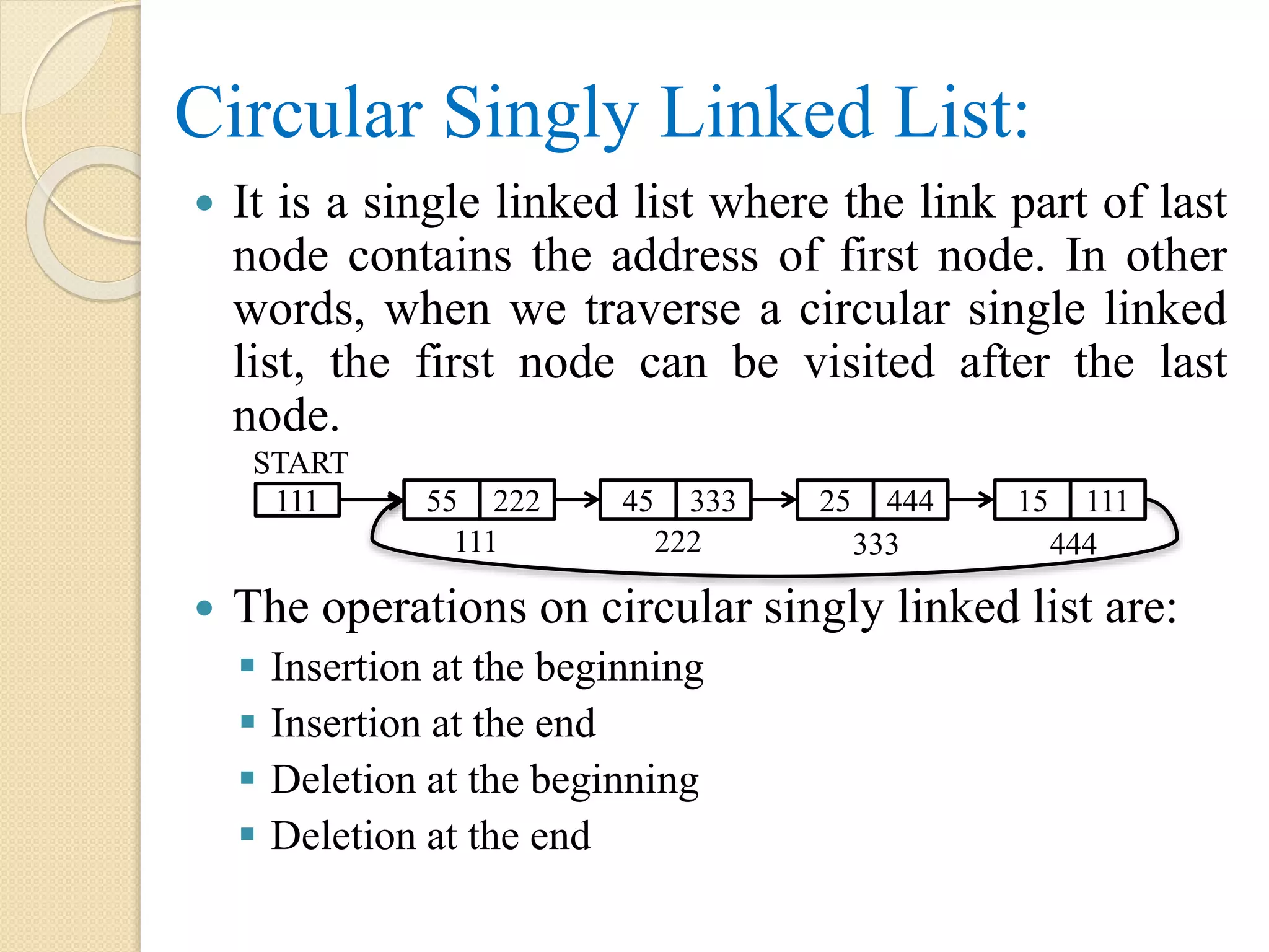
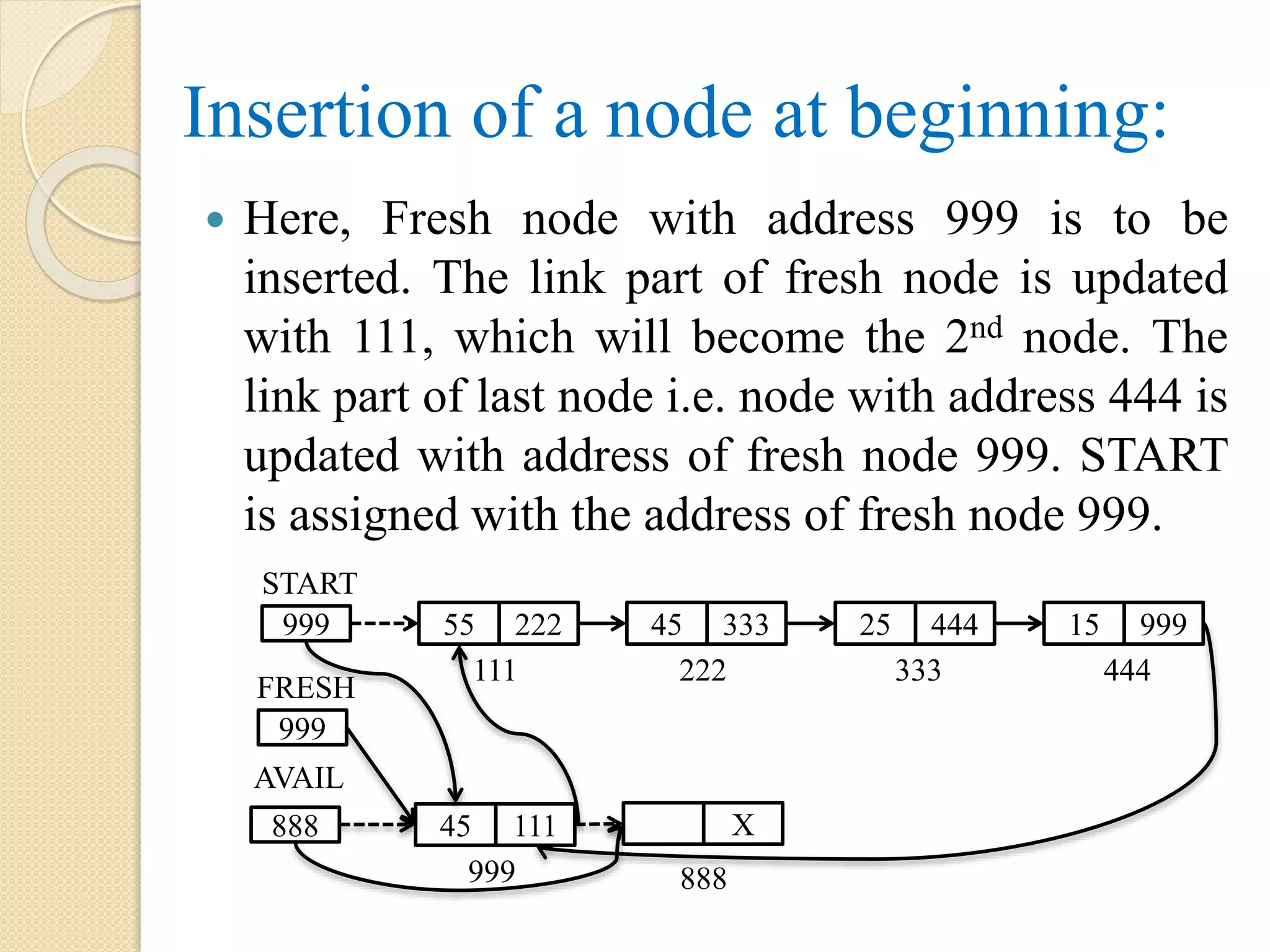
![Algorithm: INSERTFIRST(START, INFO, LINK, AVAIL, FRESH, ITEM) Step 1: if AVAIL = NULL, then Display “Memory Insufficient” Step 2: else FRESH = AVAIL AVAIL = LINK[AVAIL] INFO[FRESH] = ITEM LINK[FRESH] = NULL Step 2.1: if START = NULL, then START = FRESH LINK[FRESH] = START](https://image.slidesharecdn.com/datastructureusingcmodule1-170525065731/75/Data-structure-using-c-module-1-146-2048.jpg)
![◦ Step 2.2: else LINK[FRESH] = START PTR = START Repeat while(LINK[PTR] != START) PTR = LINK[PTR] [End of while] LINK[PTR] = FRESH START = FRESH [End of if] Step 3: Exit](https://image.slidesharecdn.com/datastructureusingcmodule1-170525065731/75/Data-structure-using-c-module-1-147-2048.jpg)
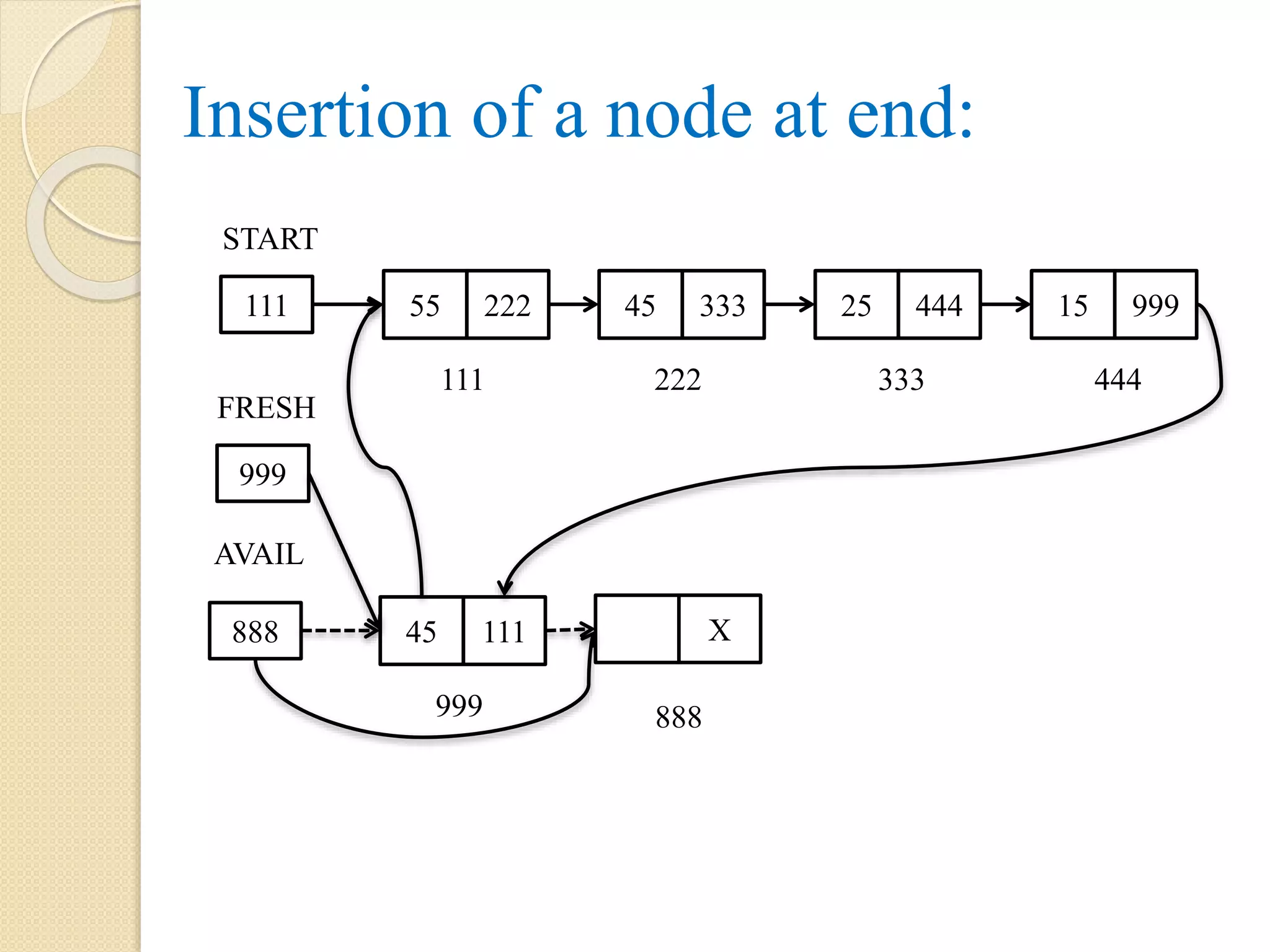
![Algorithm: INSERTEND(START, INFO, LINK, AVAIL, FRESH, ITEM) Step 1: if AVAIL = NULL, then Display “Memory Insufficient” Step 2: else FRESH = NULL AVAIL = LINK[AVAIL] INFO[FRESH] = ITEM LINK[FRESH] = NULL Step 2.1: if START = NULL, then START = FRESH LINK[FRESH] = START](https://image.slidesharecdn.com/datastructureusingcmodule1-170525065731/75/Data-structure-using-c-module-1-149-2048.jpg)
![◦ Step 2.2: else PTR = START Repeat while(LINK[PTR] != START) PTR = LINK[PTR] [End of while] LINK[PTR] = FRESH LINK[FRESH] = START [End of if Step 2.1] [End of if – Step 1 ] Step 3: Exit](https://image.slidesharecdn.com/datastructureusingcmodule1-170525065731/75/Data-structure-using-c-module-1-150-2048.jpg)
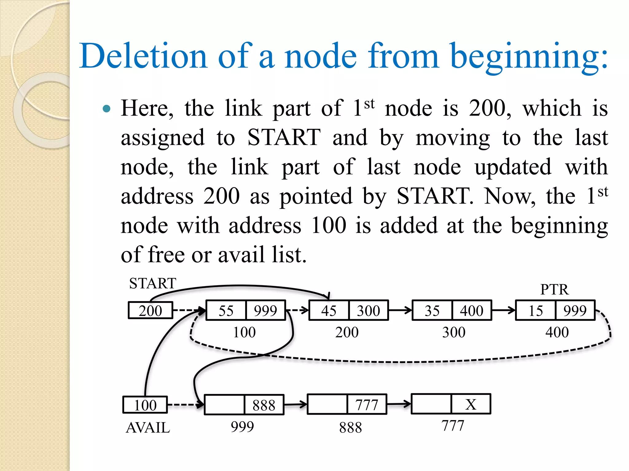
![Algorithm: DELETEFIRST(START, INFO, LINK, AVAIL) Step 1: if START = NULL, then Display “List does not exist” Step 2: else if START = LINK[START], then LINK[START] = AVAIL AVAIL = START START = NULL Step 3: else PTR = START](https://image.slidesharecdn.com/datastructureusingcmodule1-170525065731/75/Data-structure-using-c-module-1-152-2048.jpg)
![Repeat while (LINK[PTR] != START) PTR = LINK[PTR] [End of while] LINK[PTR] = LINK[START] PTR = START START = LINK[START] LINK[PTR] = AVAIL AVAIL = PTR [End of if] Step 4: Exit](https://image.slidesharecdn.com/datastructureusingcmodule1-170525065731/75/Data-structure-using-c-module-1-153-2048.jpg)
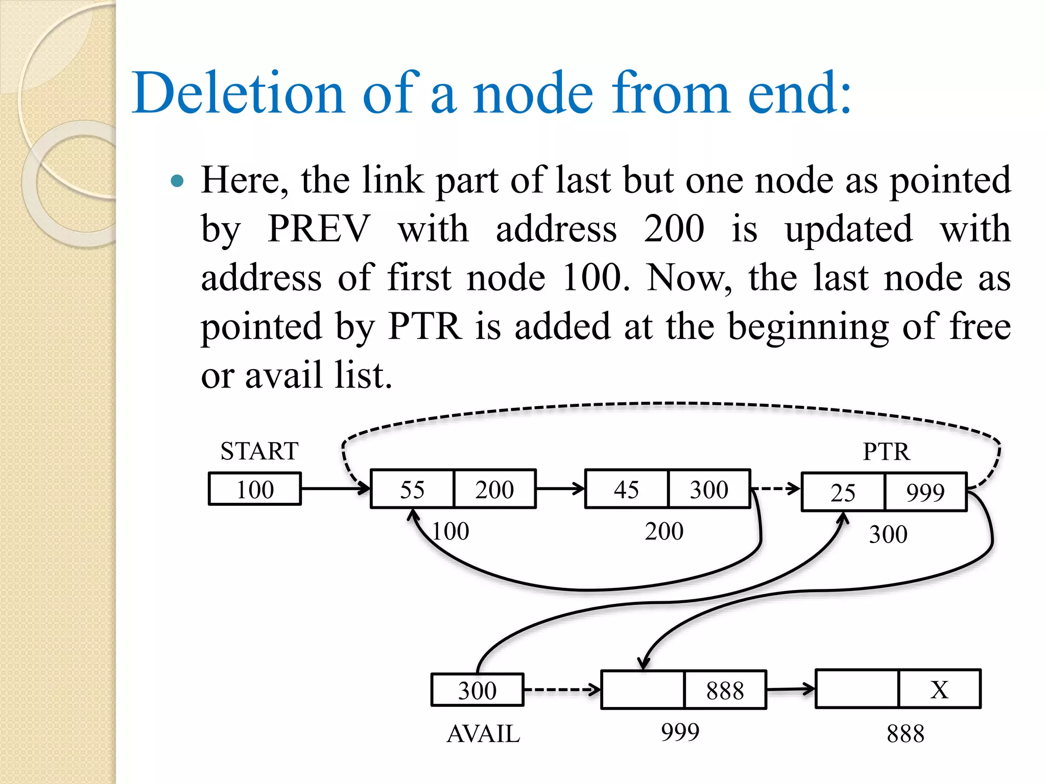
![Algorithm: DELETEEND(START, INFO, LINK, AVAIL) Step 1: if START = NULL, then Display “List does not exist” Step 2: else if START = LINK[START], then LINK[START] = AVAIL AVAIL = START START = NULL Step 3: else PTR = START](https://image.slidesharecdn.com/datastructureusingcmodule1-170525065731/75/Data-structure-using-c-module-1-155-2048.jpg)
![Repeat while (LINK[PTR] != START) PREV = PTR PTR = LINK[PTR] [End of while] LINK[PREV] = START LINK[PTR] = AVAIL AVAIL = PTR [End of if] Step 4: Exit](https://image.slidesharecdn.com/datastructureusingcmodule1-170525065731/75/Data-structure-using-c-module-1-156-2048.jpg)
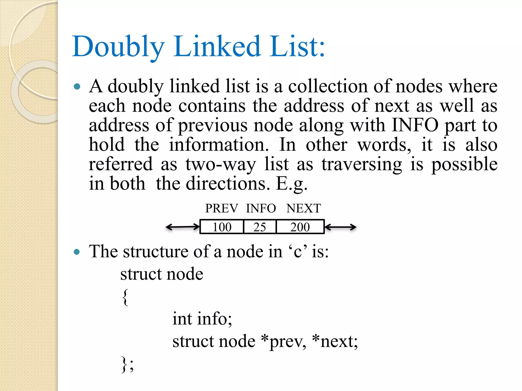
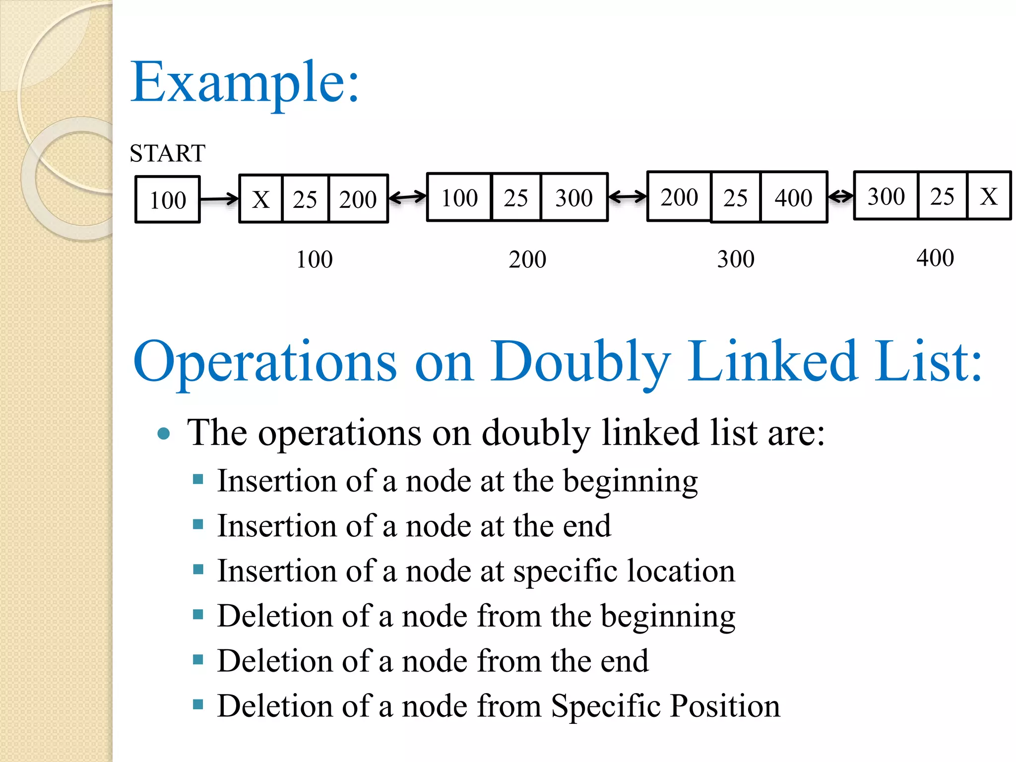
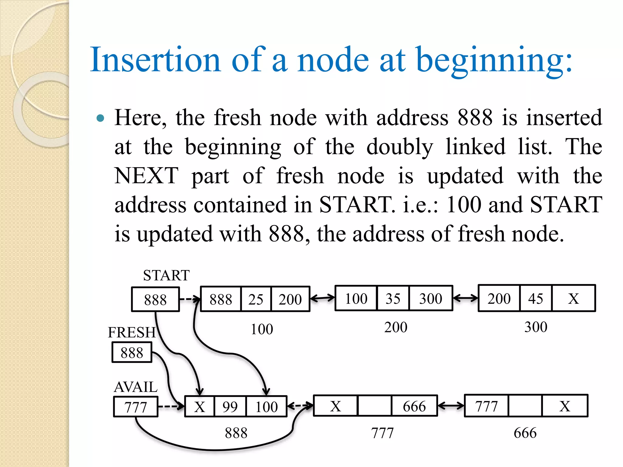
![Algorithm: INSERTFIRST(START, INFO, NEXT, PREV, AVAIL, FRESH) Step 1: if AVAIL = NULL, then Display “Memory Insufficient” Step 2: else FRESH = AVAIL AVAIL = NEXT[AVAIL] PREV[AVAIL] = NULL NEXT[FRESH] = NULL PREV[FRESH] = NULL INFO[FRESH] = ITEM](https://image.slidesharecdn.com/datastructureusingcmodule1-170525065731/75/Data-structure-using-c-module-1-161-2048.jpg)
![ Step 2.1: if START = NULL, then START = FRESH Step 2.2: else NEXT[FRESH] = START PREV[START] = FRESH START = FRESH [End of if – Step 2.1] [End of if – Step – 1] Step 3: Exit](https://image.slidesharecdn.com/datastructureusingcmodule1-170525065731/75/Data-structure-using-c-module-1-162-2048.jpg)
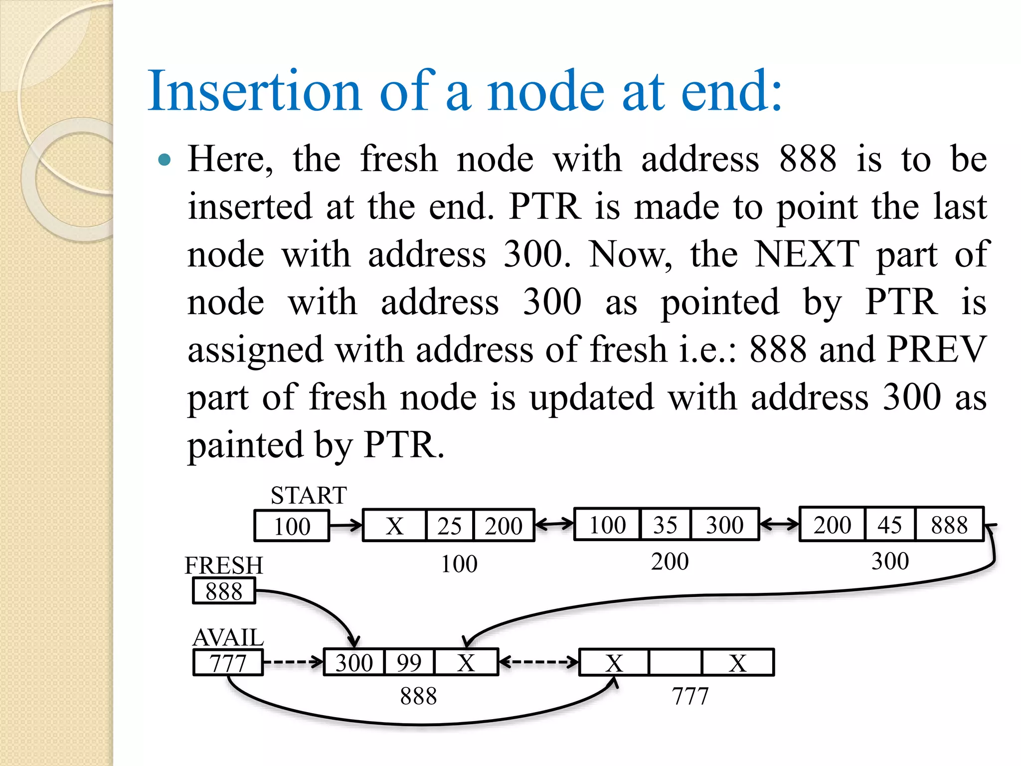
![Algorithm: INSERTEND(START, INFO, NEXT, PREV, AVAIL, FRESH, PTR) Step 1: if AVAIL = NULL, then Display “Memory Insufficient” Step 2: else FRESH = AVAIL AVAIL = NEXT[AVAIL] PREV[AVAIL] = NULL NEXT[FRESH] = NULL PREV[FRESH] = NULL INFO[FRESH] = ITEM](https://image.slidesharecdn.com/datastructureusingcmodule1-170525065731/75/Data-structure-using-c-module-1-164-2048.jpg)
![ Step 2.1: if START = NULL, then START = FRESH Step 2.2: else PTR = START while NEXT[PTR] != NULL PTR = NEXT[PTR] [End of while] NEXT[PTR] = FRESH PREV[FRESH] = PTR START = FRESH [End of if – Step 2.1] [End of if – Step – 1] Step 3: Exit](https://image.slidesharecdn.com/datastructureusingcmodule1-170525065731/75/Data-structure-using-c-module-1-165-2048.jpg)
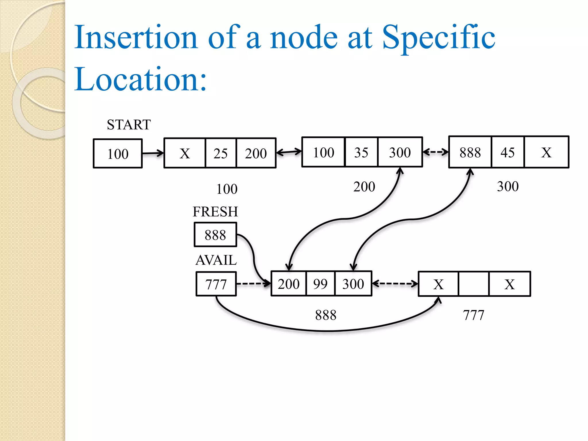
![Algorithm: INSERTATLOC(START, INFO, NEXT, PREV, AVAIL, FRESH, PTR) Step 1: if AVAIL = NULL, then Display “Memory Insufficient” Step 2: else FRESH = AVAIL AVAIL = NEXT[AVAIL] PREV[AVAIL] = NULL NEXT[FRESH] = NULL PREV[FRESH] = NULL INFO[FRESH] = ITEM](https://image.slidesharecdn.com/datastructureusingcmodule1-170525065731/75/Data-structure-using-c-module-1-167-2048.jpg)
![ Step 2.1: if START = NULL, then START = FRESH Step 2.2: else Step 2.2.1: Set I = 1, PTR1 = START Step 2.2.2: Repeat while I < LOC AND PTR1 = NULL Set PTR = PTR1 Set PTR1 = NEXT[PTR1] Set I = I + 1 [End of while] Step 2.2.3: if PTR1 = NULL, then Display “ Location does not exist”. Step 2.2.4: else if PTR 1 = START, then NEXT[FRESH] = START PREV[START] = FRESH](https://image.slidesharecdn.com/datastructureusingcmodule1-170525065731/75/Data-structure-using-c-module-1-168-2048.jpg)
![ Step 2.2.5: else NEXT[PTR] = FRESH PREV[FRESH] = PTR NEXT[FRESH] = PTR1 PREV[PTR1] = FRESH [End of if – Step 2.2.3] [End of if – Step – 2.1] [End of if – Step – 1] Step 3: Exit](https://image.slidesharecdn.com/datastructureusingcmodule1-170525065731/75/Data-structure-using-c-module-1-169-2048.jpg)
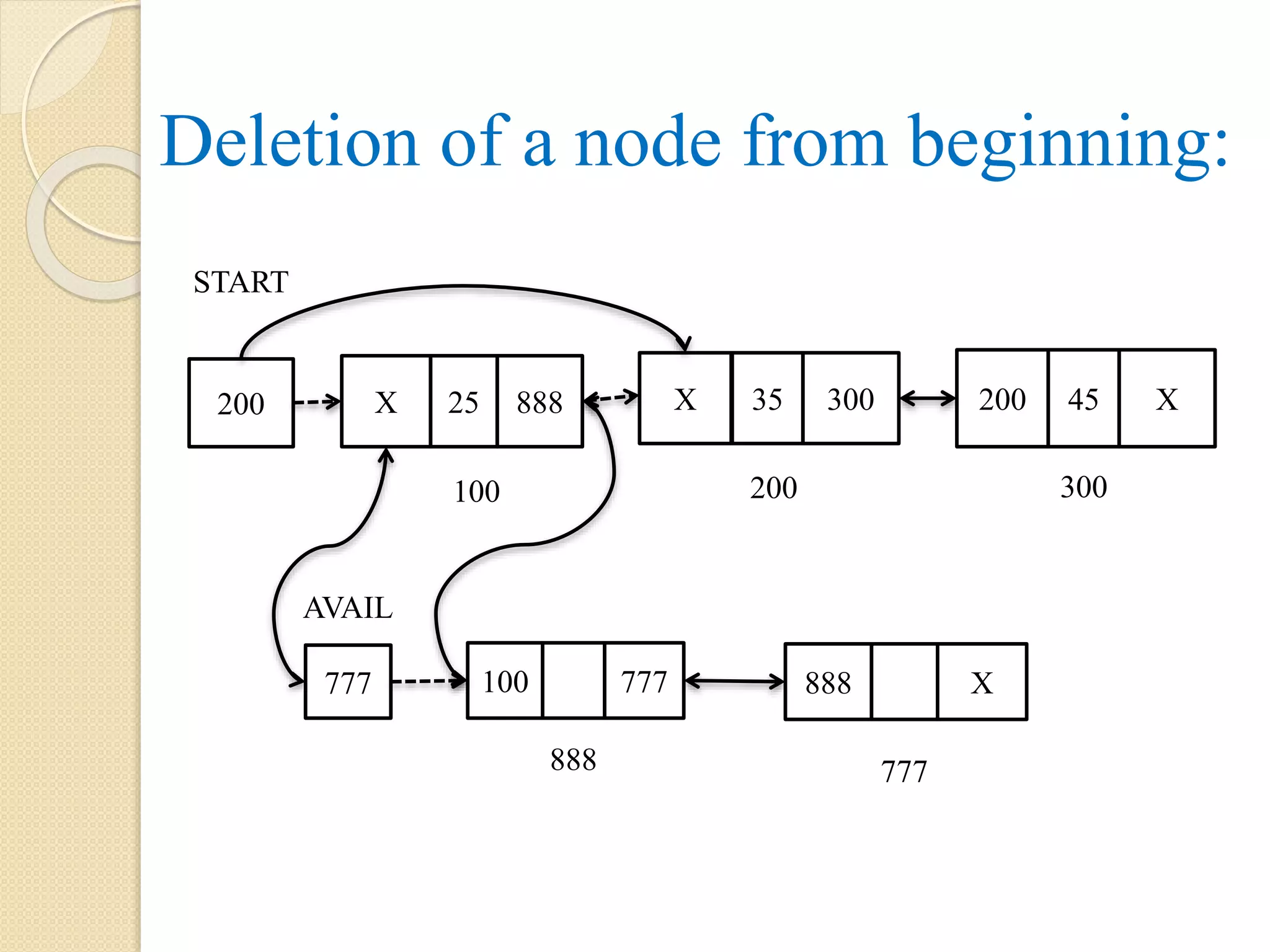
![Algorithm: DELETEFIRST(START, NEXT, PREV, AVAIL, PTR) Step 1: if START = NULL, then Display “List does not exist” Step 2: else PTR = START START = NEXT[PTR] NEXT[PTR] = AVAIL PREV[AVAIL] = PTR AVAIL = PTR [End of if] Step 3: Exit](https://image.slidesharecdn.com/datastructureusingcmodule1-170525065731/75/Data-structure-using-c-module-1-171-2048.jpg)
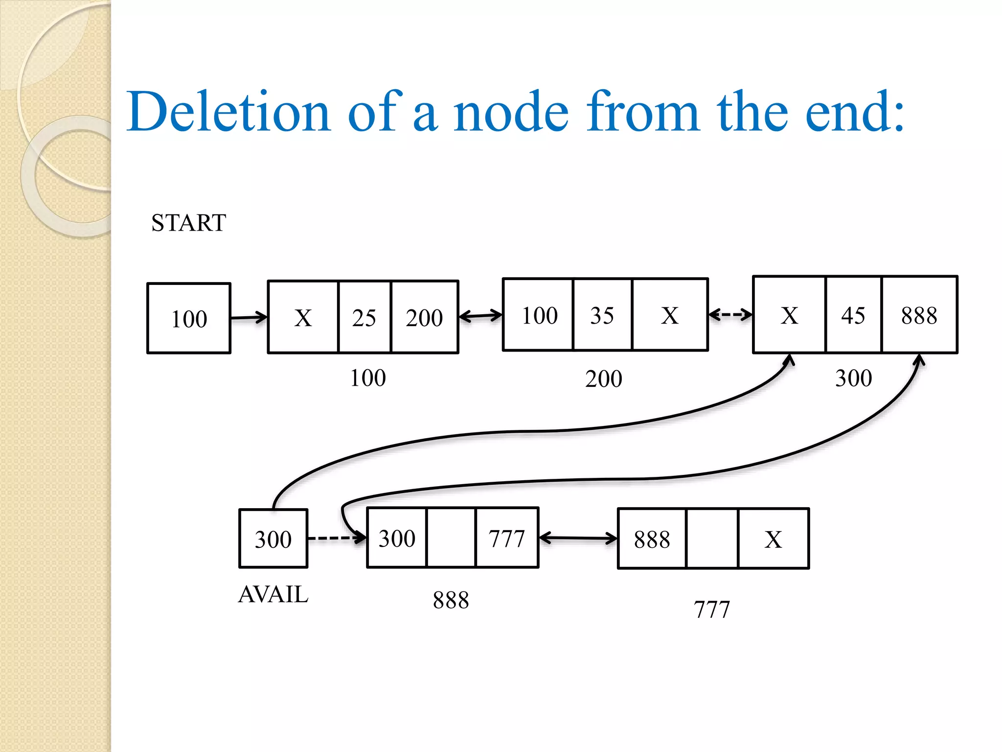
![Algorithm: DELETEEND(START, NEXT, PREV, AVAIL, PTR) Step 1: if START = NULL, then Display “List does not exist” Step 2: else Step 2.1: PTR1 = START Step 2.2: Repeat while NEXT[PTR] != NULL Set PTR = PTR1 Set PTR1 = NEXT[PTR1] [End of while]](https://image.slidesharecdn.com/datastructureusingcmodule1-170525065731/75/Data-structure-using-c-module-1-173-2048.jpg)
![ Step 2.3: NEXT[PTR] = NULL PREV[PTR1] = NULL NEXT[PTR1] = AVAIL PREV[AVAIL] = PTR1 AVAIL = PTR1 [End of if] Step 3: Exit](https://image.slidesharecdn.com/datastructureusingcmodule1-170525065731/75/Data-structure-using-c-module-1-174-2048.jpg)
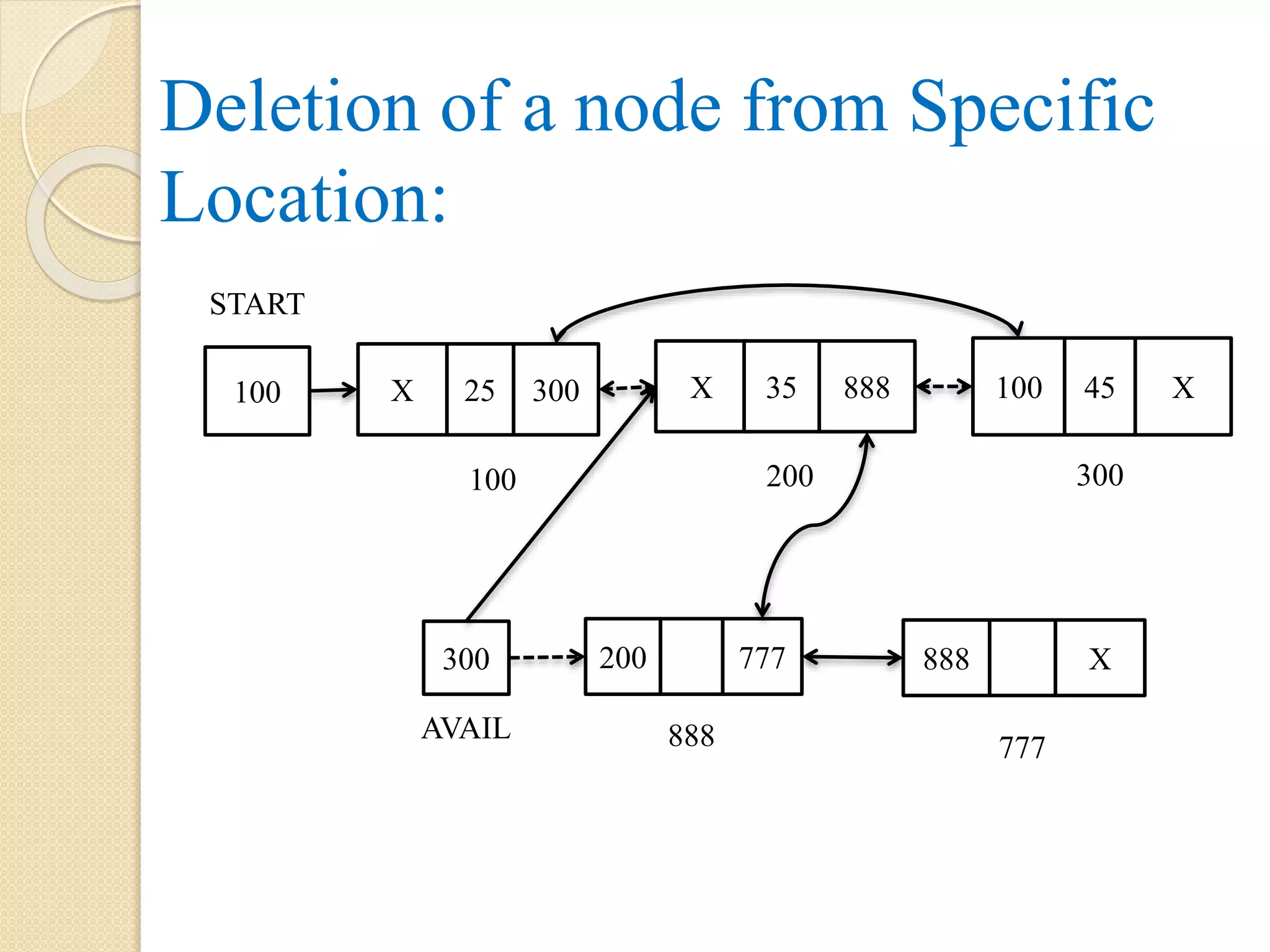
![Algorithm: DELETEPOS(START, LOC, PTR, PTR1, ITEM, AVAIL) Step 1: Let I = 1 Step 2: if START = NULL, then Display “List does not exist” Step 3: else Step 3.1: PTR1 = START Step 3.2: Repeat while I < LOC AND PTR1 != NULL PTR = PTR1 PTR1 = NEXT[PTR1]](https://image.slidesharecdn.com/datastructureusingcmodule1-170525065731/75/Data-structure-using-c-module-1-176-2048.jpg)
![I = I + 1 [End of while] Step 3.3: if PTR1 = NULL, then Display “Location entered not exist” Step 3.4: else if PTR1 = START, then START = NEXT[START] PREV[START] = NULL Step 3.5: else if NEXT[PTR1] = NULL, then NEXT[PTR] = NULL](https://image.slidesharecdn.com/datastructureusingcmodule1-170525065731/75/Data-structure-using-c-module-1-177-2048.jpg)
![ Step 3.6: else NEXT[PTR] = NEXT[PTR1] PREV[NEXT[PTR1]] = PTR [End of Step 3.3] Step 3.7: NEXT[PTR1] = AVAIL PREV[AVAIL] = PTR1 PREV[PTR1] = NULL AVAIL = PTR1 [End of Step – 2] Step 3: Exit](https://image.slidesharecdn.com/datastructureusingcmodule1-170525065731/75/Data-structure-using-c-module-1-178-2048.jpg)
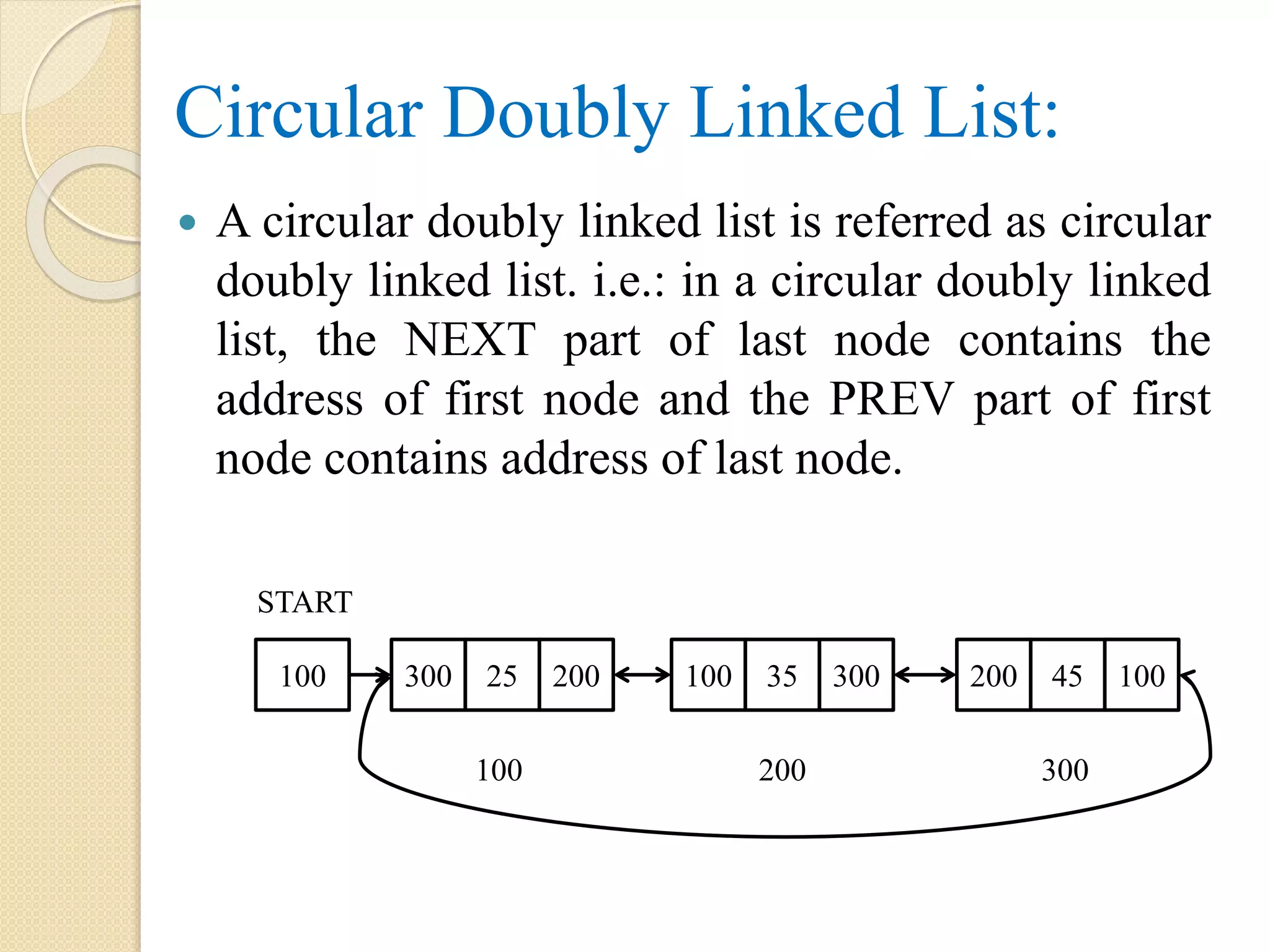
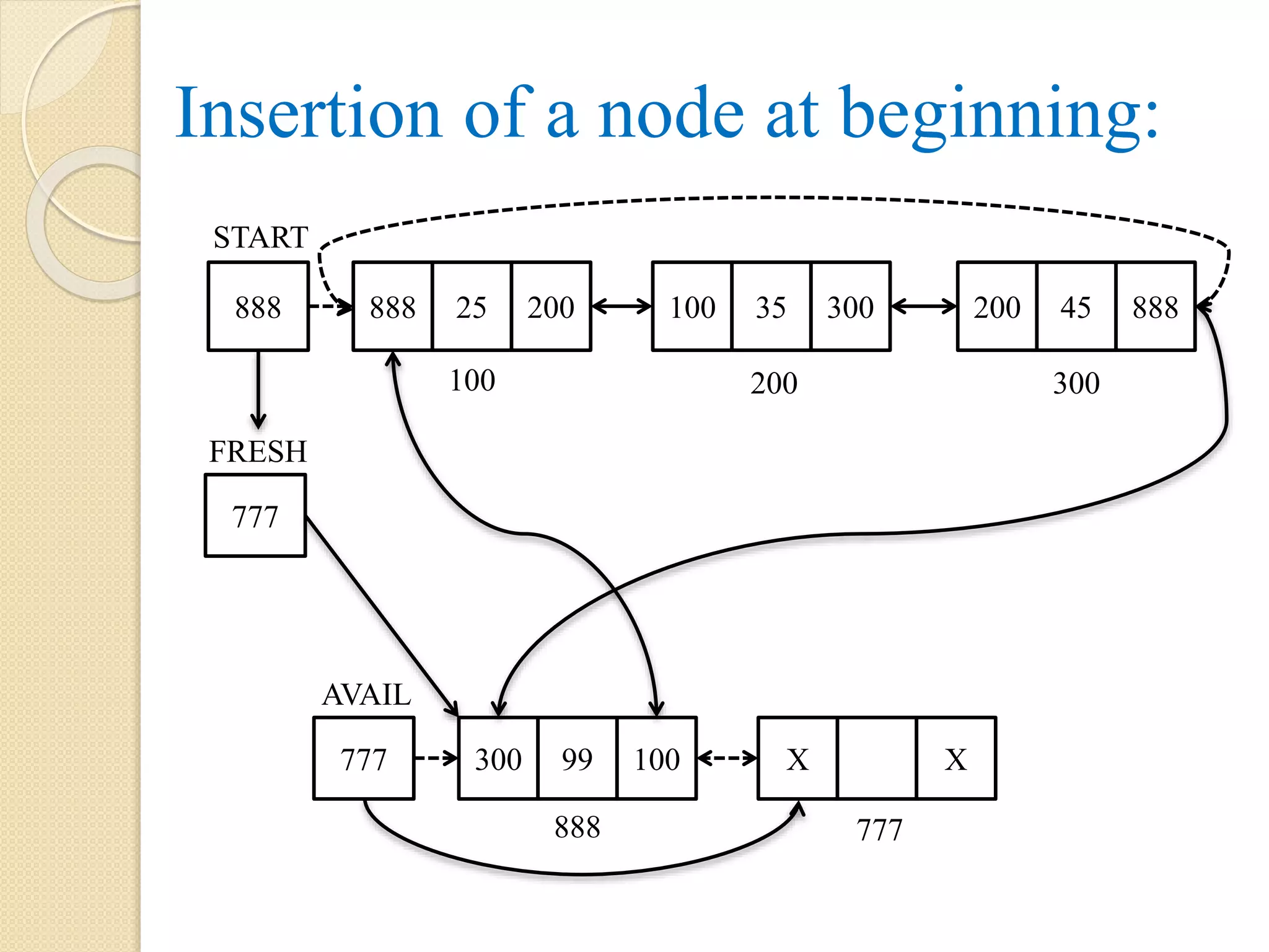
![Algorithm: INSERTFIRST(START, FRESH, INFO, PREV, NEXT, PTR, AVAIL) Step 1: if AVAIL = NULL, then Display “insufficient memory” Step 2: else Step 2.1: FRESH = AVAIL AVAIL = NEXT[AVAIL] PREV[AVAIL] = NULL PREV[FRESH] = NULL NEXT[FRESH] = NULL](https://image.slidesharecdn.com/datastructureusingcmodule1-170525065731/75/Data-structure-using-c-module-1-181-2048.jpg)
![ Step 2.2: if START = NULL, then START = FRESH PREV[FRESH] = START NEXT[FRESH] = START Step 2.3: else PTR = PREV[START] NEXT[PTR] = FRESH PREV[FRESH] = PTR NEXT[FRESH] = START PREV[START] = FRESH START = FRESH [End of if] [End of if] Step 3: Exit](https://image.slidesharecdn.com/datastructureusingcmodule1-170525065731/75/Data-structure-using-c-module-1-182-2048.jpg)
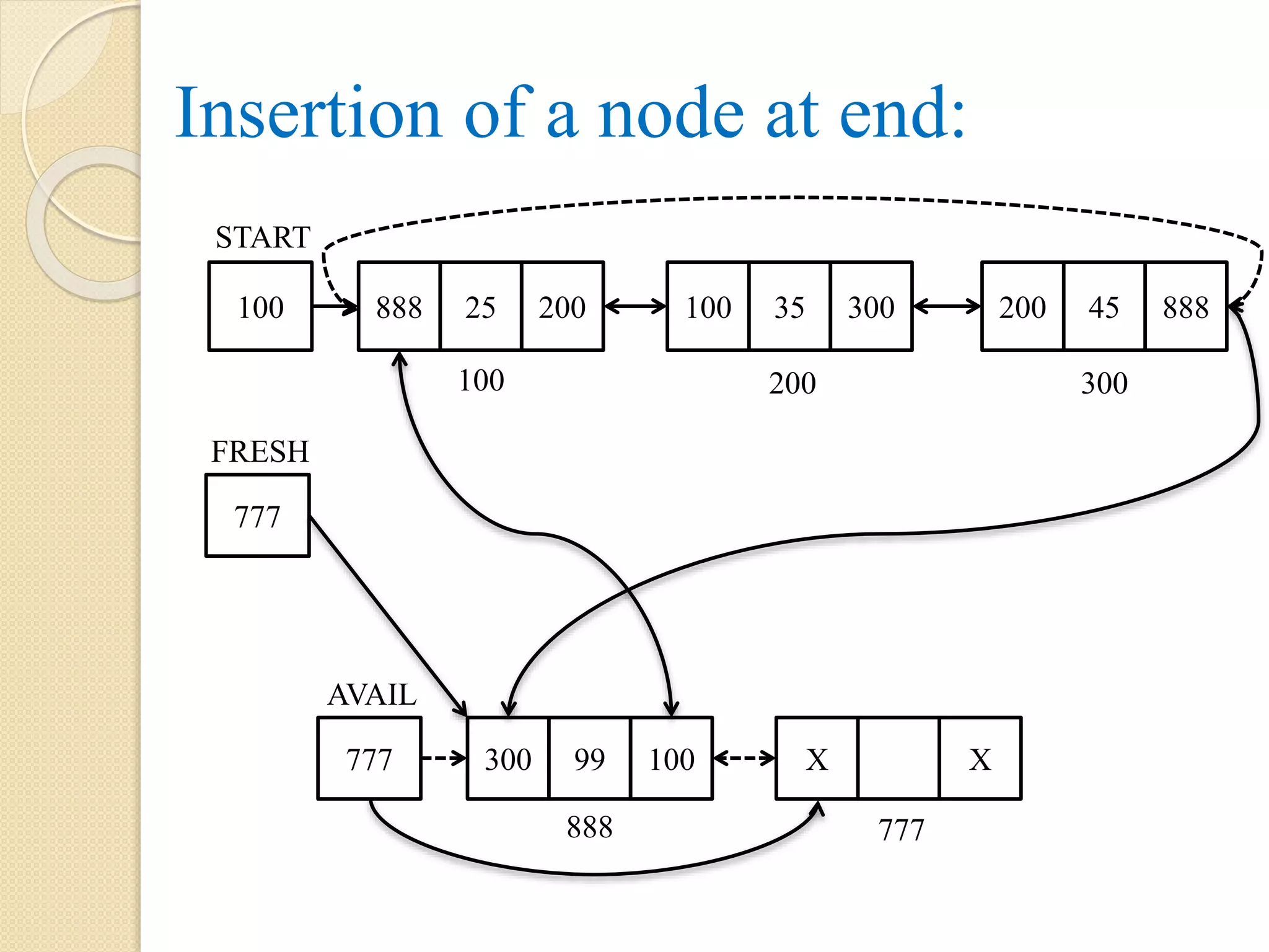
![Algorithm: INSERTEND(START, FRESH, INFO, PREV, NEXT, PTR, AVAIL) Step 1: if AVAIL = NULL, then Display “insufficient memory” Step 2: else Step 2.1: FRESH = AVAIL AVAIL = NEXT[AVAIL] PREV[AVAIL] = NULL PREV[FRESH] = NULL NEXT[FRESH] = NULL](https://image.slidesharecdn.com/datastructureusingcmodule1-170525065731/75/Data-structure-using-c-module-1-184-2048.jpg)
![ Step 2.2: if START = NULL, then START = FRESH PREV[FRESH] = START NEXT[FRESH] = START Step 2.3: else PTR = PREV[START] NEXT[PTR] = FRESH PREV[FRESH] = PTR NEXT[FRESH] = START PREV[START] = FRESH [End of if] [End of if] Step 3: Exit](https://image.slidesharecdn.com/datastructureusingcmodule1-170525065731/75/Data-structure-using-c-module-1-185-2048.jpg)
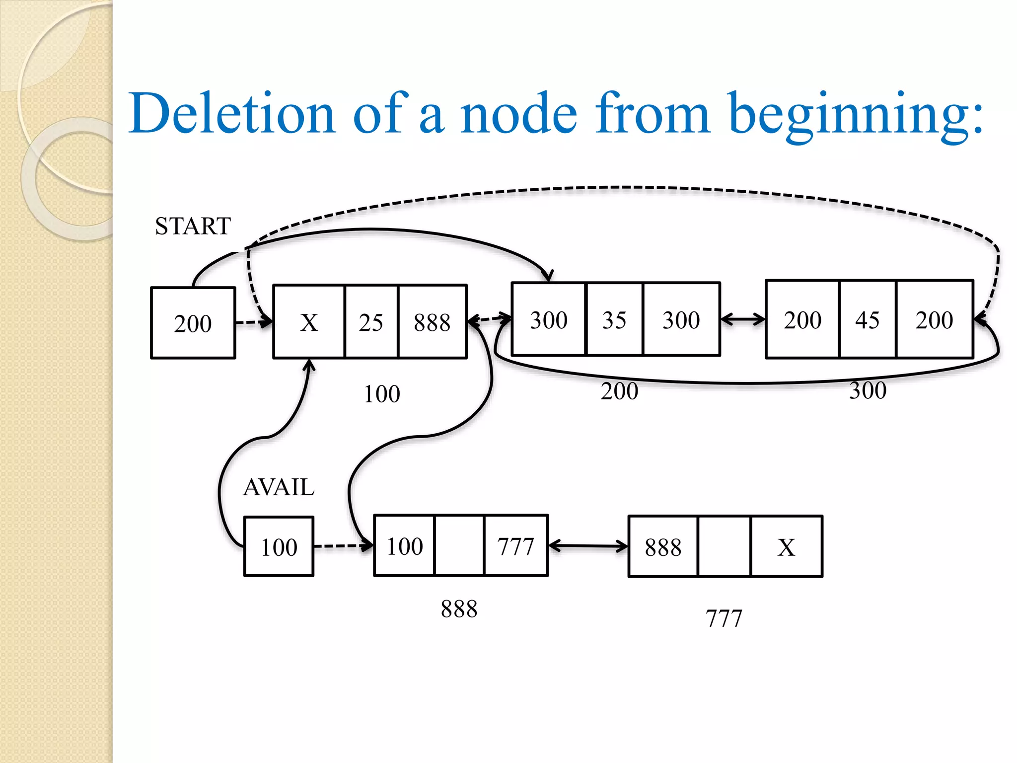
![Algorithm: DELETEFIRST(START, PTR, PTR1, PREV, NEXT, AVAIL) Step 1: if START = NULL, then Display “List does not exist” Step 2: else if NEXT[START] = START, then PTR = START START = NULL NEXT[PTR] = AVAIL PREV[AVAIL] = PTR AVAIL = PTR [End of if] Step 3: Exit](https://image.slidesharecdn.com/datastructureusingcmodule1-170525065731/75/Data-structure-using-c-module-1-187-2048.jpg)
![ Step 3: else PTR = PREV[START] PTR1 = START NEXT[PTR] = NEXT[PTR1] START = NEXT[PTR1] PREV[START] = PTR NEXT[PTR1] = AVAIL PREV[AVAIL] = PTR1 AVAIL = PTR1 [End of if] Step 4: Exit](https://image.slidesharecdn.com/datastructureusingcmodule1-170525065731/75/Data-structure-using-c-module-1-188-2048.jpg)
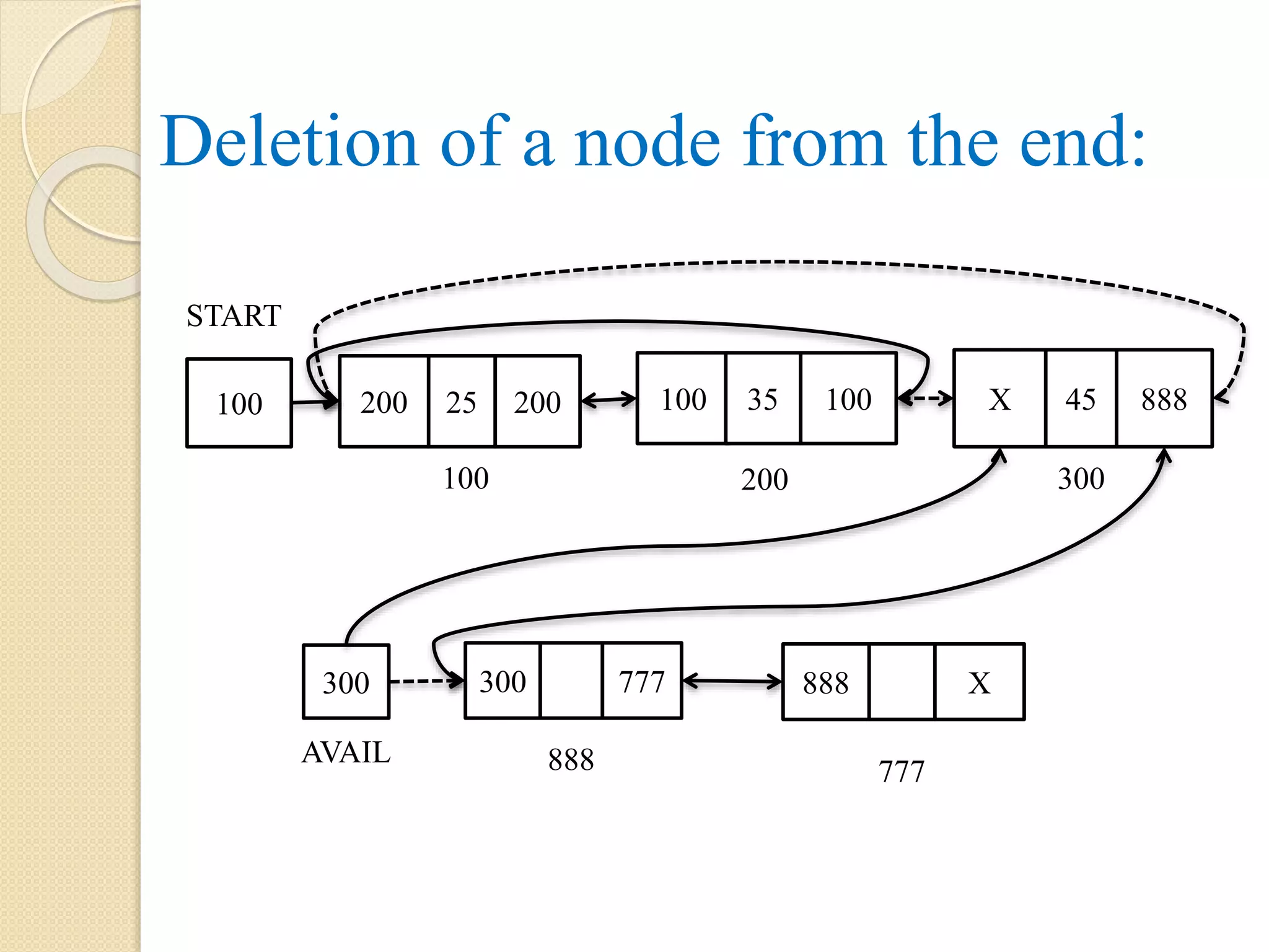
![Algorithm: DELETEEND(START, PTR, PTR1, PREV, NEXT, AVAIL) Step 1: if START = NULL, then Display “List does not exist” Step 2: else if START = NEXT[START], then PTR = START START = NULL NEXT[PTR] = AVAIL PREV[AVAIL] = PTR AVAIL = PTR](https://image.slidesharecdn.com/datastructureusingcmodule1-170525065731/75/Data-structure-using-c-module-1-190-2048.jpg)
![ Step 3: else PTR1 = PREV[START] PTR = PREV[PTR1] NEXT[PTR] = START PREV[START] = PTR NEXT[PTR1] = AVAIL PREV[AVAIL] = PTR1 AVAIL = PTR1 [End of if] Step 4: Exit](https://image.slidesharecdn.com/datastructureusingcmodule1-170525065731/75/Data-structure-using-c-module-1-191-2048.jpg)
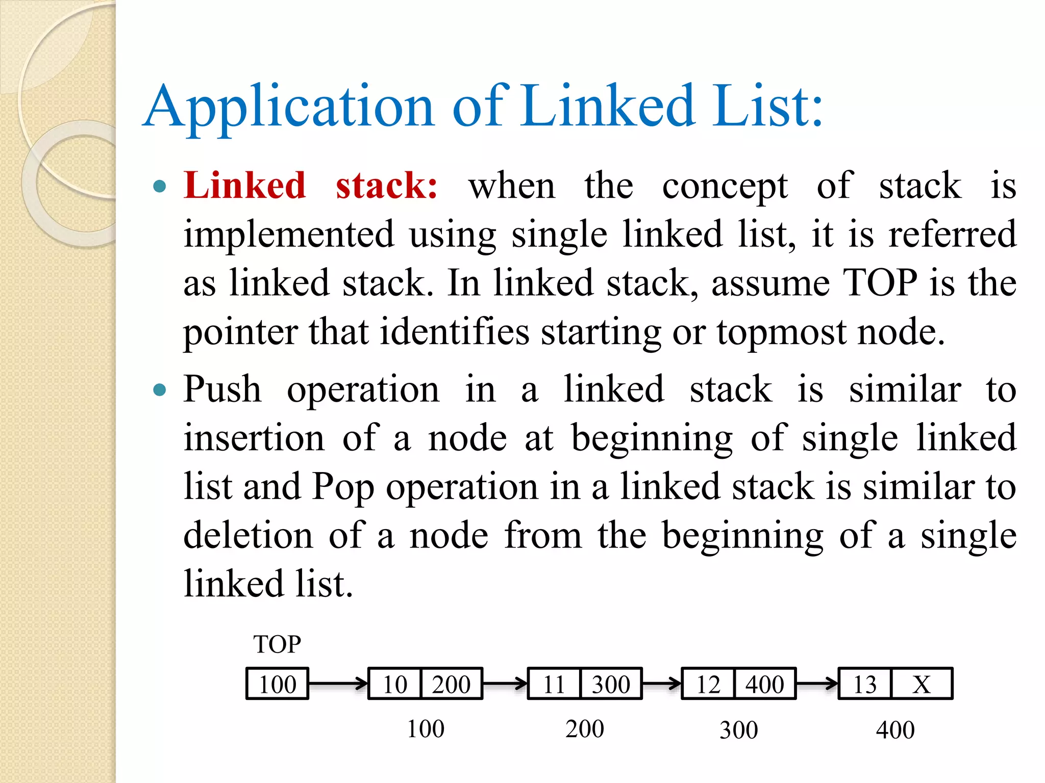
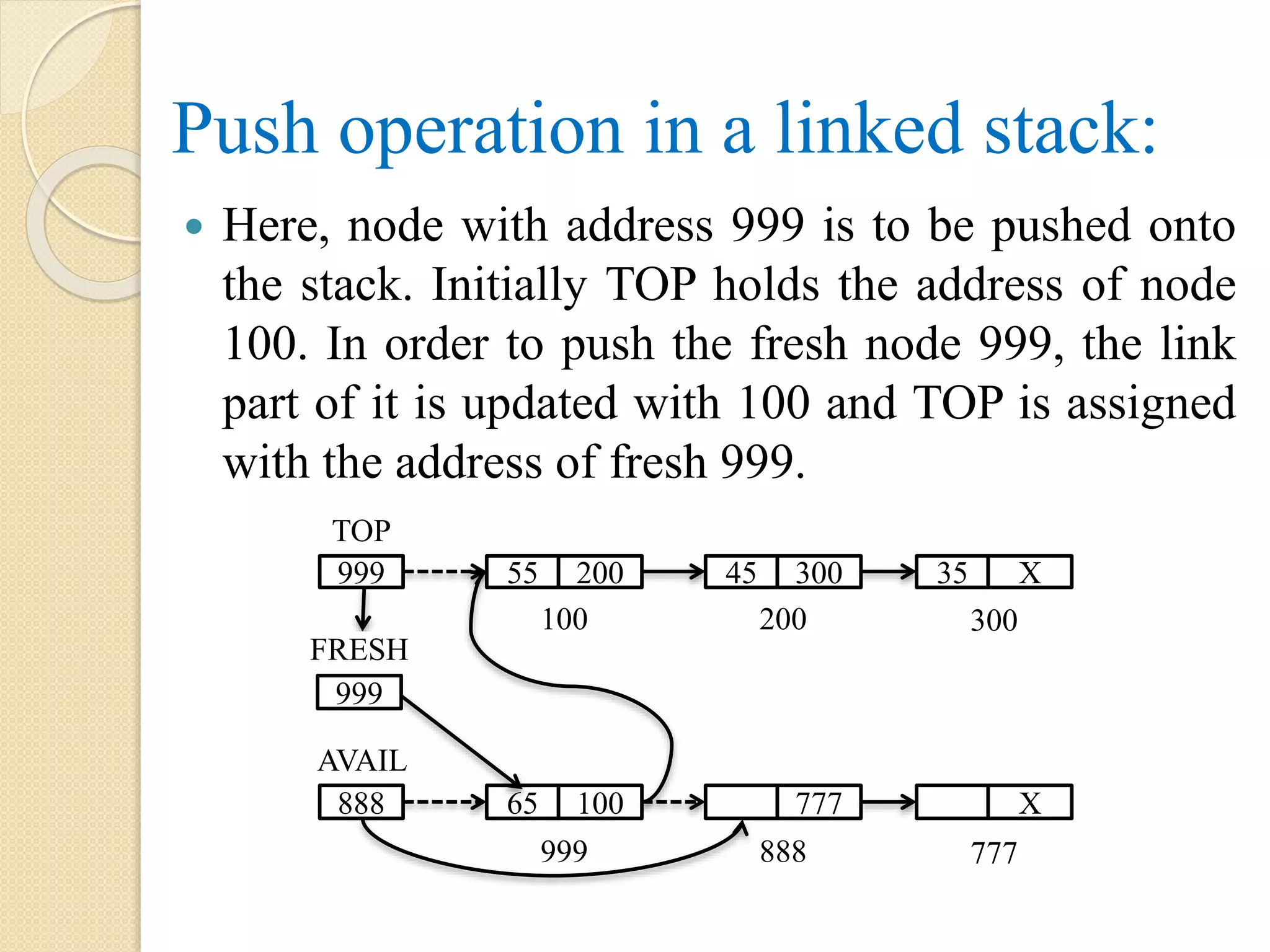
![Algorithm: PUSH(AVAIL, FRESH, LINK, INFO, TOP) Step 1: if AVAIL = NULL, then Display “Insufficient Memory” Step 2: else FRESH = AVAIL AVAIL = LINK[AVAIL] LINK[FRESH] = NULL INFO[FRESH] = ITEM Step 2.1: if TOP = NULL, then TOP = FRESH](https://image.slidesharecdn.com/datastructureusingcmodule1-170525065731/75/Data-structure-using-c-module-1-194-2048.jpg)
![ Step 2.2: else LINK[FRESH] = TOP TOP = FRESH [End of if – Step 2.1] [End of if – Step 1] Step 3: Exit](https://image.slidesharecdn.com/datastructureusingcmodule1-170525065731/75/Data-structure-using-c-module-1-195-2048.jpg)
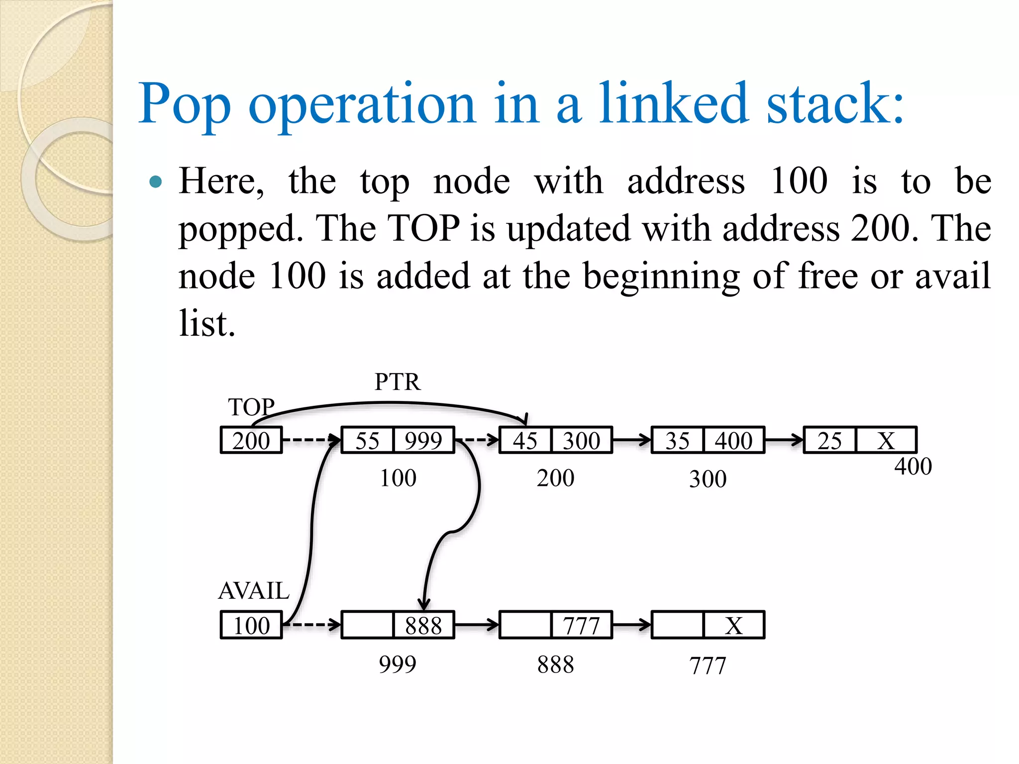
![Algorithm: PUSH(TOP, PTR, LINK, AVAIL) Step 1: if TOP = NULL, then Display “Underflow” Step 2: else PTR = TOP TOP = LINK[TOP] LINK[PTR] = AVAIL AVAIL = PTR [End of if] Step 3: Exit](https://image.slidesharecdn.com/datastructureusingcmodule1-170525065731/75/Data-structure-using-c-module-1-197-2048.jpg)
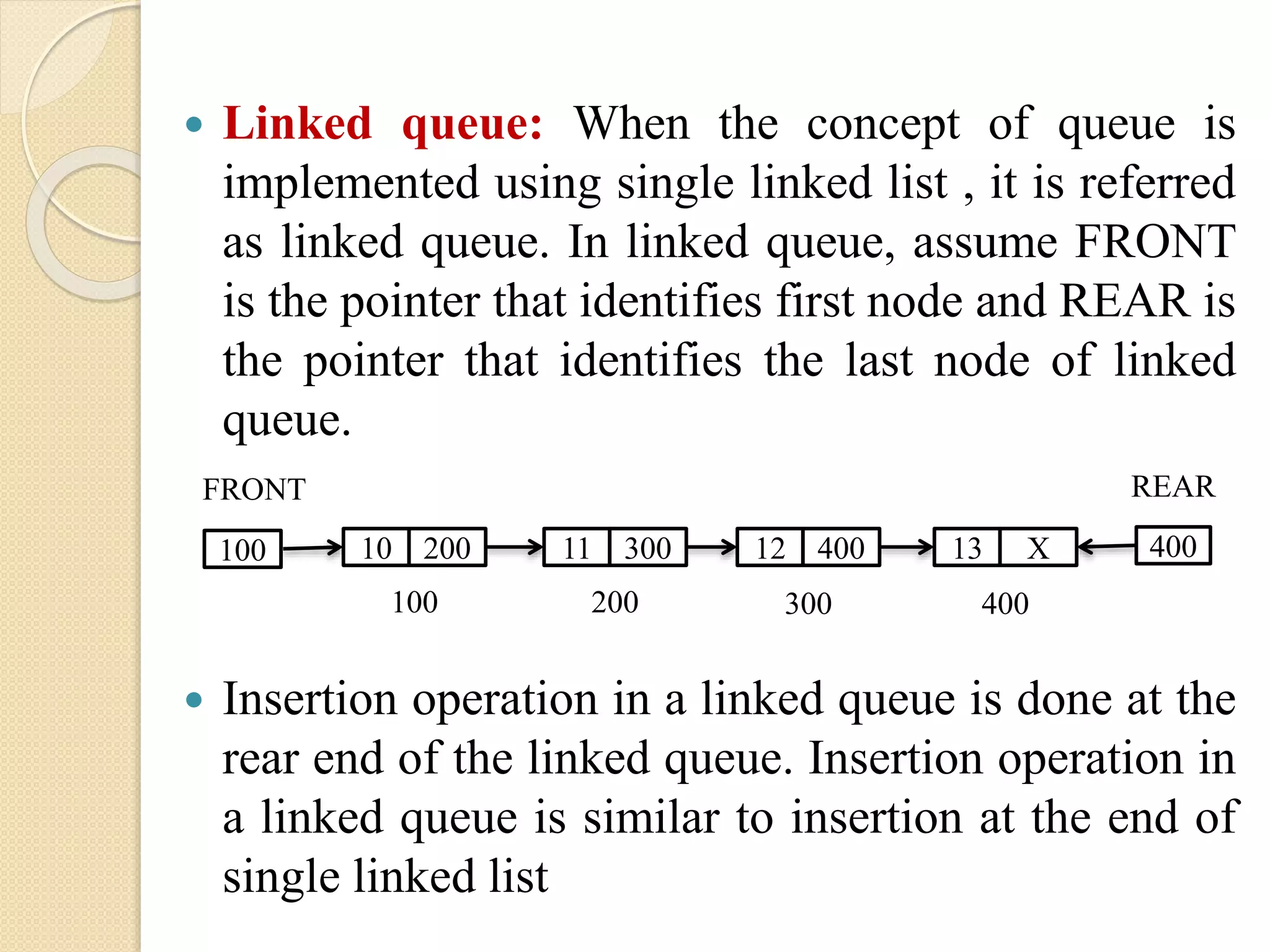
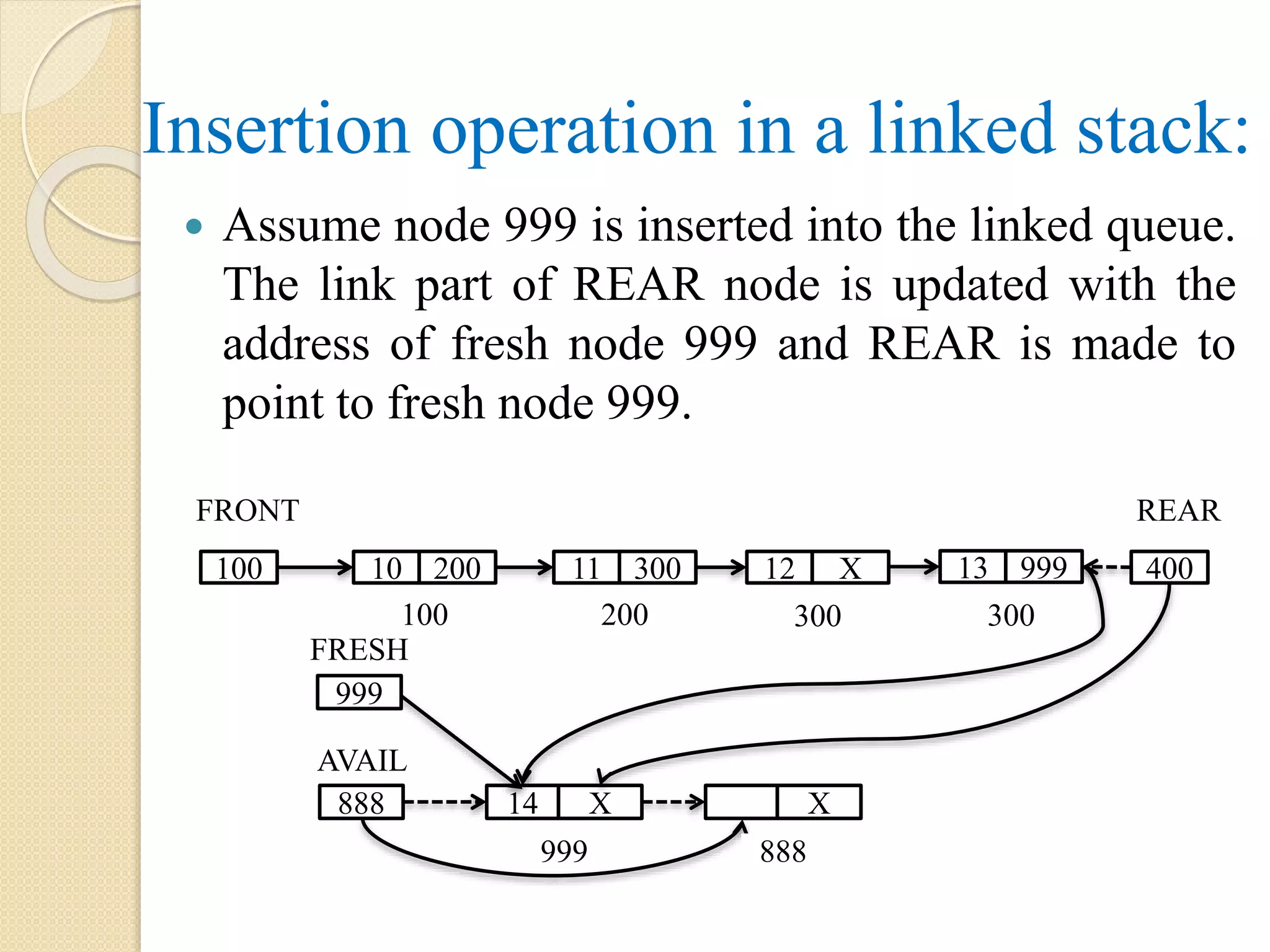
![Algorithm: LINKEDQUEUEINSERT(AVAIL, FRESH, LINK, FRONT, REAR, INFO, ITEM) Step 1: if AVAIL = NULL, then Display “Overflow” Step 2: else FRESH = AVAIL AVAIL = LINK[AVAIL] LINK[FRESH] = NULL INFO[FRESH] = ITEM](https://image.slidesharecdn.com/datastructureusingcmodule1-170525065731/75/Data-structure-using-c-module-1-201-2048.jpg)
![ Step 2.1: if FRONT = NULL AND REAR = NULL, then FRONT = FRESH REAR = FRESH Step 2.2: else LINK[REAR] = FRESH REAR = FRESH [End of if – Step 2.1] [End of if – Step 1] Step 3: Exit](https://image.slidesharecdn.com/datastructureusingcmodule1-170525065731/75/Data-structure-using-c-module-1-202-2048.jpg)

![Algorithm: LINKEDQUEUEDELETE(AVAIL, LINK, PTR, FRONT, REAR) Step 1: if FRONT = NULL AND REAR = NULL, then Display “Underflow” Step 2: else if FRONT = REAR, then FRESH = NULL REAR = NULL Step 3: else PTR = FRONT FRONT = LINK[FRONT] LINK[PTR] = AVAIL AVAIL = PTR [End of if] Step 4: Exit](https://image.slidesharecdn.com/datastructureusingcmodule1-170525065731/75/Data-structure-using-c-module-1-204-2048.jpg)
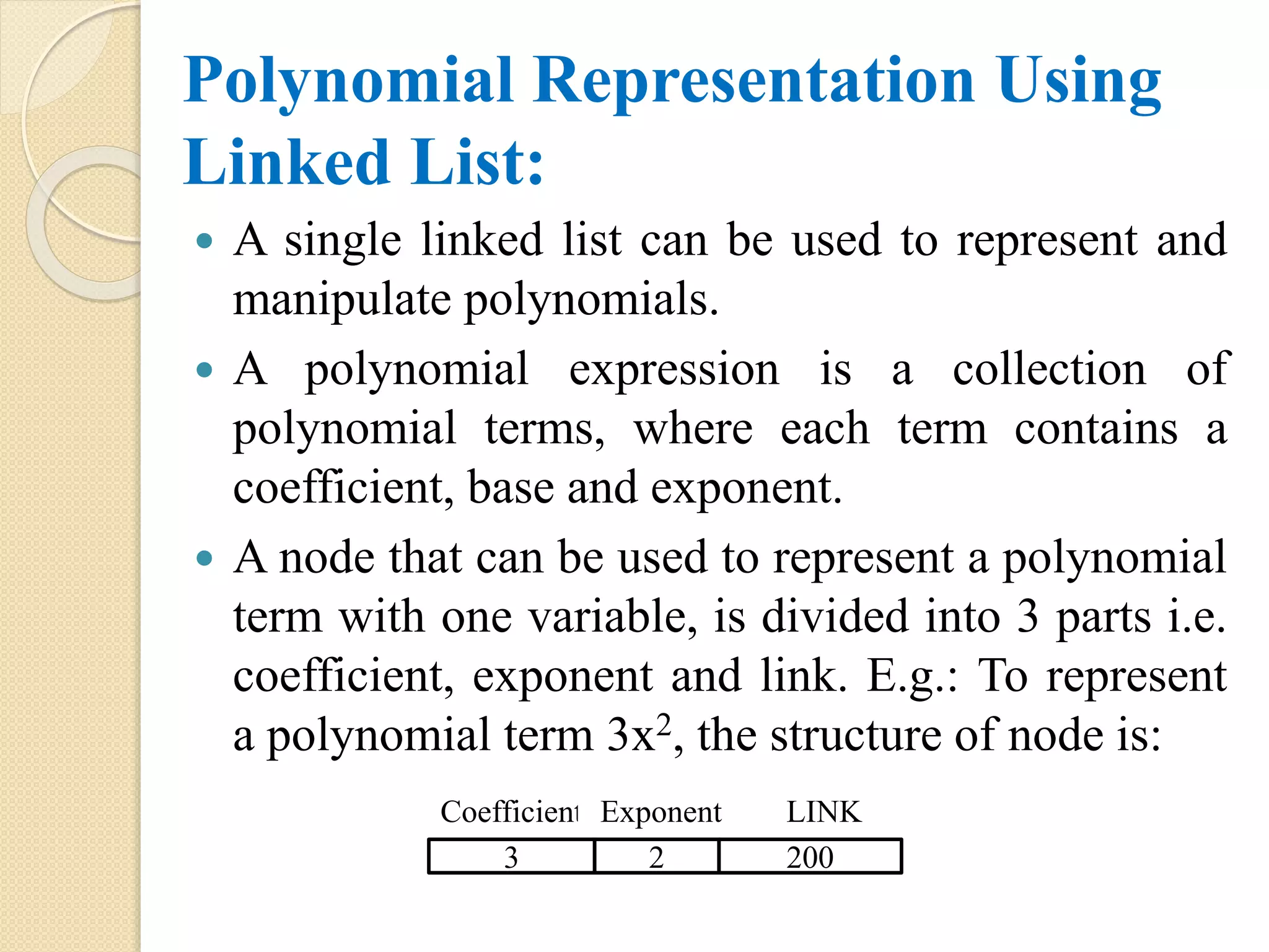
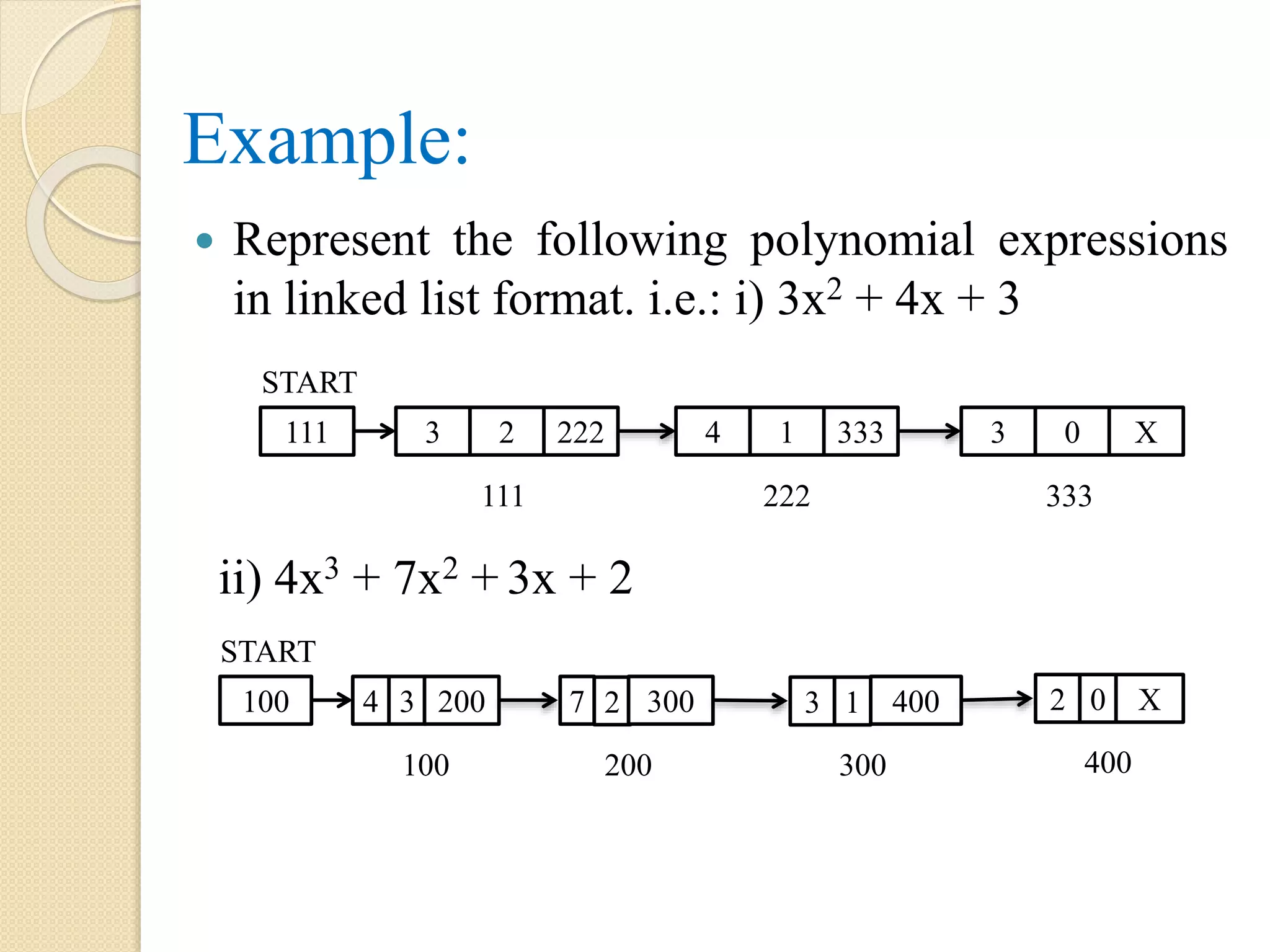
![Creating a polynomial using linked list: Algorithm: Create_Poly(START, AVAIL, CO, EXP, LINK, FRESH, PTR, PTR1) Step 1: if AVAIL = NULL, then Display “Memory Insufficient”. Step 2: else FRESH = AVAIL AVAIL = LINK[AVAIL] LINK[FRESH] = NULL Display “enter co-efficient and exponent values” Step 2.1: if START = NULL, then START = FRESH Step 2.2: else PTR1 = START](https://image.slidesharecdn.com/datastructureusingcmodule1-170525065731/75/Data-structure-using-c-module-1-207-2048.jpg)
![ Step 2.2.1: Repeat while PTR1! = NULL if EXP[PTR1] < EXP[FRESH], then break [End of if] PTR = PTR1 PTR1 = LINK[PTR1] [End of while] Step 2.2.2: if PTR1 = START, then LINK[FRESH] = PTR1 START = FRESH](https://image.slidesharecdn.com/datastructureusingcmodule1-170525065731/75/Data-structure-using-c-module-1-208-2048.jpg)
![ Step 2.2.3: else if PTR1 = NULL, then LINK[PTR] = FRESH Step 2.2.4: else LINK[PTR] = FRESH LINK[FRESH] = PTR1 [End of if – Step – 2.2.2] [End of if – Step 2.1] Step 3: Exit](https://image.slidesharecdn.com/datastructureusingcmodule1-170525065731/75/Data-structure-using-c-module-1-209-2048.jpg)
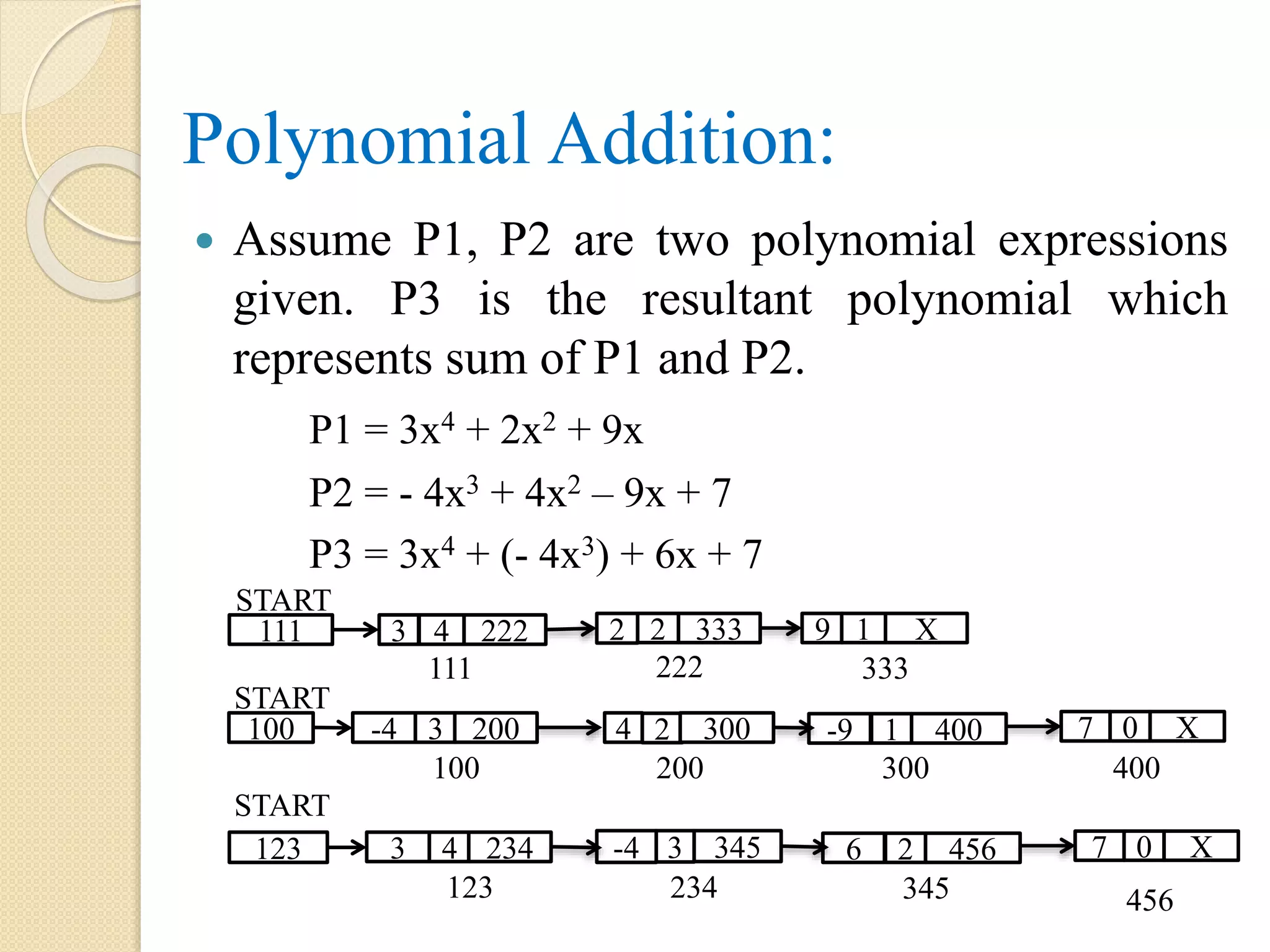
![Procedure for addition of two polynomials: [Assume P1 and P2 are two polynomials expressions and P3 is the resultant polynomial] Step 1: Repeat while P1 and P2 are NOT NULL, Repeat Step 2, 3 and 4 Step 2: if exponent parts of two terms of P1 and P2 are equal and if the co-efficient terms do not cancel to 0, then Step 2.1: Find sum of the co-efficient terms and insert SUM polynomial P3. Step 2.2: Move to next term of P1 Step 2.3: Move to next term of P2.](https://image.slidesharecdn.com/datastructureusingcmodule1-170525065731/75/Data-structure-using-c-module-1-211-2048.jpg)
![ Step 3: else if the exponent of the term in first polynomial > exponent of the term in second polynomial, then insert the term from first polynomial in the SUM polynomial. Step 3.1: Move to next term of P1. Step 4: else Step 4.1: Insert the term from the 2nd polynomial into SUM polynomial Step 4.2: Move to Next term of P2. [End of if] Step 5: Copy remaining terms from the non-empty polynomials into the SUM polynomial Step 6: Exit.](https://image.slidesharecdn.com/datastructureusingcmodule1-170525065731/75/Data-structure-using-c-module-1-212-2048.jpg)
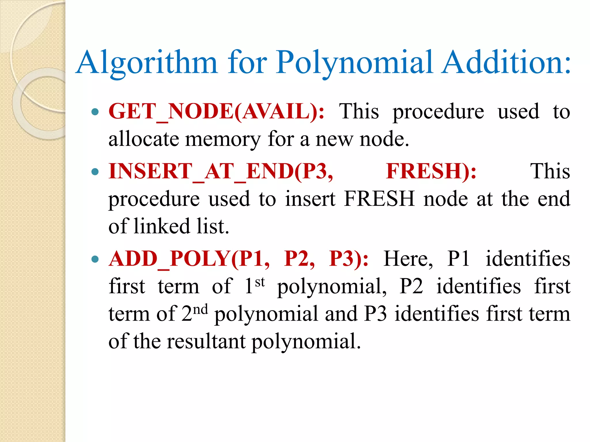
![GET_NODE(AVAIL) Step 1: Let PTR Step 2: if AVAIL = NULL, then Display “Overflow” Step 3: else PTR = AVAIL AVAIL = LINK[AVAIL] LINK[PTR] = NULL [End of if] Step 4: RETURN(PTR) Step 5: Exit](https://image.slidesharecdn.com/datastructureusingcmodule1-170525065731/75/Data-structure-using-c-module-1-214-2048.jpg)
![INSERT_AT_END(P3, FRESH) Step 1: Let PTR Step 2: if P3 = NULL, then P3 = FRESH Step 3: else Step 3.1: Set PTR = P3 Step 3.2: Repeat while (LINK[PTR] != NULL) PTR = LINK[PTR] [End of while] Step 3.3: LINK[PTR] = FRESH Step 4: Exit](https://image.slidesharecdn.com/datastructureusingcmodule1-170525065731/75/Data-structure-using-c-module-1-215-2048.jpg)
![ADD_POLY(P1, P2, P3) Step 1: Let PTR1, PTR2, FRESH Step 2: P3 = NULL Step 3: PTR1 = P1 Step 4: PTR2 = P2 Step 5: Repeat while (PTR1 != NULL AND PTR2 != NULL) Step 5.1: if EXP[PTR1] > EXP[PTR2], then FRESH = GET_NODE(AVAIL) EXP[FRESH] = EXP[PTR1] CO[FRESH] = CO[PTR1] INSERT_AT_END(P3, FRESH) PTR1 = LINK[PTR1]](https://image.slidesharecdn.com/datastructureusingcmodule1-170525065731/75/Data-structure-using-c-module-1-216-2048.jpg)
![ Step 5.2: else if EXP[PTR2] > EXP[PTR1], then FRESH = GET_NODE(AVAIL) EXP[FRESH] = EXP[PTR2] CO[FRESH] = CO[PTR2] INSERT_AT_END(P3, FRESH) PTR2 = LINK[PTR2] Step 5.3: else FRESH = GET_NODE(AVAIL) EXP[FRESH] = EXP[PTR1] CO[FRESH] = CO[PTR1] + CO[PTR2] Step 5.3.1: if CO[FRESH] = 0, then INSERT_AT_END(P3, FRESH) [End of if – Step 5.3.1]](https://image.slidesharecdn.com/datastructureusingcmodule1-170525065731/75/Data-structure-using-c-module-1-217-2048.jpg)
![PTR1 = LINK[PTR2] PTR2 = LINK[PTR2] [End of if – Step 5.1] [End of while – Step 5] Step 6: Repeat while PTR2 != NULL FRESH = GET_NODE(AVAIL) EXP[FRESH] = EXP[PTR2] CO[FRESH] = CO[PTR2] INSERT_AT_END(P3, FRESH) PTR2 = LINK[PTR2] [End of while – Step 6]](https://image.slidesharecdn.com/datastructureusingcmodule1-170525065731/75/Data-structure-using-c-module-1-218-2048.jpg)
![ Step 7: Repeat while PTR1 != NULL FRESH = GET_NODE(AVAIL) EXP[FRESH] = EXP[PTR1] CO[FRESH] = CO[PTR1] INSERT_AT_END(P3, FRESH) PTR1 = LINK[PTR1] [End of while – Step 7] Step 8: RETURN(P3) Step 9: Exit](https://image.slidesharecdn.com/datastructureusingcmodule1-170525065731/75/Data-structure-using-c-module-1-219-2048.jpg)