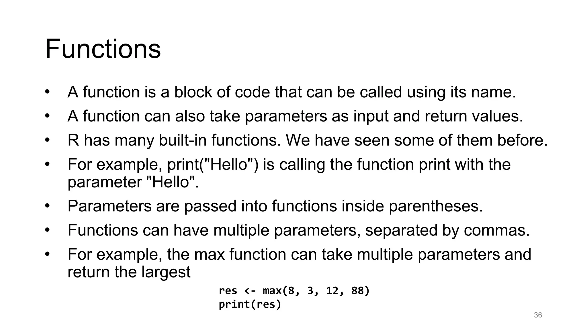
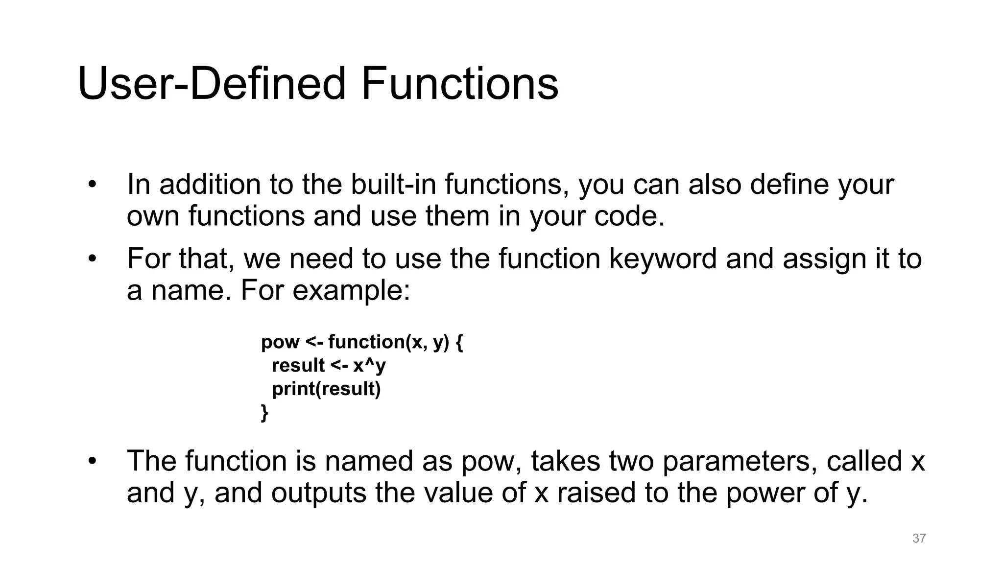
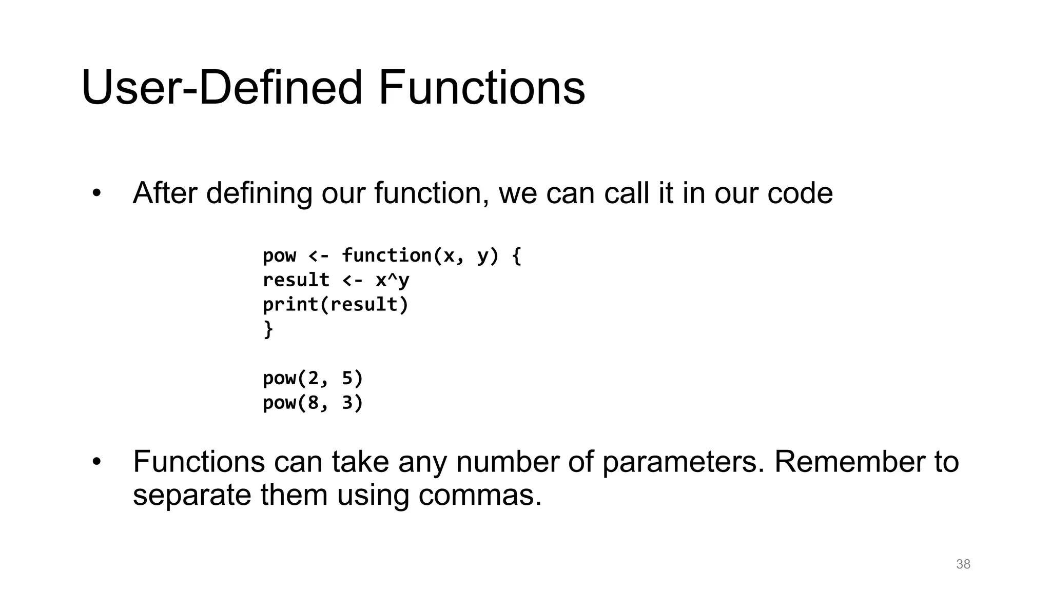
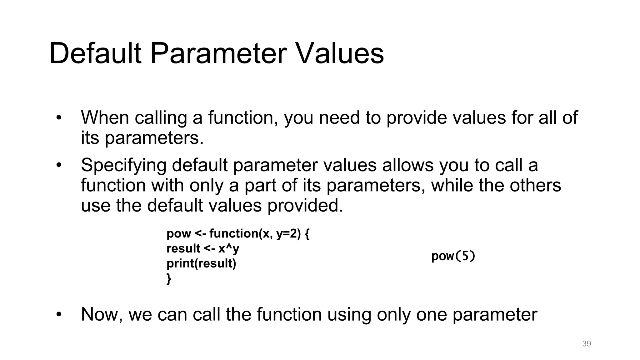
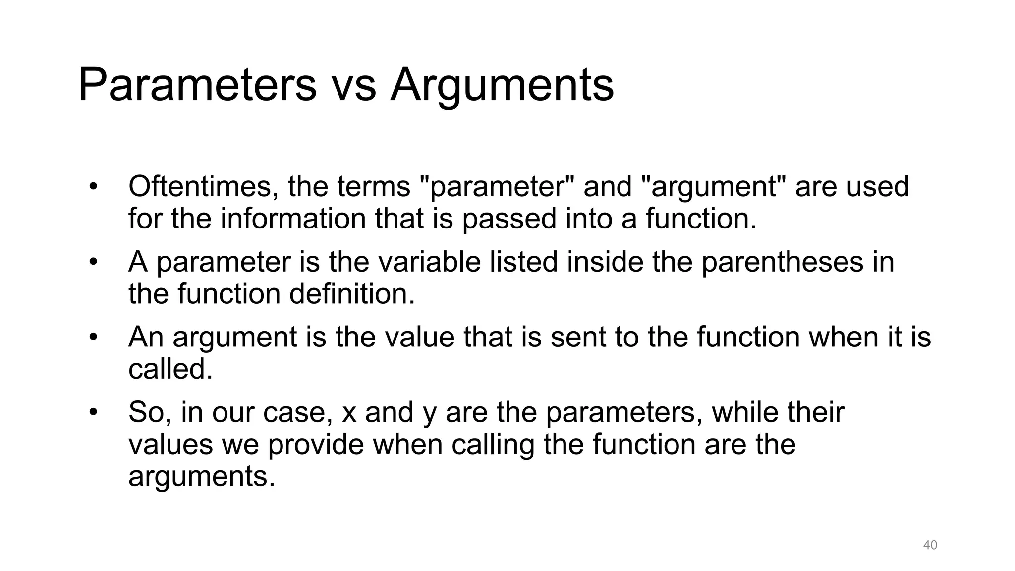
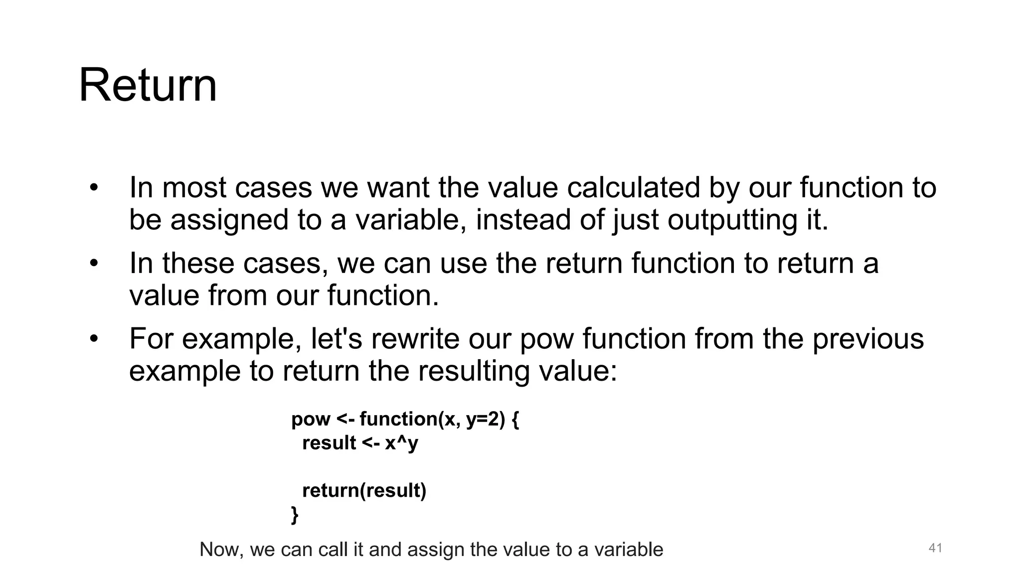
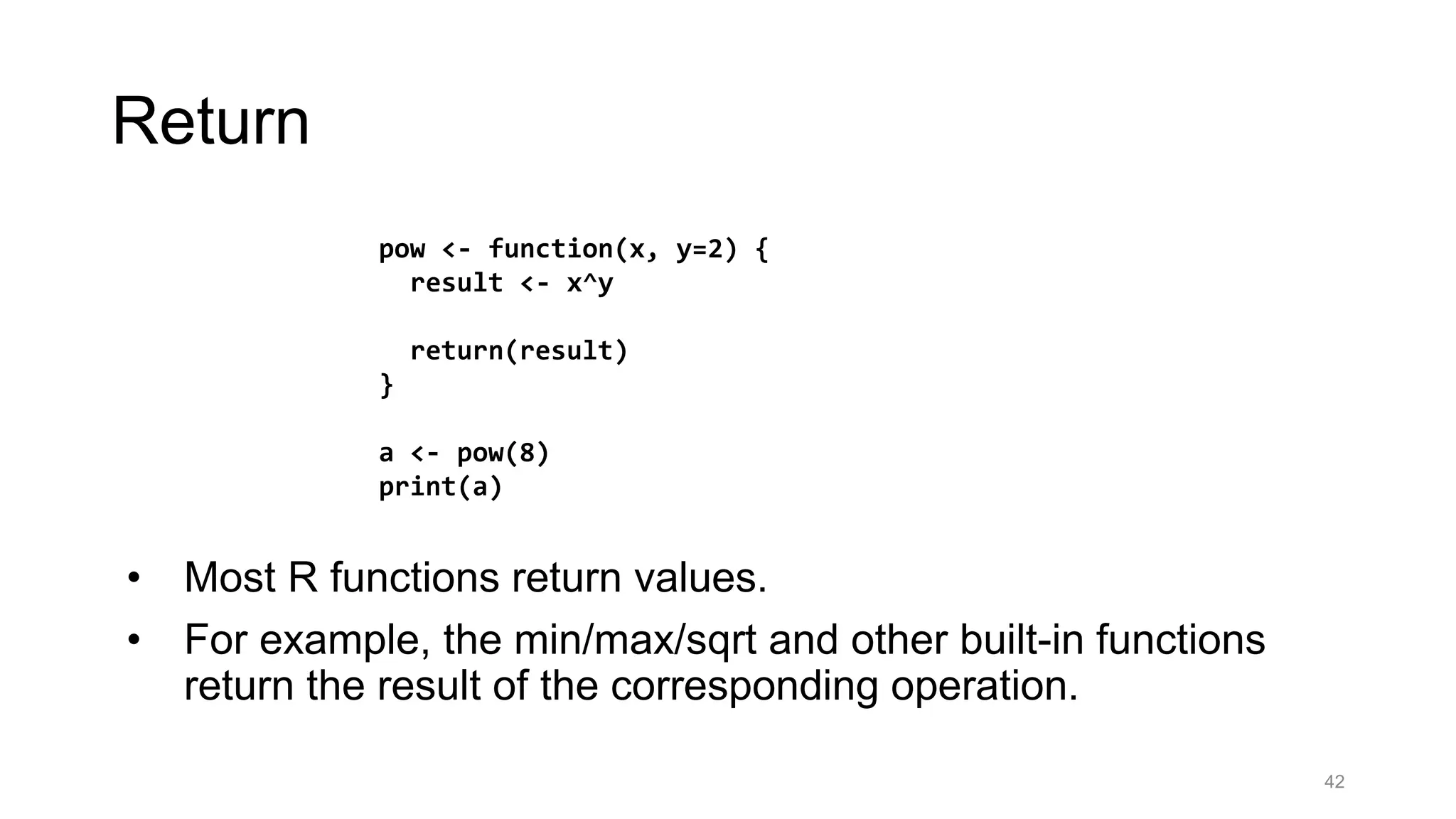
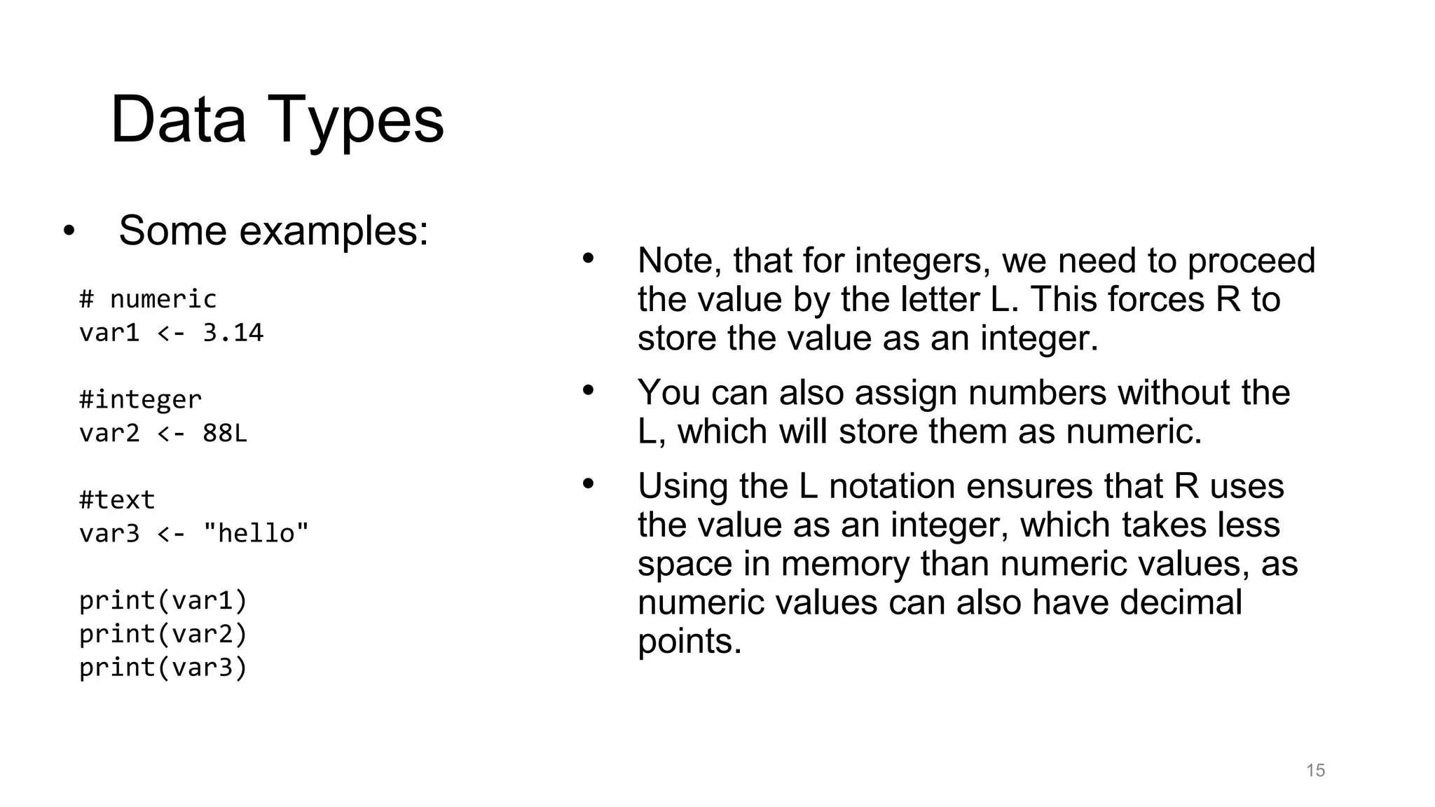
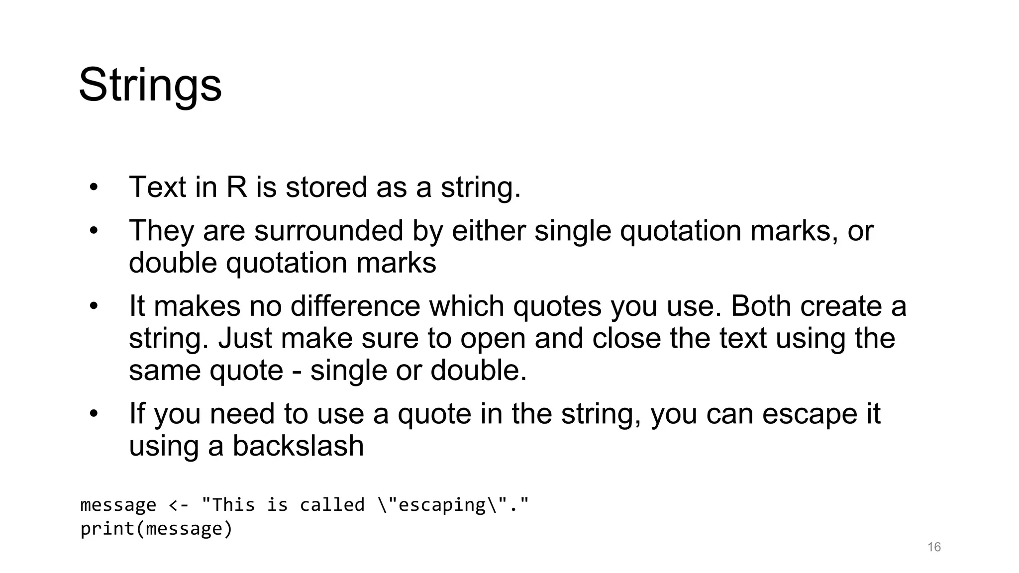
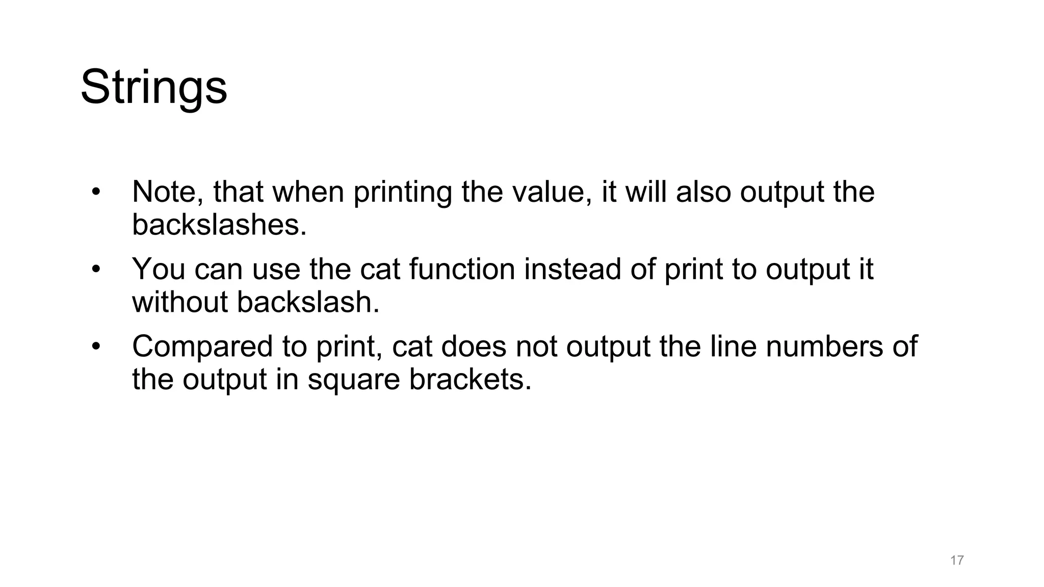
data analysis using R programming language

Getting Started with R Yusuf Ibrahim

What is R? RStudio? • R – a programming language + software that interprets it • RStudio – popular software to write R scripts and interact with the R software 2

R • R is among the most extensively employed statistical programming languages and is the foremost preference of data experts and analysts. • Throughout this course, we shall gain knowledge of the fundamental principles of R • learn how to create programs that store & manipulate data • perform data analysis tasks using various data sets • visualize the results using graphs and charts 3

What R is and what it is not • R is • a programming language • a statistical package • an interpreter • Open Source • R is not • a database • a collection of “black boxes” • a spreadsheet software package • commercially supported

Setup Instructions • Install R and RStudio now if you have not already done so https://cran.r-project.org/ https://posit.co/download/rstudio-desktop/ 5

Create a new R script • File > New File > R Script • Save it in your scripts folder 6

R Studio Interface Script Console Environment Files 7

Script vs console • Both accept commands • Console: runs the commands • Enter to run • Script: saves your code • Ctrl/Cmd+enter to run WRITE RUN Ctrl-Enter 8

First Program • Let's start by writing a simple program that outputs text. • The print function is used to output text. • It is followed by parentheses, which include the text we want to output, enclosed in quotes. • Note, that the output also includes a number before it: that is the line number of the output. 9 print(“Hello World!") [1] "Learning R is fun!" output

Comments • Comments are used to explain your code. They are ignored when your program is run. • You can create comments in R using #. For example: • Anything that comes after the # symbol on that line is ignored! • Comments are useful, as they help to read and understand larger segments of code, and explain what the code is doing. 10 #outputs "Hello, World!" print("Hello, World!") [1] "Hello, World!" output

Variables • Generally, every R program deals with data. • Variables allow you to store and manipulate data. Variables have a name and a value. • For example, let's create a variable named x and store the value 42 in it: • Note, that we used the assignment operator = to assign a value to the variable. • Now, we can use print to output the value stored in x: • Variable names have to start with a letter or a dot and can include letters, numbers and a dot or underline characters. 11 x = 42 x = 42 print(x) [1] 42 output

Variables • A more preferred way of assigning values to variables in R is using the leftward <- operator: • We can have multiple variables in our program, use different values for them and assign them new values during our program. 12 x <- 42 print(x) [1] 42 output

Variables • We can have multiple variables in our program, use different values for them and assign them new values during our program. For example: • R is case-sensitive, so, for example, Price and price are two different variables. 13 price <- 99.9 name <- “Yusuf" message <- "Some text" price <- 42.6 print(price) print(name) output [1] 42.6 [1] "Yusuf"

Data Types • Variables can store different types of data, such as integers, decimals, text. • In R, you do not need to specify the type a variable will hold. Instead, R will automatically get the type from the value it is assigned to. • Some examples: 14

Data Types • Some examples: • Note, that for integers, we need to proceed the value by the letter L. This forces R to store the value as an integer. • You can also assign numbers without the L, which will store them as numeric. • Using the L notation ensures that R uses the value as an integer, which takes less space in memory than numeric values, as numeric values can also have decimal points. 15 # numeric var1 <- 3.14 #integer var2 <- 88L #text var3 <- "hello" print(var1) print(var2) print(var3)

Strings • Text in R is stored as a string. • They are surrounded by either single quotation marks, or double quotation marks • It makes no difference which quotes you use. Both create a string. Just make sure to open and close the text using the same quote - single or double. • If you need to use a quote in the string, you can escape it using a backslash 16 message <- "This is called "escaping"." print(message)

Strings • Note, that when printing the value, it will also output the backslashes. • You can use the cat function instead of print to output it without backslash. • Compared to print, cat does not output the line numbers of the output in square brackets. 17

Arithmetic Operators • R supports basic arithmetic operations. • You can use them for variables or values. • Note, that R supports two types of division • division and integer division. • The first version produces a decimal, while the second one produces a whole number. 18 # Examples x <- 11 y <- 4 #addition print(x+y) #substraction print(x-y) #multiplication print(x*y) #division print(x/y) #exponentation print(x^y) #or x**y #modulus (remainder from division) print(x%%y) #integer division print(x%/%y)

Math Functions • R also supports functions to perform mathematical tasks. • For example, the min and max functions can be used to find the minimum and maximum of a given set of numbers • You can also use more than 2 numbers with the min and max functions • just separate them using commas. 19 a <- 8 b <- 12 #minimum print(min(a, b)) #maximum print(max(a, b))

• Similarly, R has a built-in sqrt function, that is used to find the square root of a given number • Remember, that you need to use parentheses to enclose the numbers in the functions. 20 print(sqrt(64))

Booleans • Boolean is another data type in R. • It can have one of the following 2 values: TRUE and FALSE. • Booleans are created when we compare values. • For example: • In the code above, we used the greater than > operator to compare x with the value 20. • The result of the comparison is a Boolean with the value FALSE, as x is not greater than 20. 21 x <- 14 print(x > 20)

Relational Operators • R supports the following relational operators, used for comparisons: • > greater than; • < less than; • <= less than or equal to; • >= greater than or equal to; • == equal • != not equal 22 Note, that you need to use two equal signs for checking for equality, as a single equal sign is the assignment operator. x <- 42 print(x >= 8) print(x < 24) print(x == 42) print(x != 42)

Output • As we have seen in the previous lessons, we can output values using the print and the cat functions. • You can use the n special symbol to add new lines to text. • You can have multiple n symbols in your text. • Note that the cat function shows the line break in the output, while the print function shows the n character without the line break. 23 x <- "hello" print(x) cat(x) x <- "hellonthere!" print(x) cat(x)

Decision Making • In many situations, you need to make a decision based on a condition. • For that, you can use the if statement. • For example: • As you can see, the if keyword is followed by the condition in parentheses and a code block in curly braces, which gets executed if the condition is TRUE. • In case the condition of the if statement is FALSE, the code in the curly braces will not run. 24 x <- 24 if(x > 10) { print("x is greater than 10") }

Else • In case you need to run code when the condition of an if statement is FALSE, you can use an else statement 25 x <- 42 if(x >= 100) { print("x is big") } else { print("x is less than 100") }

multiple else if • In case you need multiple checks, you can use multiple else if statements. • For example, let's output the English version of the given number: • You can have as many else if statements as you want. 26 num <- 3 if(num == 1) { print("One") } else if(num == 2) { print("Two") } else if (num == 3) { print("Three") } else { print("Something else") }

Logical Operators • Logical operators allow you to combine multiple conditions. • The logical & (AND) operator allows you to combine two conditions and returns TRUE only if both conditions are TRUE. • For example: 27 x <- 6 y <- 2 if(x>y & x < 10) { print("Yes") }

Logical Operators • Similarly, the logical | (OR) operator returns TRUE if any one of its conditions is TRUE: • The logical ! (NOT) operator returns the opposite of the given condition: • You can combine multiple conditions using the logical operators and group conditions using parentheses, just like mathematical operations. 28 x <- 6 y <- 2 if(x>y | x > 100) { print("Yes") } x <- TRUE print(!x)

Switch (using index) • R provides a switch statement to test an expression against a list of values and makes the code much shorter, compared to using else if statements. • Let's see it in action: 29 num <- 3 result <- switch( num, "One", "Two", "Three", "Four" ) print(result)

switch • The switch statement takes its first parameter and returns the value whose index corresponds to that number. • Instead of the index, you can also provide the values to compare and the values to return in case they match: 30 x <- "c" result <- switch( x, "a" = "One", "b" = "Two", "c" = "Three", "d" = "Four" ) print(result) You can have as many cases as you want. Just remember to separate them using commas.

Loops • Loops allow you to repeat a block of code until a given condition is TRUE. • The while loop has the following syntax: • Let's use it to output the numbers 1 to 9: 31 while (condition) { code to run } i <- 1 while (i < 10) { print(i) i <- i + 1 }

Loops • The code above checks if i is less than 10, outputs its value, and then increments it by 1. • This means that the loop will output the numbers 1 to 9 and stop when i reaches the value 10. • Each time the computer runs through a loop, it's referred to as an iteration. • It is important to change the condition's value during the iterations of the while loop, as not doing so will result in an infinite loop, because the condition will always remain TRUE. 32

For Loop • Another loop that R provides is the for loop. • It is used to iterate over a given sequence. • R allows us to create a sequence of numbers by using a colon and specifying the lower and upper bounds. • The sequence in the code above will include the numbers 1 to 10. • During each iteration of the for loop, the x variable will take the value of the next number in the sequence, thus, the resulting output will be the numbers 1 to 10. 33 for (x in 1:10) { print(x) } [1] 1 [1] 2 [1] 3 [1] 4 [1] 5 [1] 6 [1] 7 [1] 8 [1] 9 [1] 10

break • The break statement allows you to stop a loop. • For example: • The code above will stop the loop when i reaches the value 4. • This can be particularly useful when you need to take multiple inputs from the user and stop in case a specific input is given. 34 i <- 8 while(i > 0) { print(i) i <- i - 1 if(i == 4) { break } } The break statement can also be used with

next • The next statements allows you to skip an iteration and continue running the loop at the next iteration. • For example, let's say we want to output all the numbers from 1 to 15, except 13 • Note that we check for the condition for the next statement before printing the value. • Similar to the break statement, the next statement can be used with both while and for loops. 35 for(x in 1:15) { if(x == 13) { next } print(x) }

Functions • A function is a block of code that can be called using its name. • A function can also take parameters as input and return values. • R has many built-in functions. We have seen some of them before. • For example, print("Hello") is calling the function print with the parameter "Hello". • Parameters are passed into functions inside parentheses. • Functions can have multiple parameters, separated by commas. • For example, the max function can take multiple parameters and return the largest 36 res <- max(8, 3, 12, 88) print(res)

User-Defined Functions • In addition to the built-in functions, you can also define your own functions and use them in your code. • For that, we need to use the function keyword and assign it to a name. For example: • The function is named as pow, takes two parameters, called x and y, and outputs the value of x raised to the power of y. 37 pow <- function(x, y) { result <- x^y print(result) }

User-Defined Functions • After defining our function, we can call it in our code • Functions can take any number of parameters. Remember to separate them using commas. 38 pow <- function(x, y) { result <- x^y print(result) } pow(2, 5) pow(8, 3)

Default Parameter Values • When calling a function, you need to provide values for all of its parameters. • Specifying default parameter values allows you to call a function with only a part of its parameters, while the others use the default values provided. • Now, we can call the function using only one parameter 39 pow <- function(x, y=2) { result <- x^y print(result) } pow(5)

Parameters vs Arguments • Oftentimes, the terms "parameter" and "argument" are used for the information that is passed into a function. • A parameter is the variable listed inside the parentheses in the function definition. • An argument is the value that is sent to the function when it is called. • So, in our case, x and y are the parameters, while their values we provide when calling the function are the arguments. 40

Return • In most cases we want the value calculated by our function to be assigned to a variable, instead of just outputting it. • In these cases, we can use the return function to return a value from our function. • For example, let's rewrite our pow function from the previous example to return the resulting value: 41 pow <- function(x, y=2) { result <- x^y return(result) } Now, we can call it and assign the value to a variable

Return • Most R functions return values. • For example, the min/max/sqrt and other built-in functions return the result of the corresponding operation. 42 pow <- function(x, y=2) { result <- x^y return(result) } a <- pow(8) print(a)

data analysis using R programming language

More Related Content

Similar to data analysis using R programming language

Recently uploaded

data analysis using R programming language