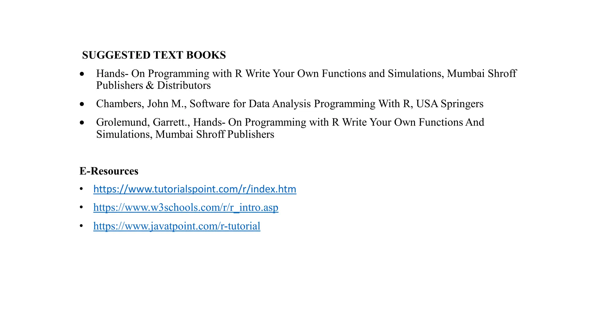
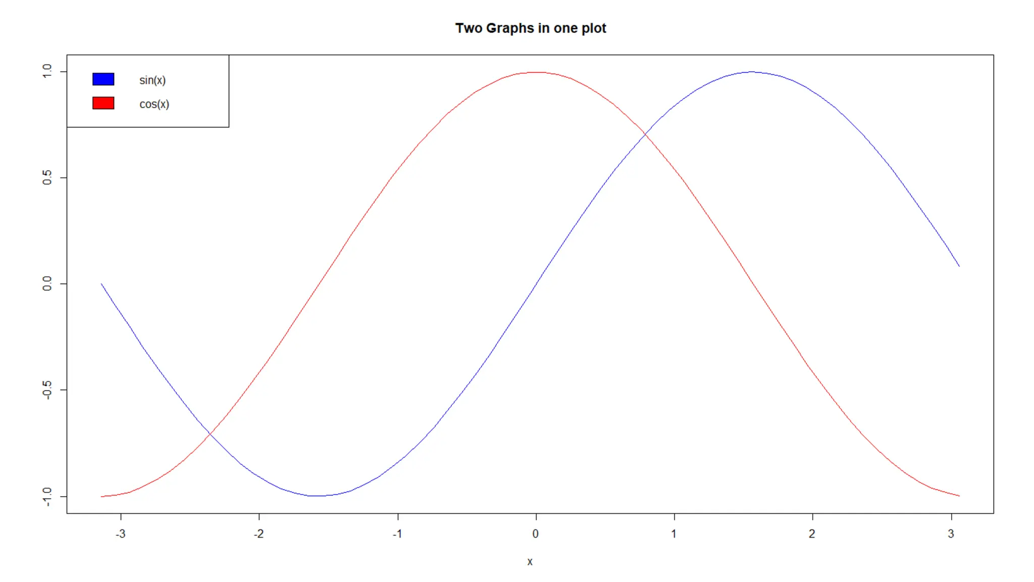
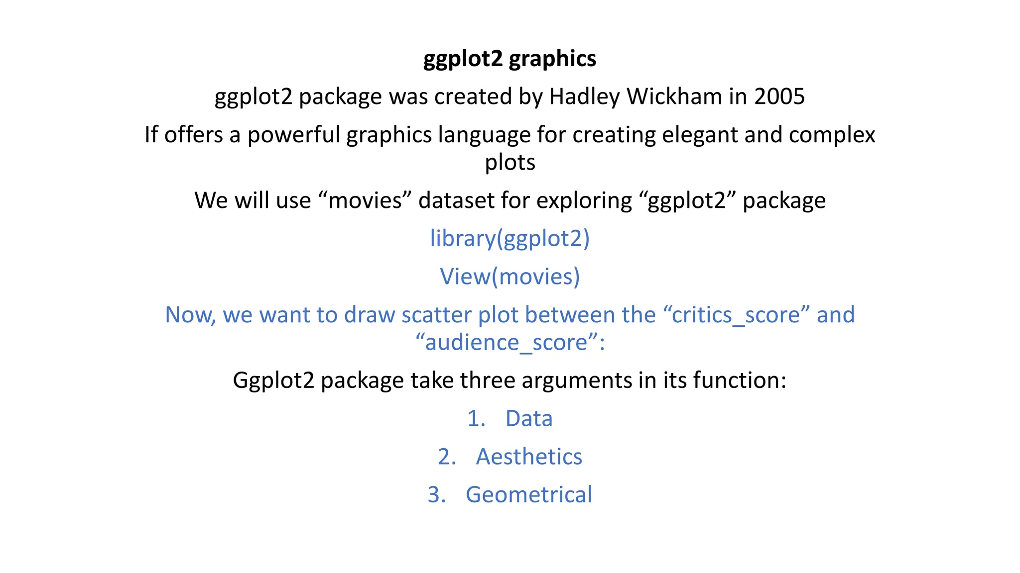
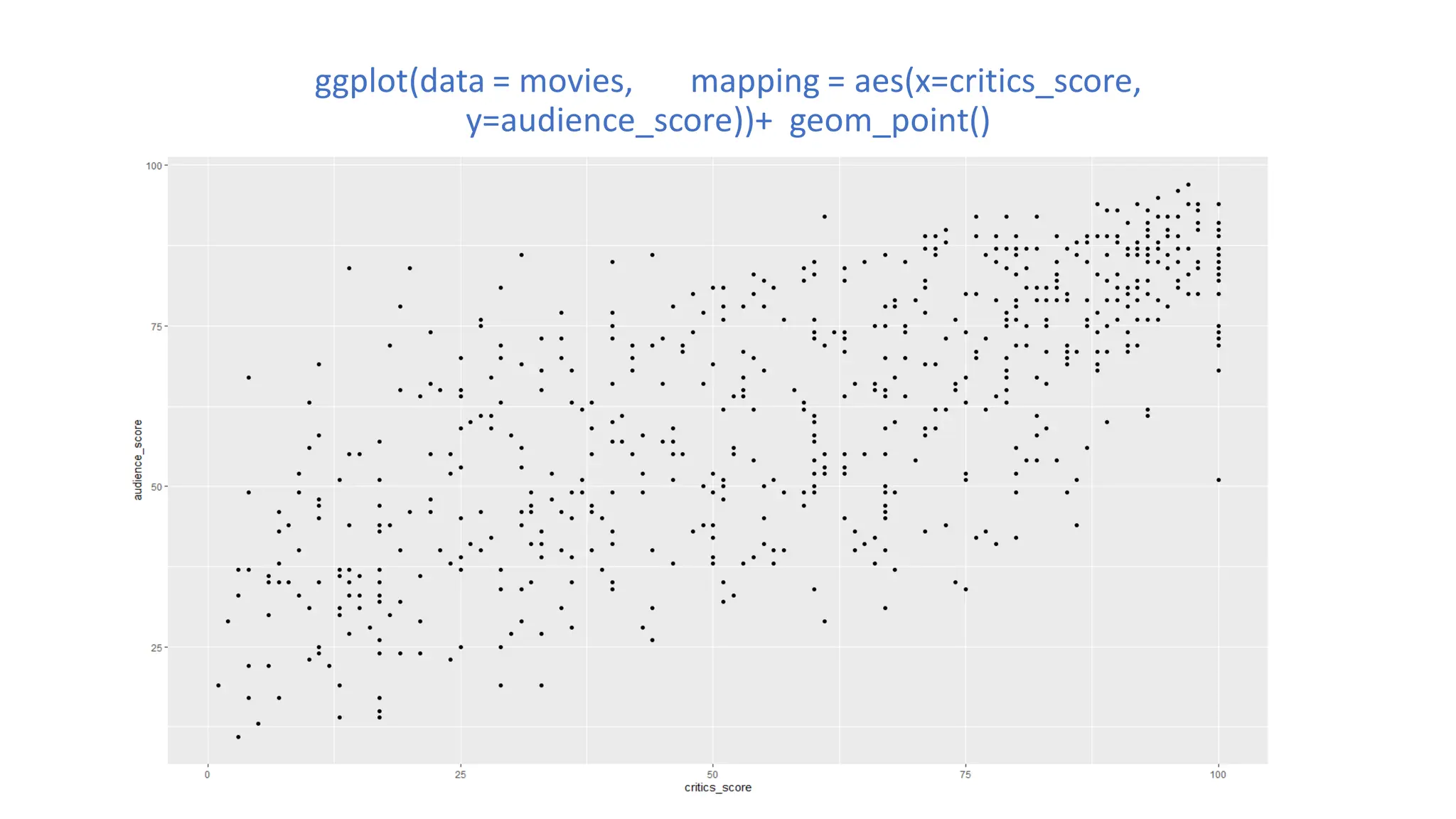
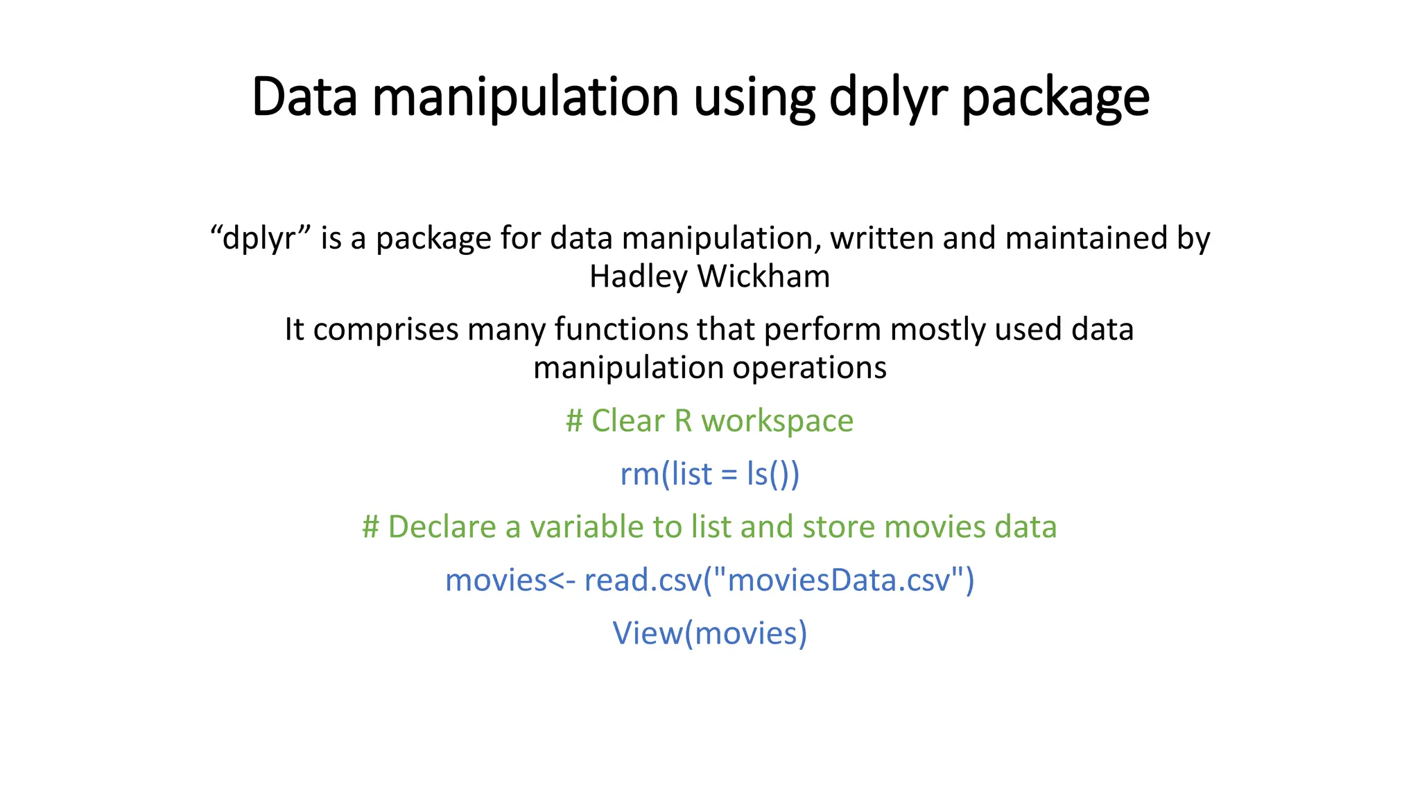
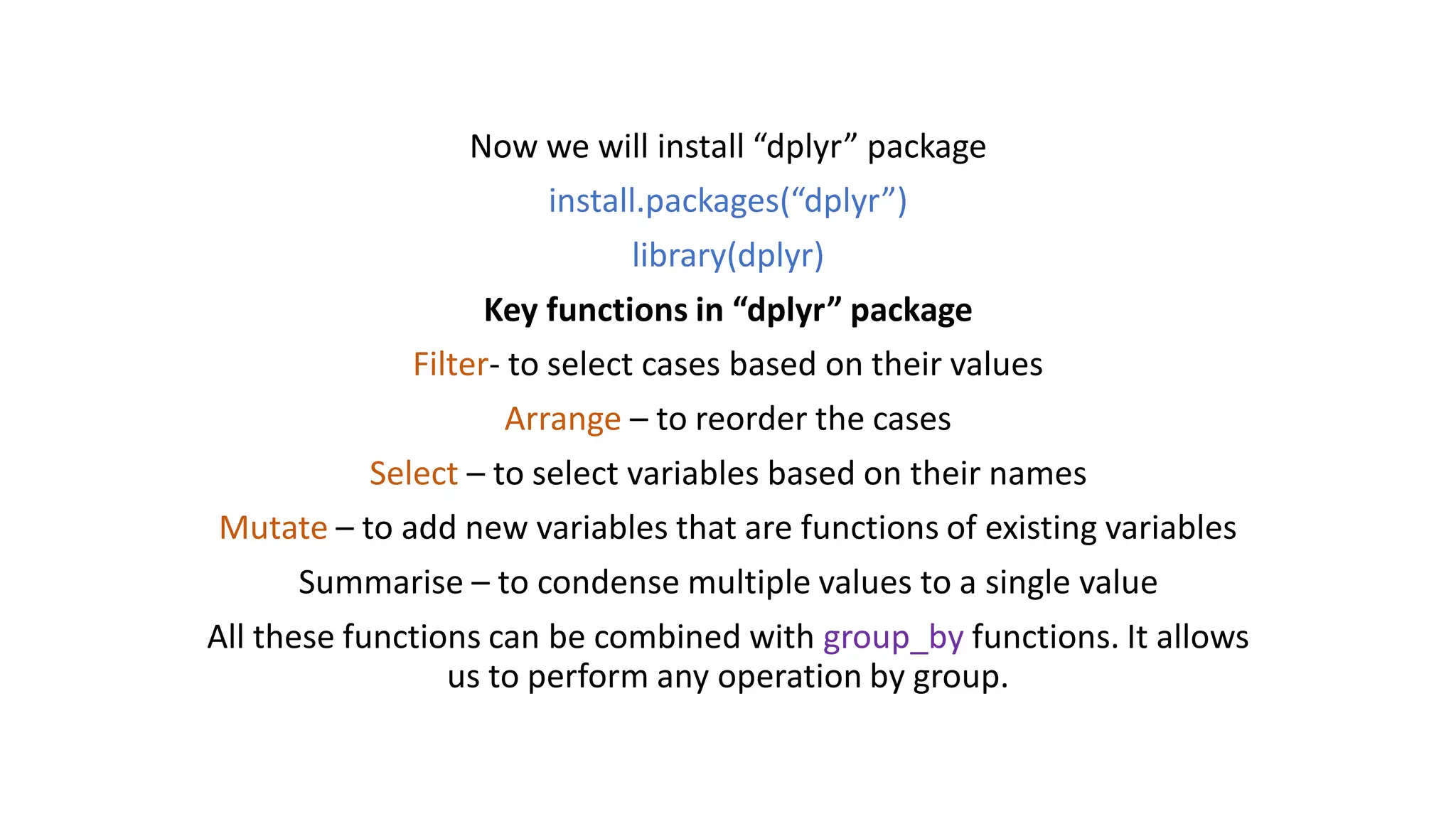
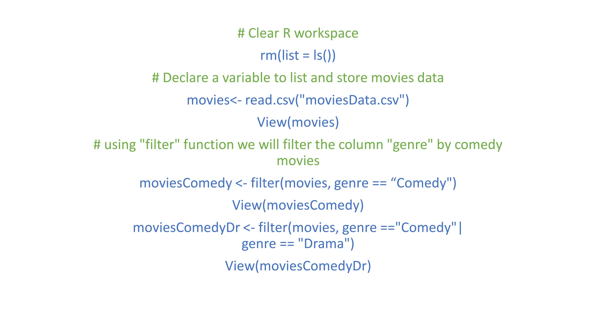
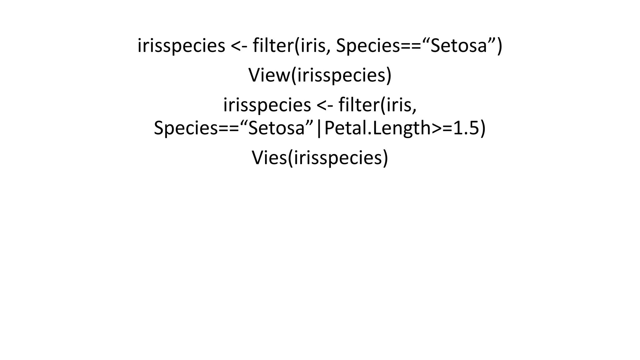
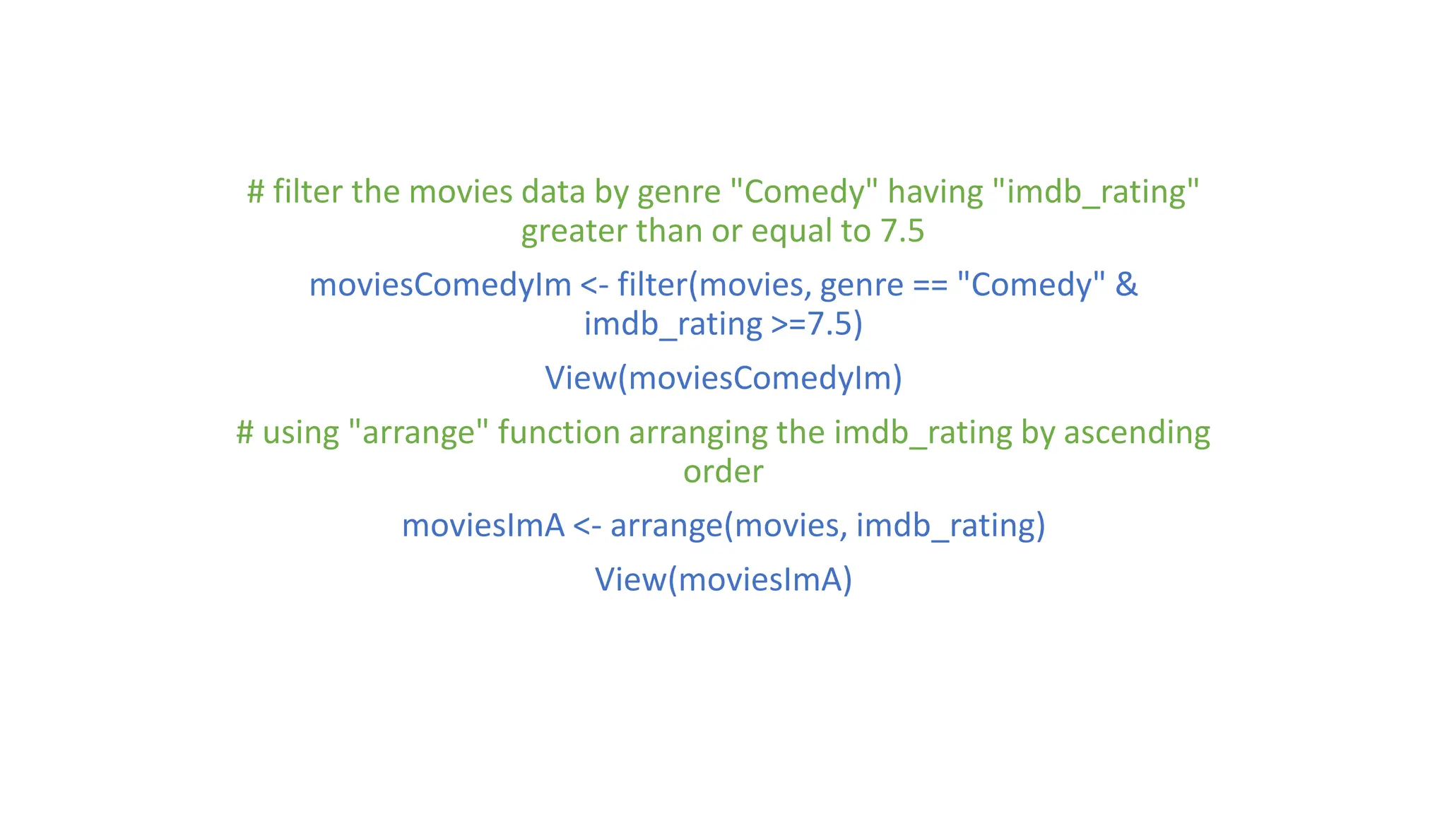
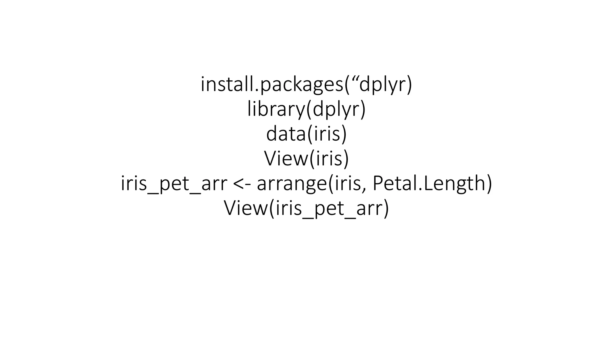
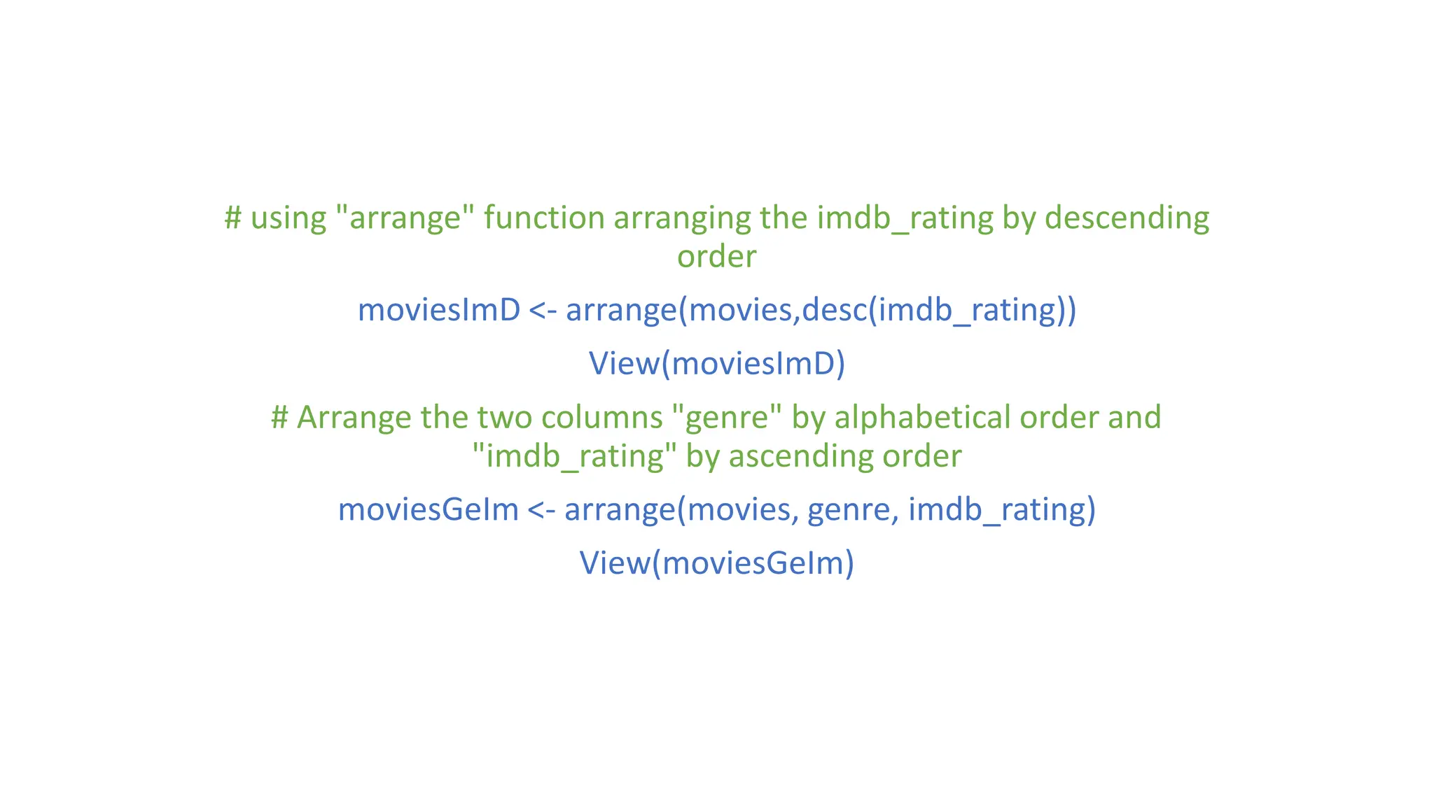
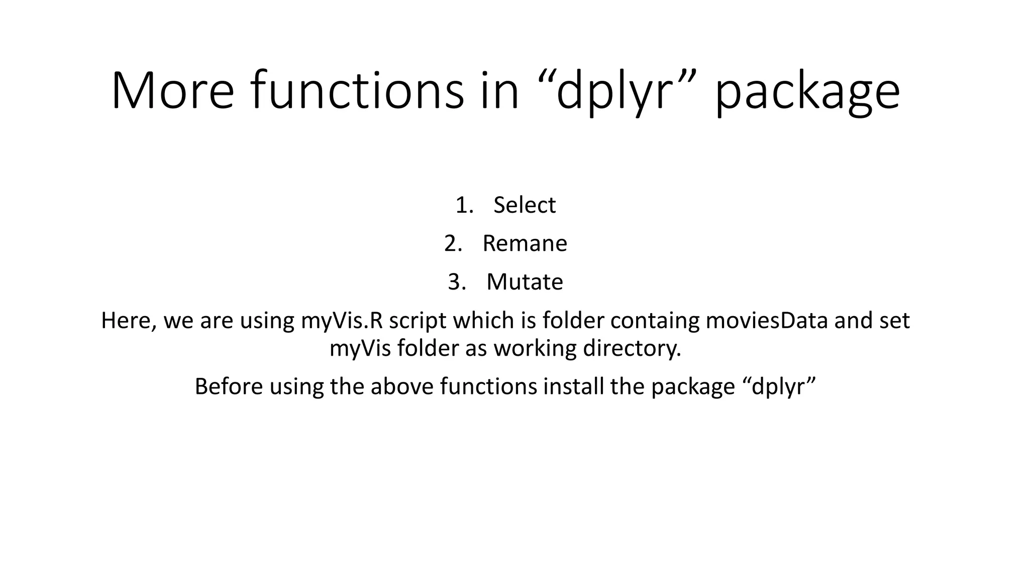
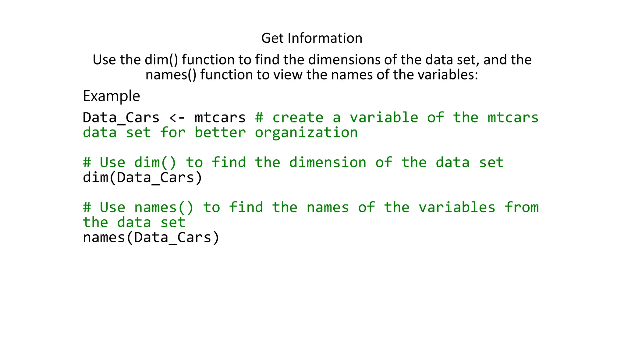
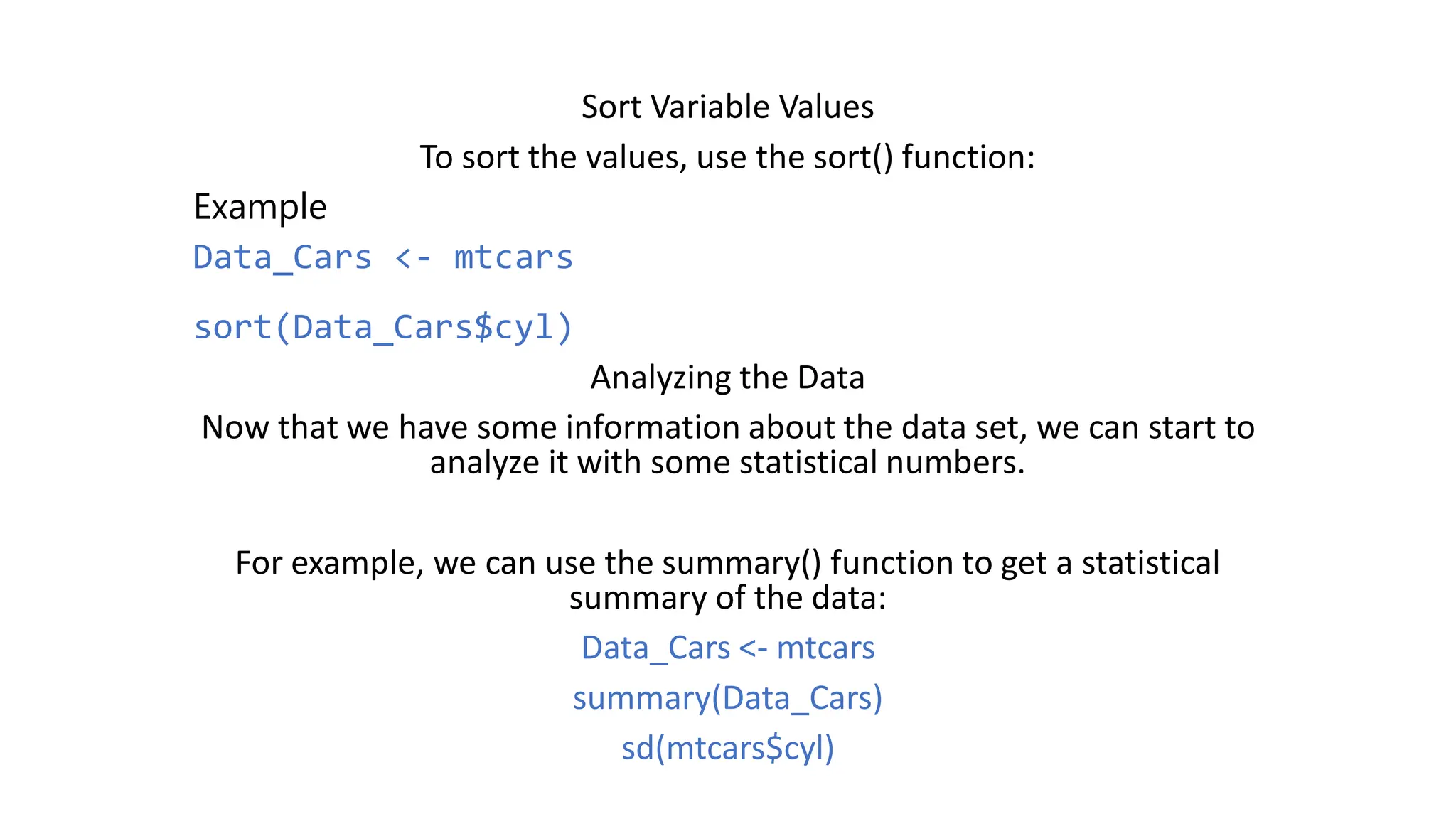
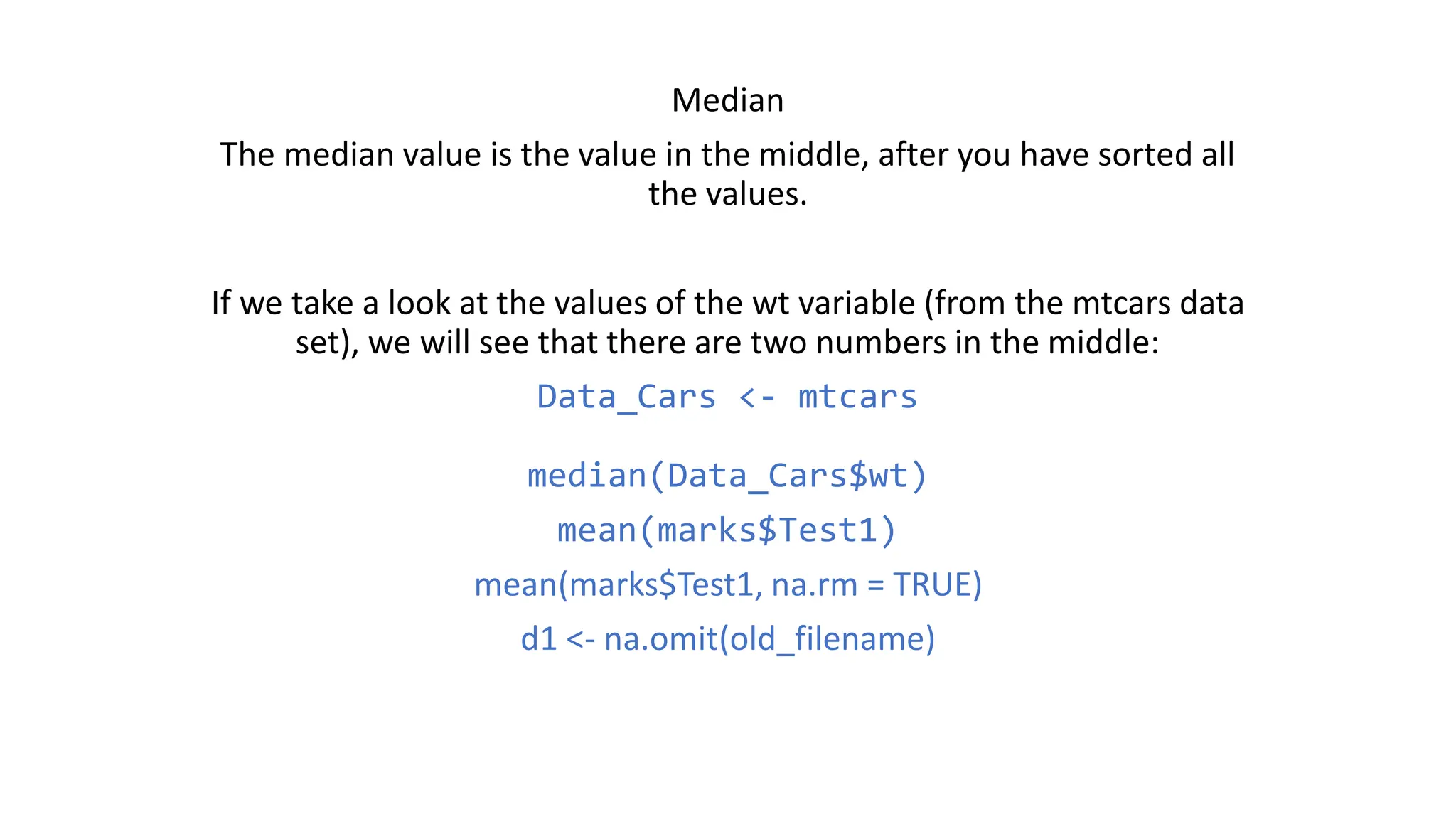
This document serves as an introductory guide to R programming for analytics, discussing its capabilities, benefits, and installation methods. It covers essential topics such as using R with integrated development environments (IDEs), managing data frames, and implementing statistical techniques and visualizations. The document also provides examples of functions and packages, as well as recommendations for textbooks and e-resources.
![Obtaining additional R Packages For Working with R you will need additional packages These packages are combination of data and functions The packages are kept in package repositories To Use packages you will have to install and then call them Installing: use install.packages(“name of the package”, repos = “”, dep = T) To Use Packages, use library(name of the package), also require(name of the package) [Use either]](https://image.slidesharecdn.com/basicsofrprogrammingforanalyticsautosaved1-240916080545-0682f8c8/75/Basics-of-R-programming-for-analytics-Autosaved-1-pdf-6-2048.jpg)
![What can we put in [>] and take out [<] from R? From Spreadsheets [ > ] Source Code Files [ > ] From other Software [ > ] Text Based Data [ > ] [ < ] Tables of Data [ > ] [ < ] Images [ < ] Dump Files [ < ]](https://image.slidesharecdn.com/basicsofrprogrammingforanalyticsautosaved1-240916080545-0682f8c8/75/Basics-of-R-programming-for-analytics-Autosaved-1-pdf-10-2048.jpg)
![Matrix in R mat<- matrix(c(1,2,3,4,5,6),nrow = 2, ncol = 3) mat mat[1,2] mat[,2] mat[1,] mat[2,] stringmatrix <- matrix(c("apple", "banana", "cherry", "orange","grape", "pineapple", "pear", "melon", "fig"), nrow = 3, ncol = 3) newmatrix <- cbind(stringmatrix, c("strawberry", "blueberry", "raspberry")) # Print the new matrix newmatrix](https://image.slidesharecdn.com/basicsofrprogrammingforanalyticsautosaved1-240916080545-0682f8c8/75/Basics-of-R-programming-for-analytics-Autosaved-1-pdf-29-2048.jpg)
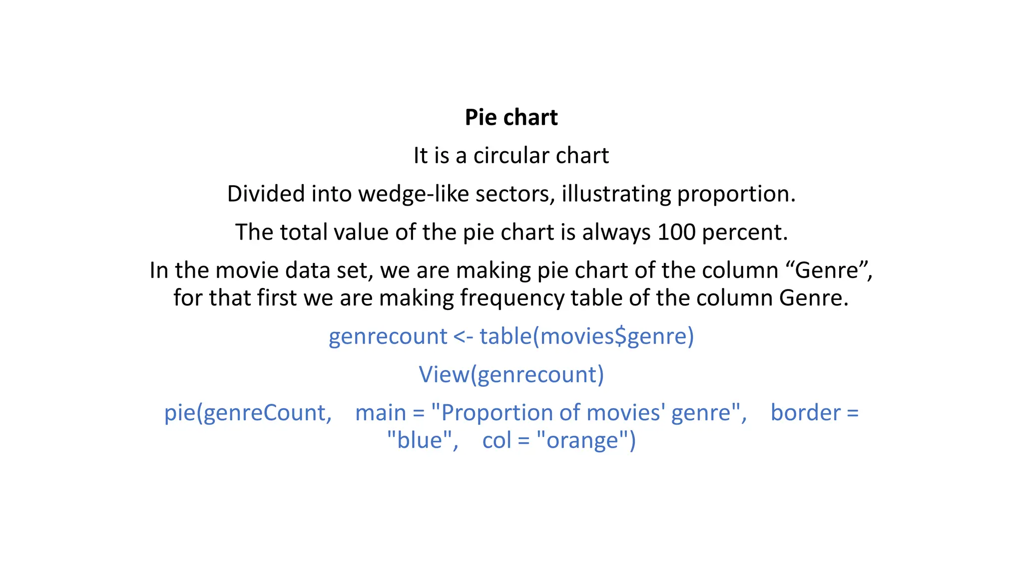
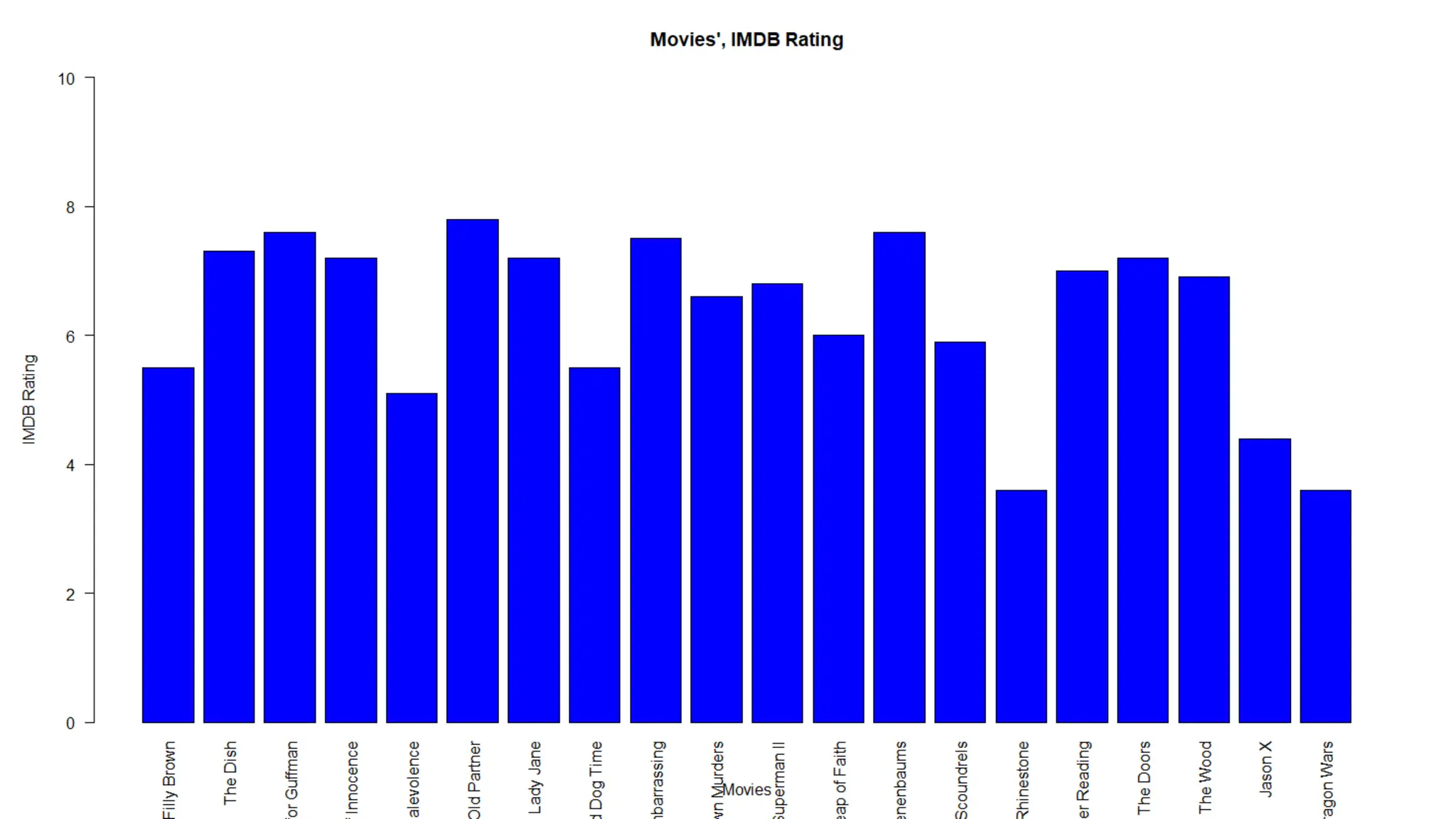
![Bar Chart A bar chart represents data in rectangular bars with length of the bar proportional to the value of the variable. R uses the function barplot to create bar charts We are plotting bar chart from the movie dataset, of the column imdb_ratings and for the sake of simplicity we are taking only 20 observations. moviesSub <- movies[1:20,] barplot(moviesSub$imdb_rating, ylab = "IMDB Rating", xlab = "Movies", col = "blue", ylim = c(0,10), main = "Movies', IMDB Rating")](https://image.slidesharecdn.com/basicsofrprogrammingforanalyticsautosaved1-240916080545-0682f8c8/75/Basics-of-R-programming-for-analytics-Autosaved-1-pdf-32-2048.jpg)


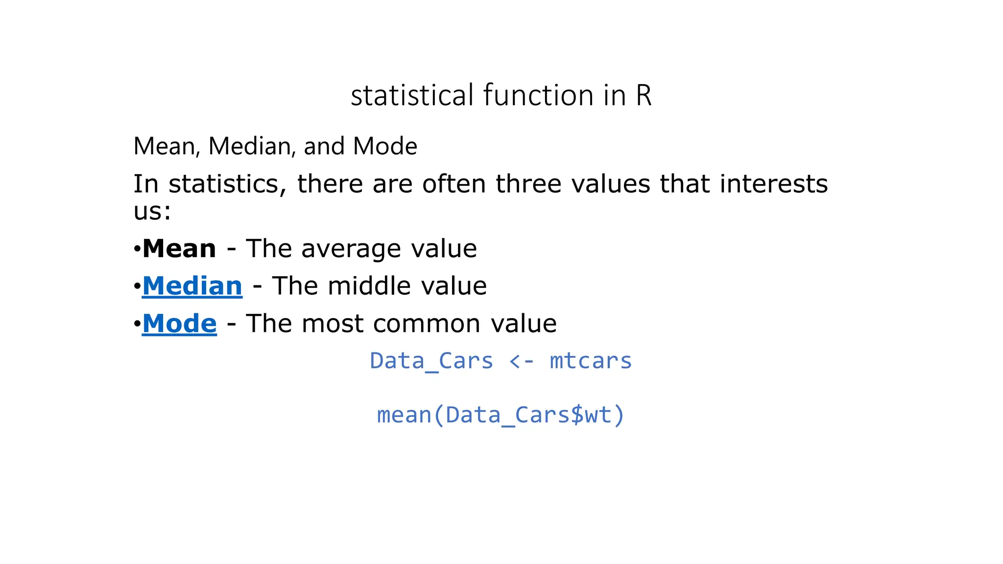
![Mode The mode value is the value that appears the most number of times. R does not have a function to calculate the mode. However, we can create our own function to find it. If we take a look at the values of the wt variable (from the mtcars data set), we will see that the numbers 3.440 are often shown: Data_Cars <- mtcars names(sort(-table(Data_Cars$wt)))[1]](https://image.slidesharecdn.com/basicsofrprogrammingforanalyticsautosaved1-240916080545-0682f8c8/75/Basics-of-R-programming-for-analytics-Autosaved-1-pdf-75-2048.jpg)