Downloaded 183 times

![Encoder Vector Representation We define n binary vector with K elements (one vector for each modulo-2 adder) The i-th element in each vector, is “1” if the i-th stage in the shift register is connected to the corresponding modulo-2 adder, and “0” otherwise. Examples: k=1 1 1 1 1 0 1 𝑔1 = 1 1 1 𝑔2 = [1 0 1] 𝑔1 = 1 0 0 𝑔2 = 1 0 1 𝑔3 = [1 1 1] Generator matrix with 2 vectors Generator matrix with 3 vectors](https://image.slidesharecdn.com/presentationconvolutionerrorcontrolcoding-160701041407/75/Convolutional-Error-Control-Coding-12-2048.jpg)


![MATLAB Simulation: BER, Time Performance Convolutional-Viterbi Codec Generator Vector : [111,101] Hard and Soft Decisions Block Codec Hamming (7,4) Hard and Soft Decisions Vs. Richard Hamming Andrew J. Viterbi](https://image.slidesharecdn.com/presentationconvolutionerrorcontrolcoding-160701041407/75/Convolutional-Error-Control-Coding-32-2048.jpg)


The document discusses convolutional error control coding, detailing its structure, representations, and the Viterbi algorithm for optimum decoding. It compares various error control techniques, including Automatic Repeat Request (ARQ) and Forward Error Correction (FEC), and illustrates the effectiveness of convolutional codes over block codes. Additionally, it includes MATLAB simulation analyses for bit error rates and decision-making trade-offs.
Introduction to MEH607 Error Control Coding course offered at Kocaeli University by Mohammed Abuihaid.
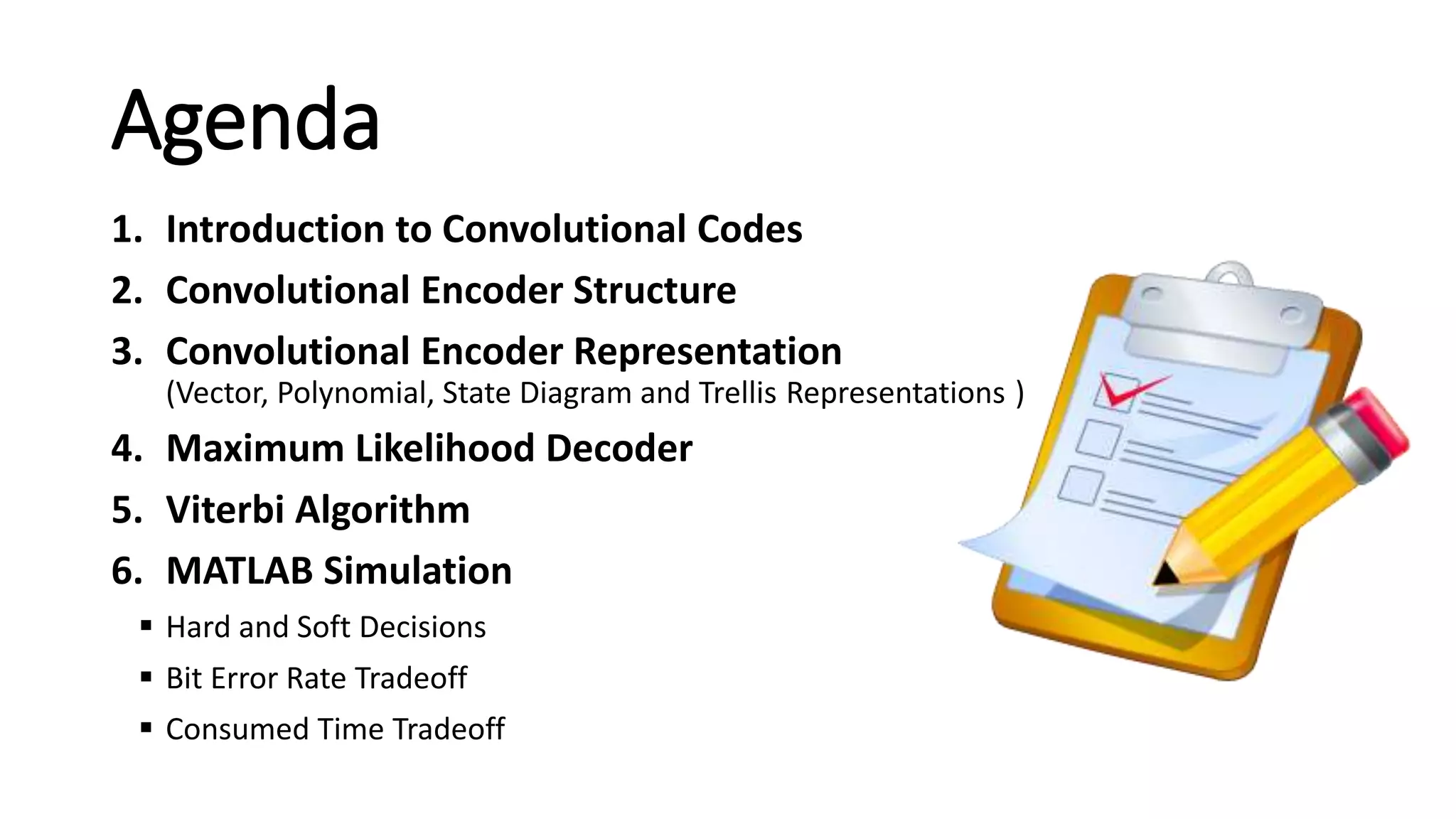
Outline of presentation topics including convolutional codes, encoder structures, decoding algorithms, and MATLAB simulation.
Explains ARQ, FEC, and Hybrid ARQ techniques, emphasizing reliability, data rates, and application to wire-line and wireless communications.
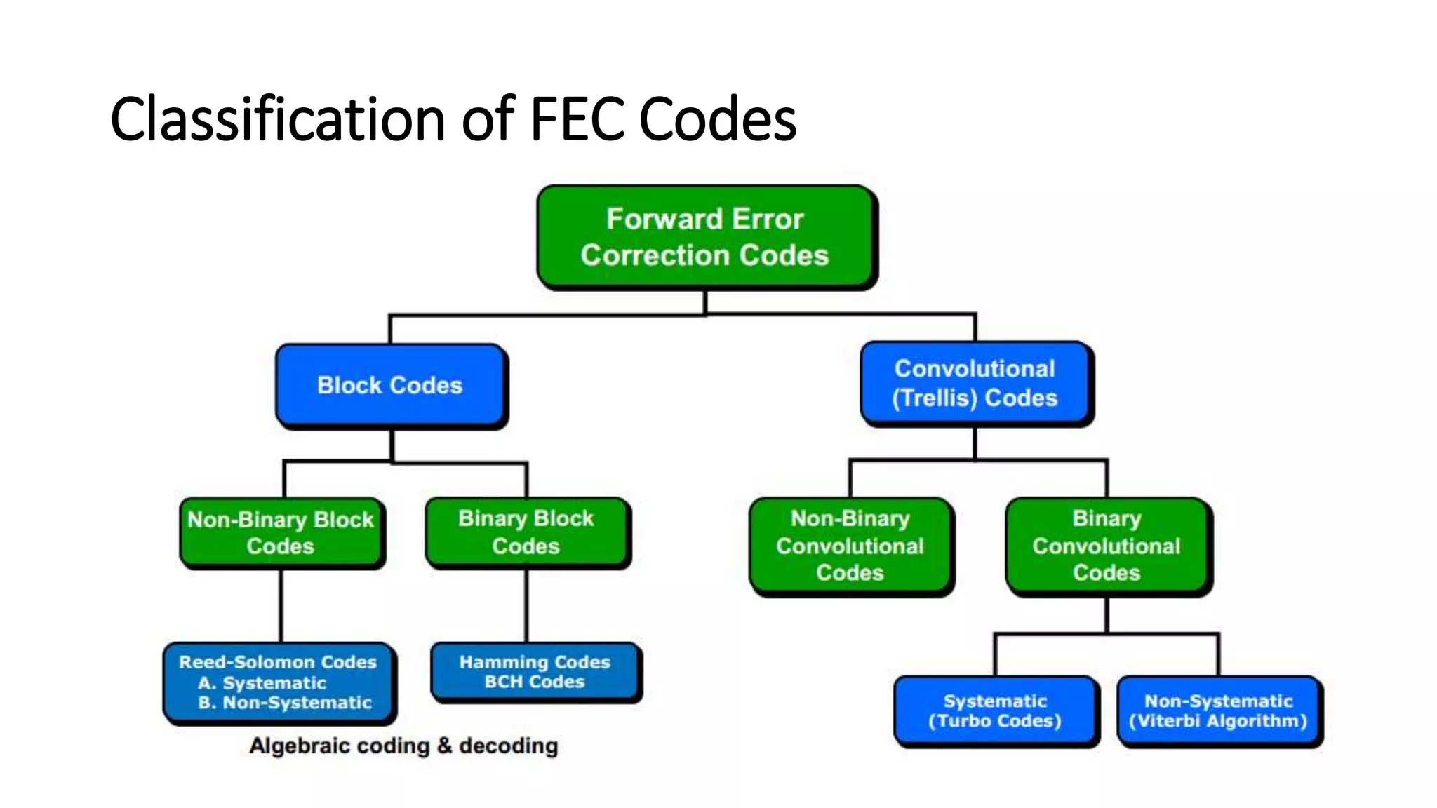
Discussion on classification of Forward Error Correction (FEC) codes.
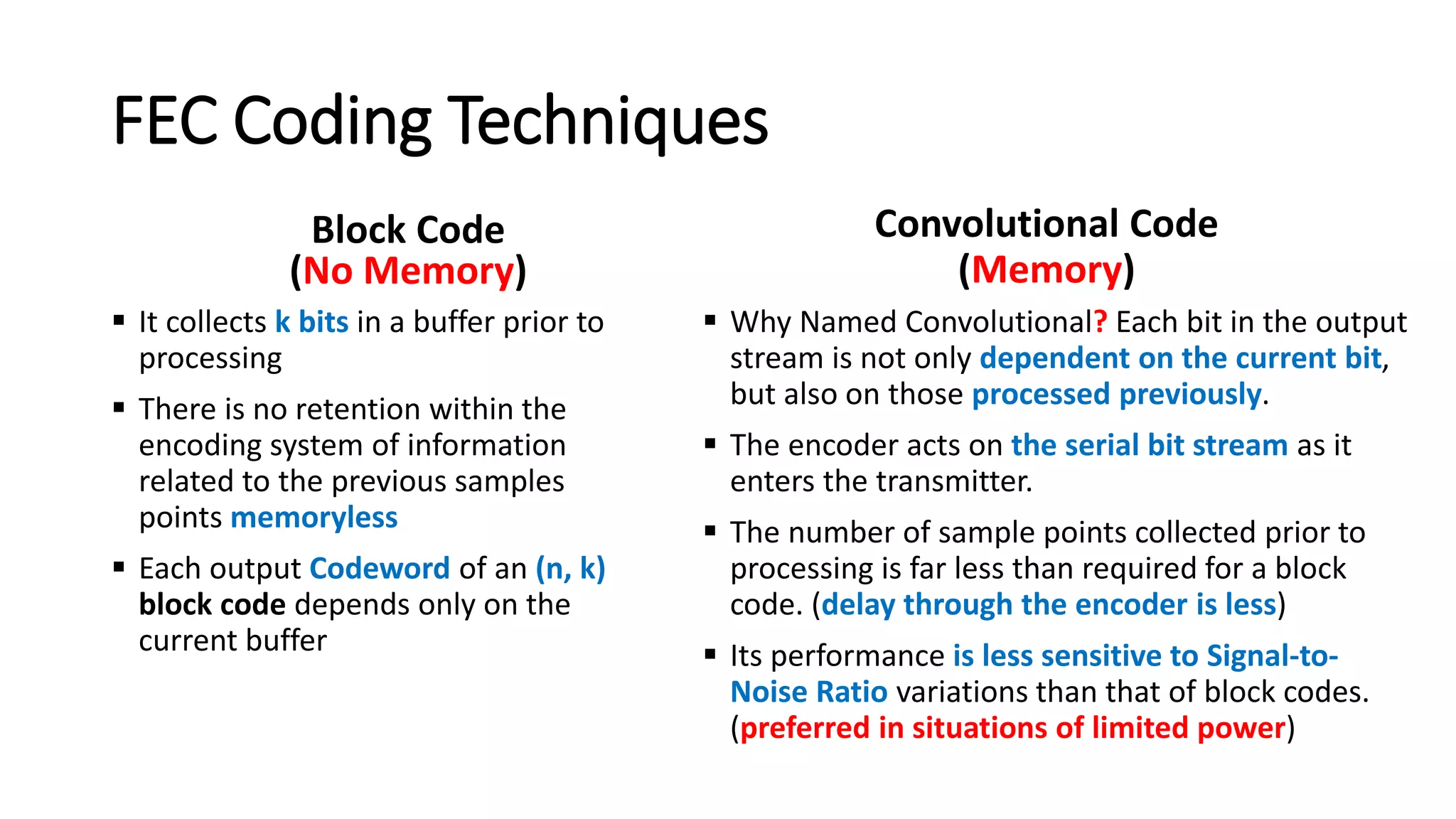
Comparison of Block and Convolutional Codes, highlighting memory aspects and performance in error sensitivity.
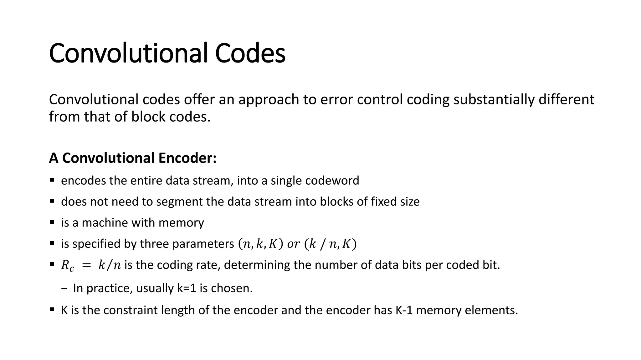
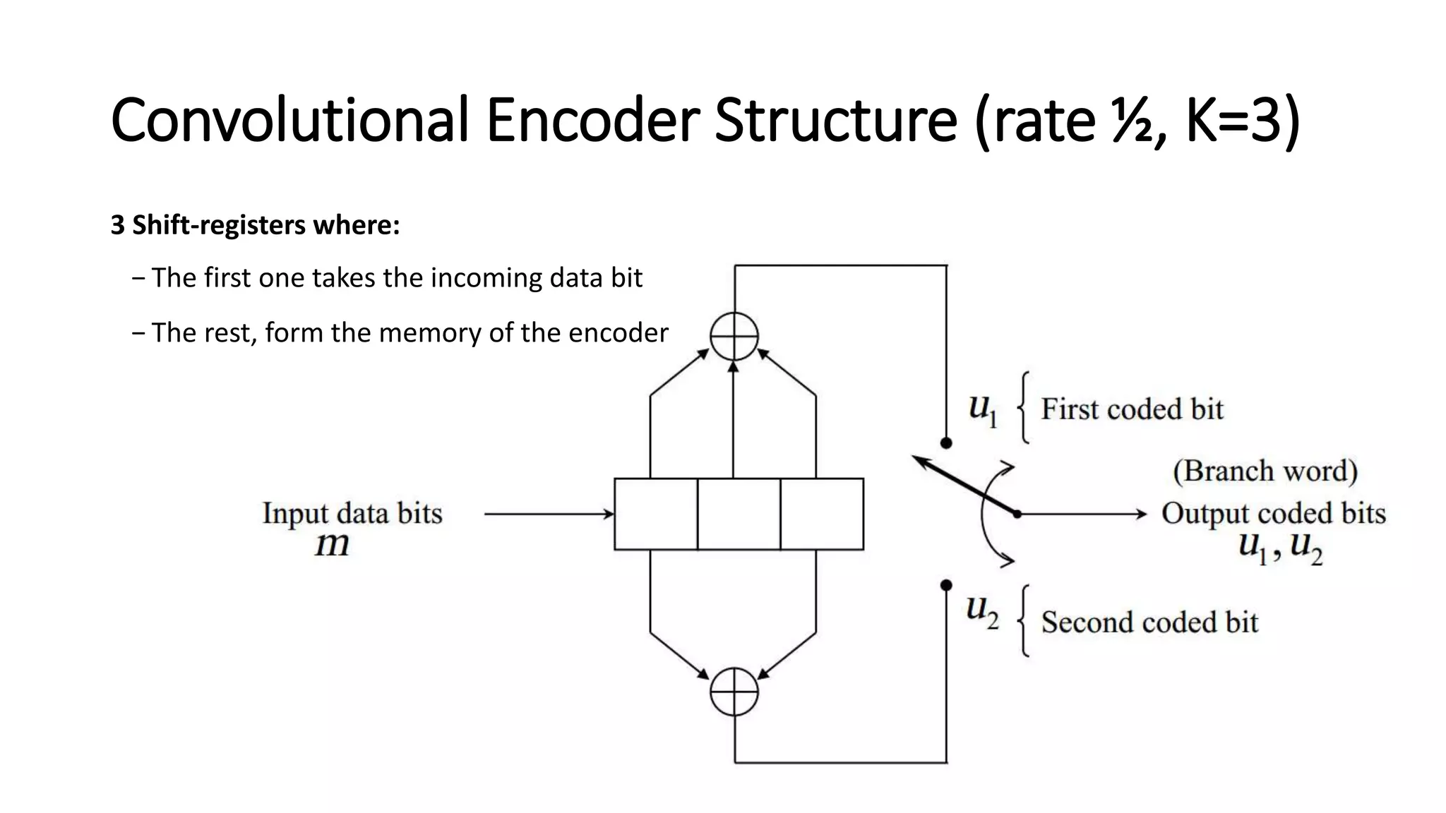
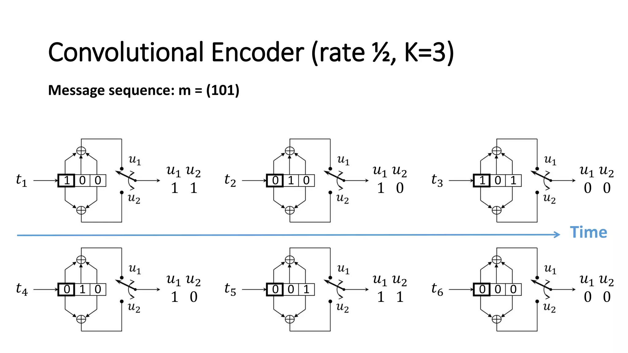
Details on convolutional codes, advantages over block codes, and definitions of coding rate and constraint length.
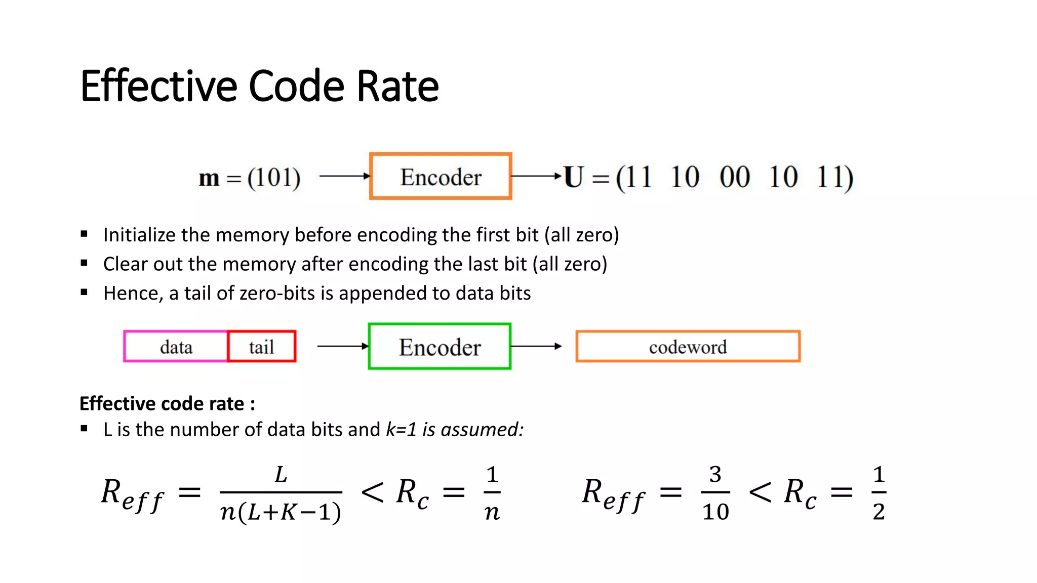
Details on the structure of a convolutional encoder with specific parameters, effective code rates, and tail-bit addition.
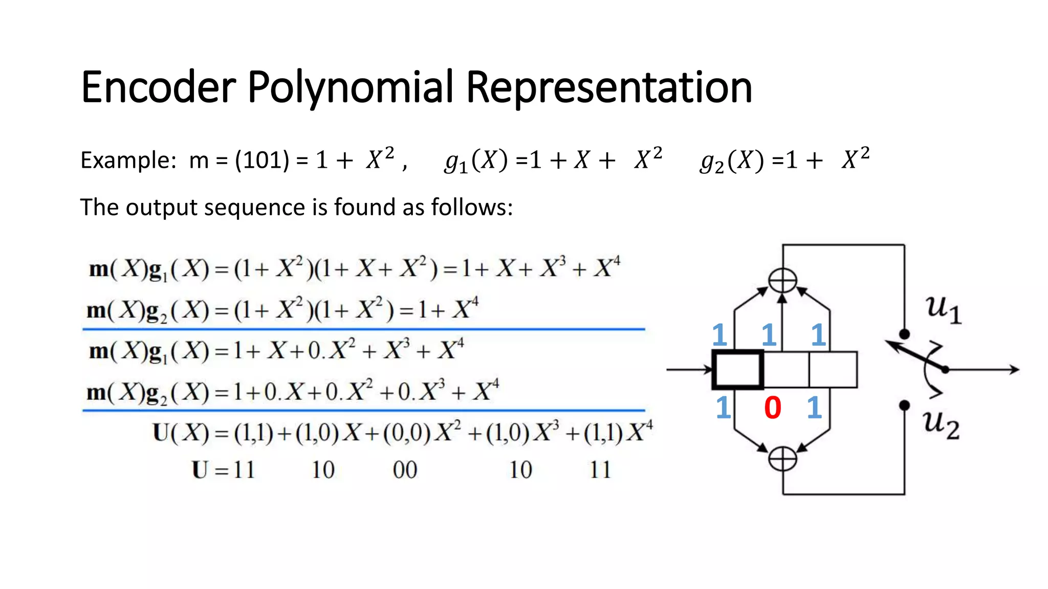
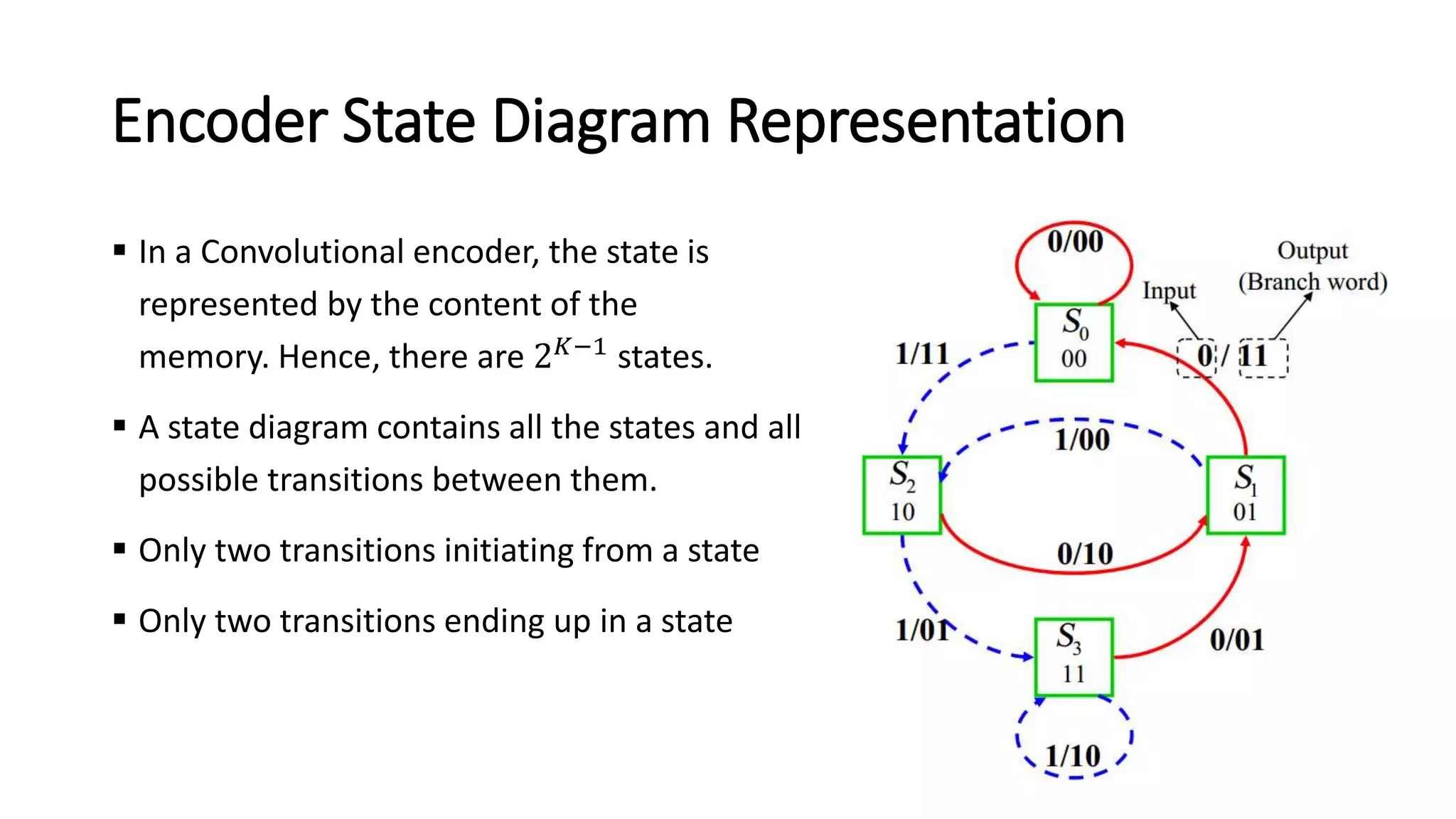
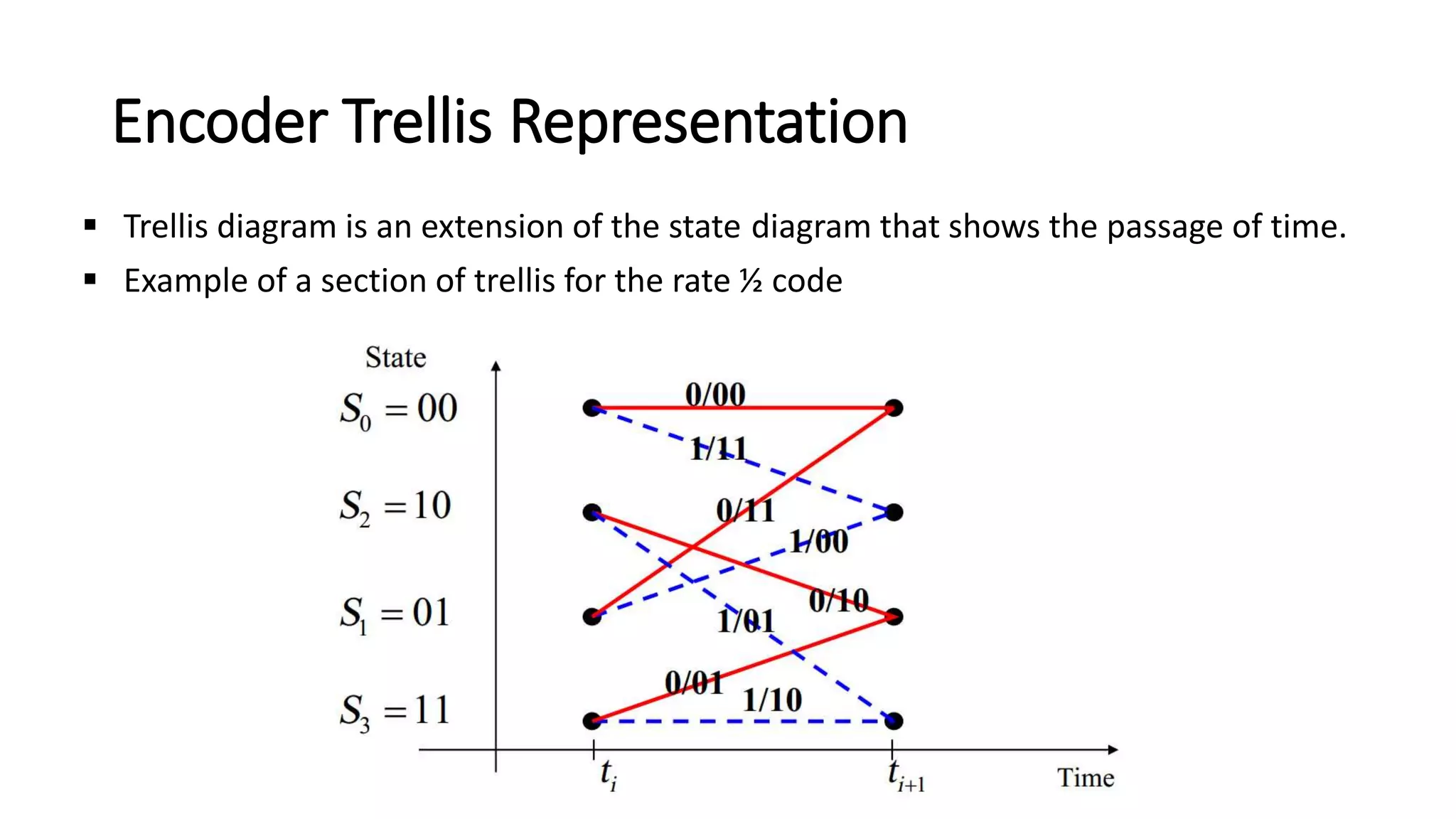
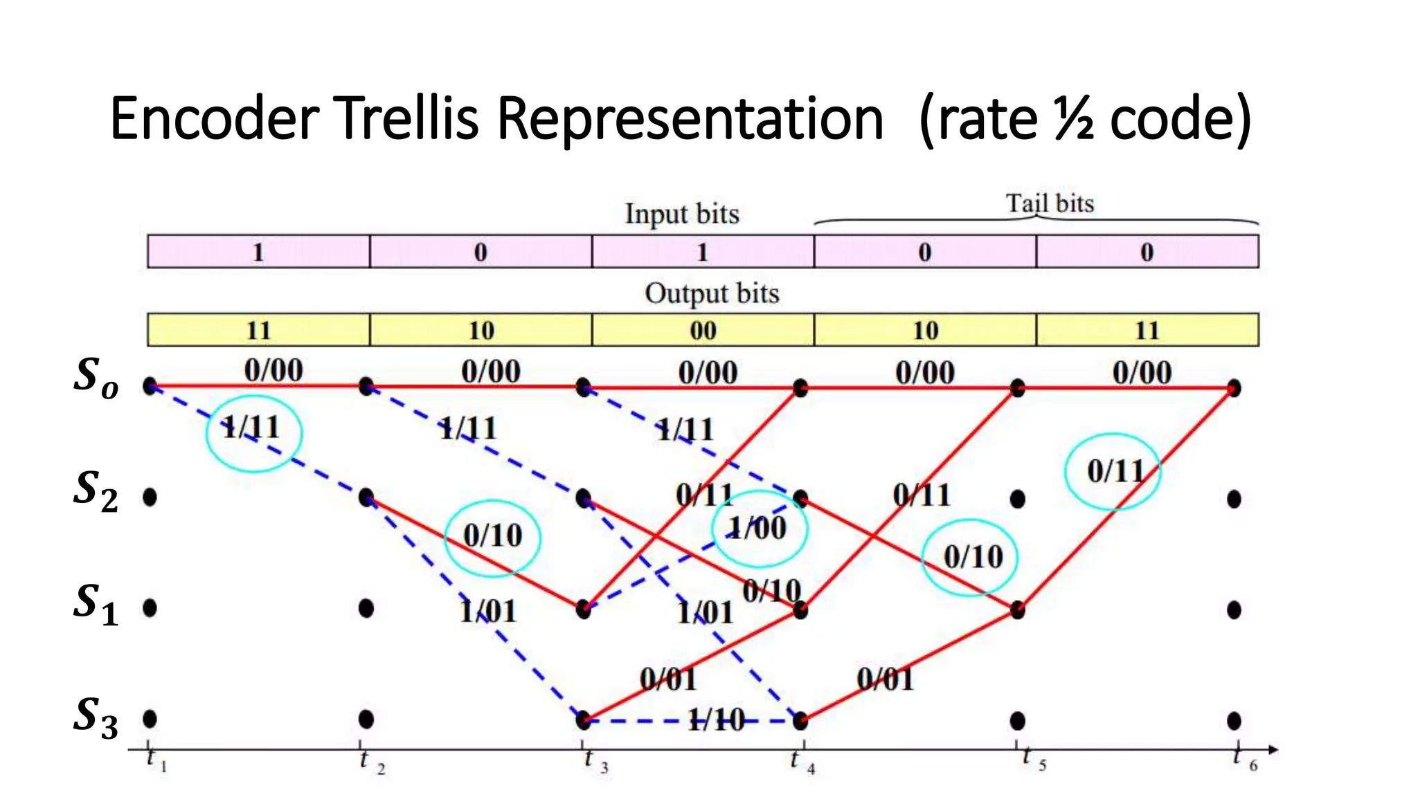
Explanation of vector, polynomial, state diagram, and trellis representations of convolutional encoders.
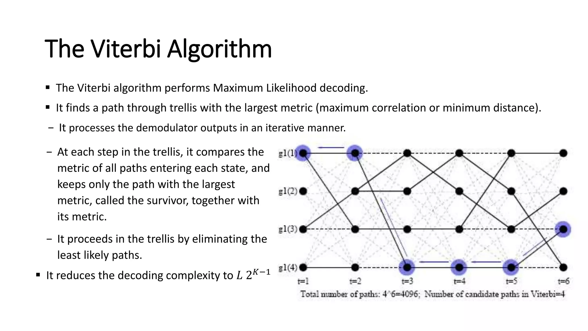
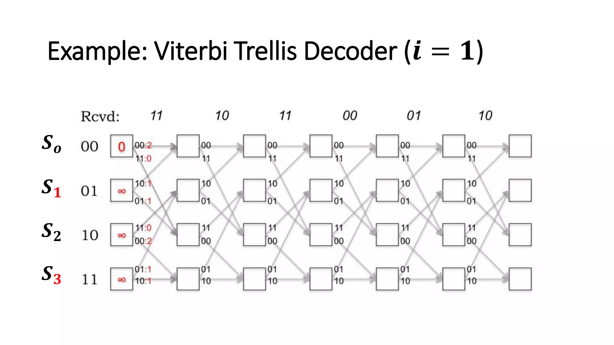
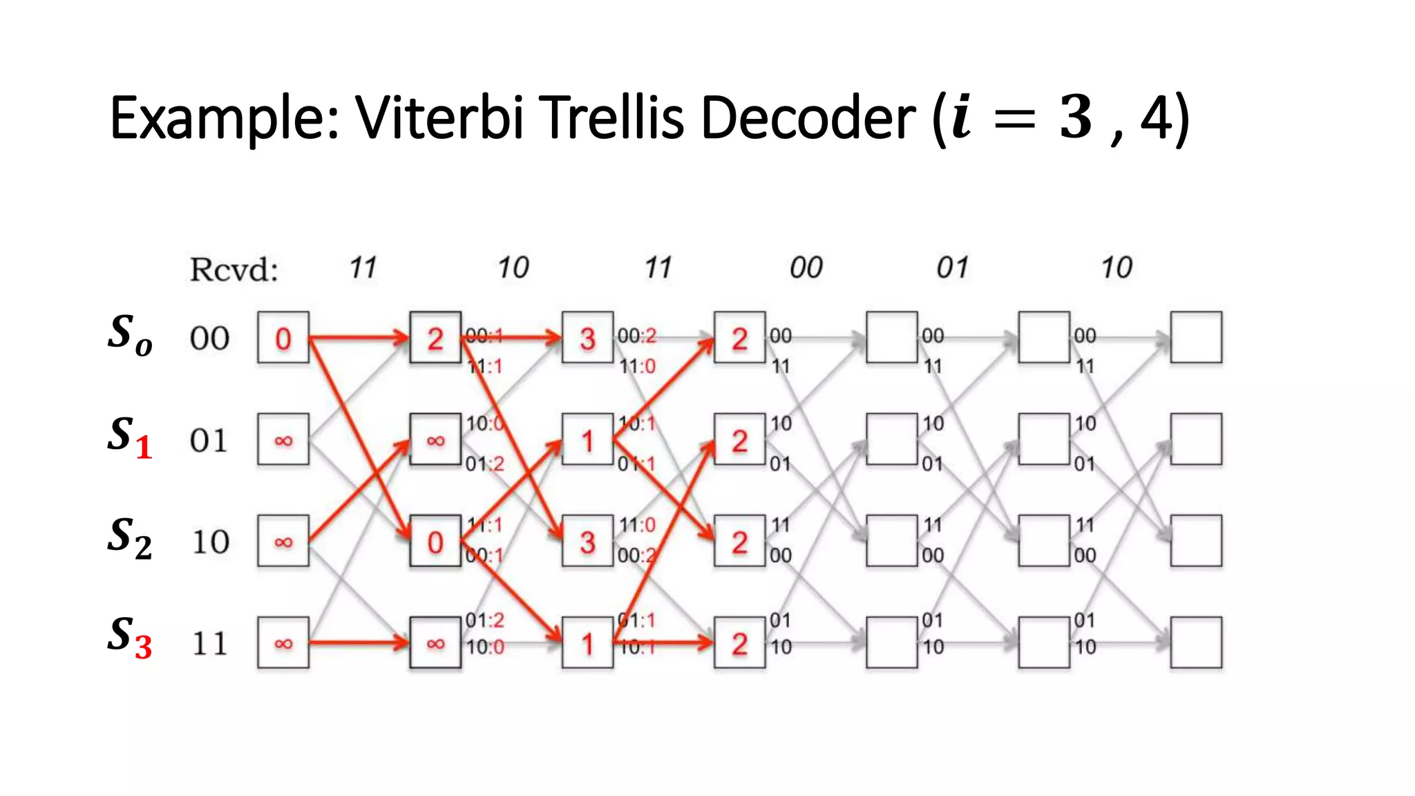
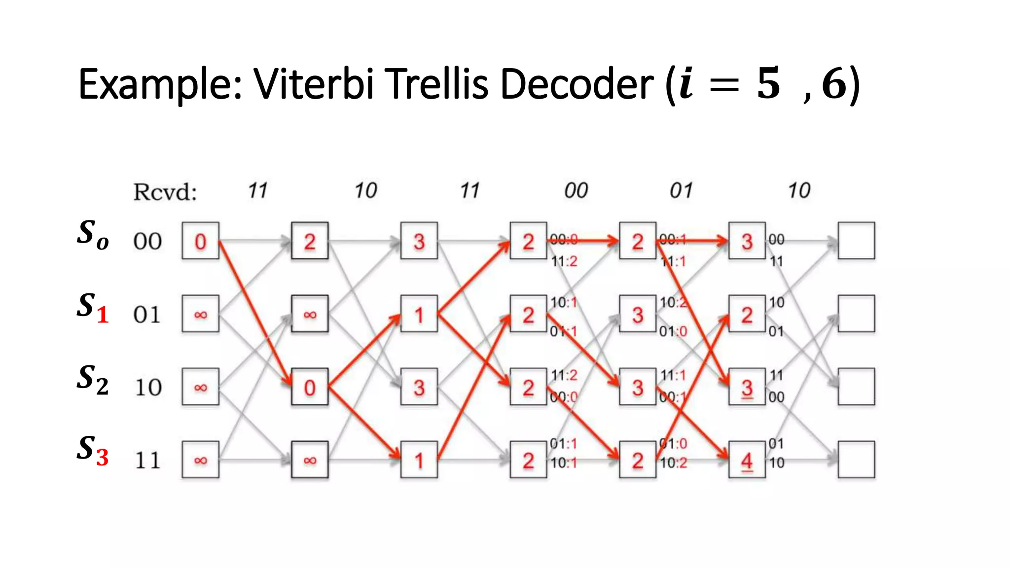
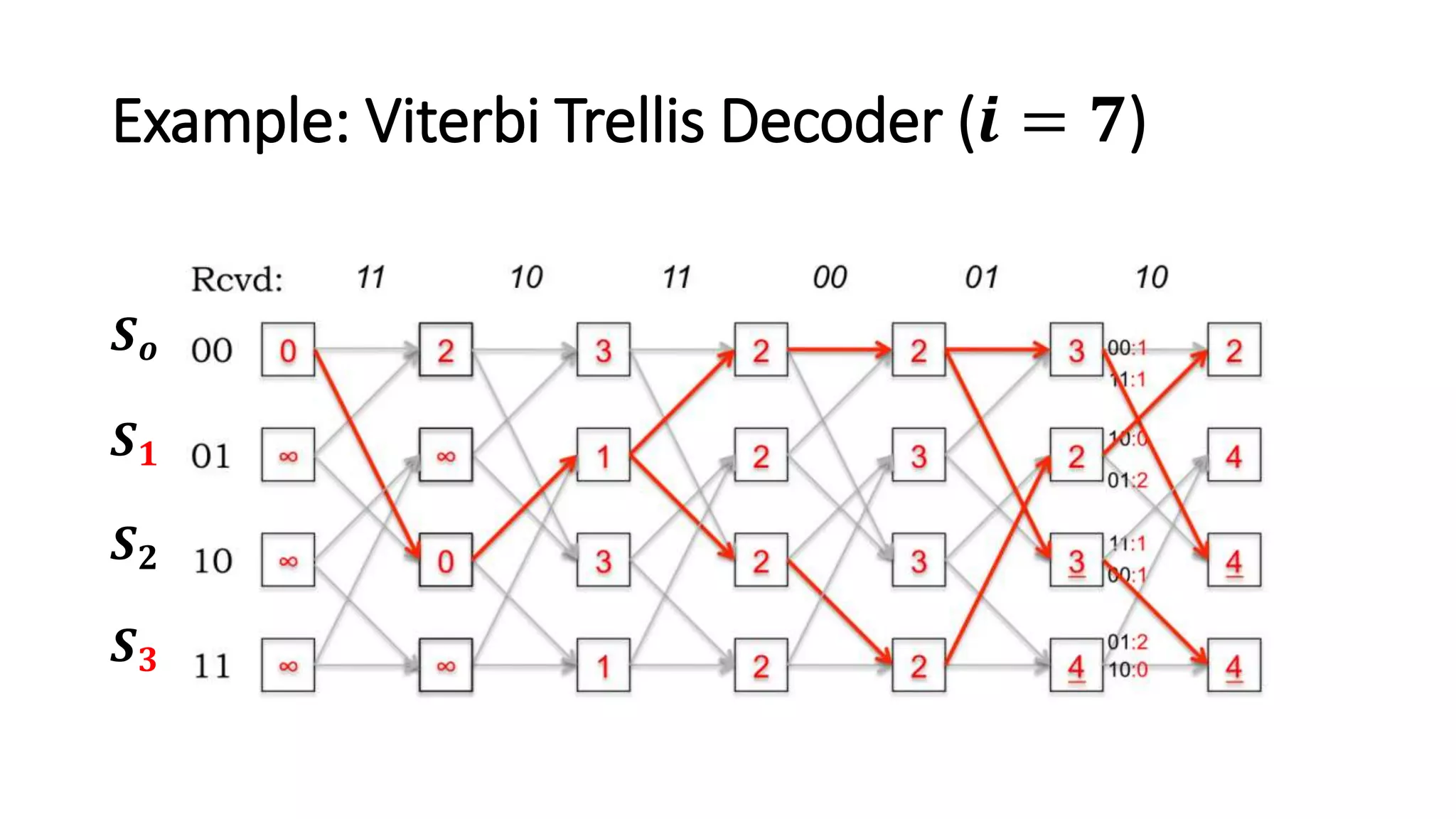
Describes the Maximum Likelihood decoding method and the Viterbi algorithm used for path finding in trellis diagrams.
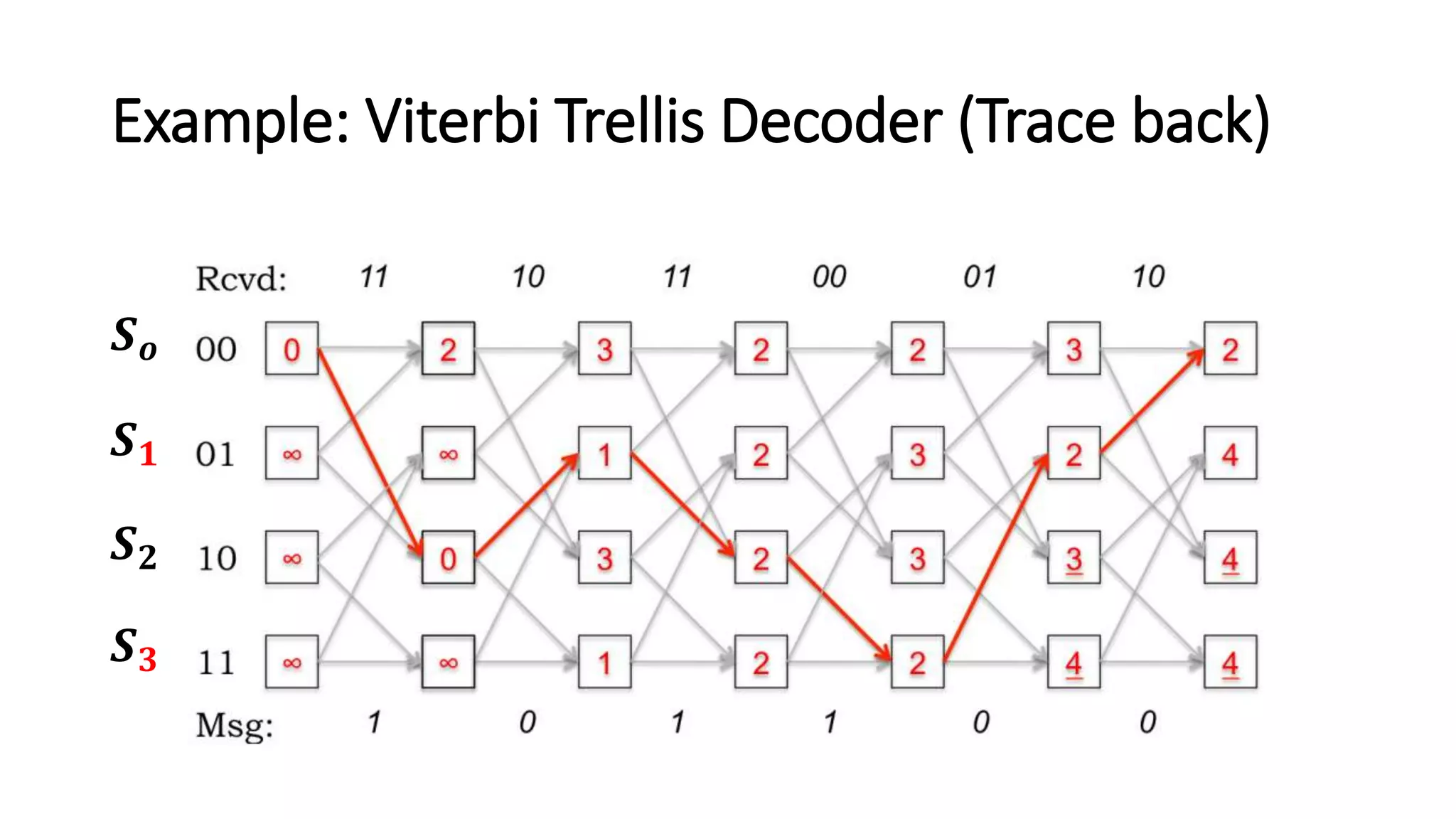
Example of a convolutional trellis encoder and the step-by-step Viterbi decoding process through the trellis.
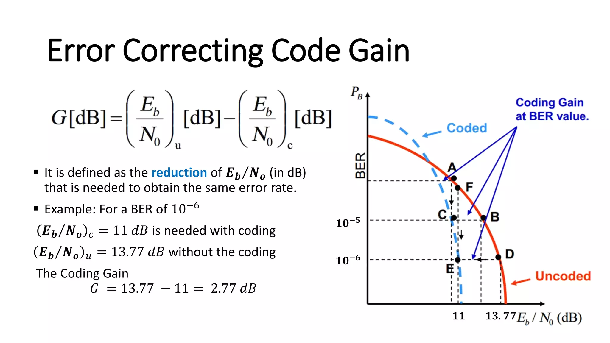
Defines coding gain, showing the importance of reducing energy per bit to noise ratio for improved error rates.
Details about MATLAB simulation related to bit error rates and performance comparisons between different codecs.
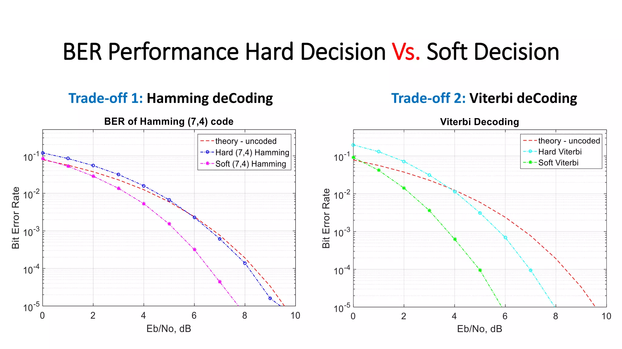
Discusses the trade-offs in error performance between Hard vs. Soft decisions in various coding schemes.
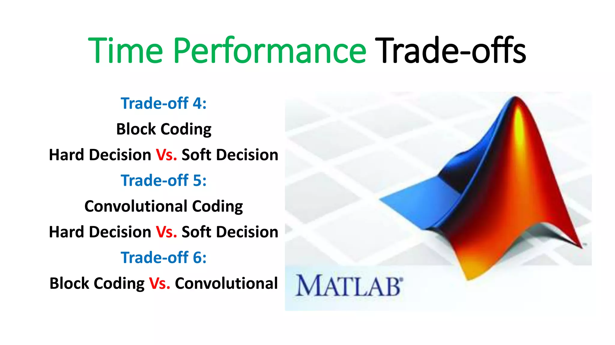
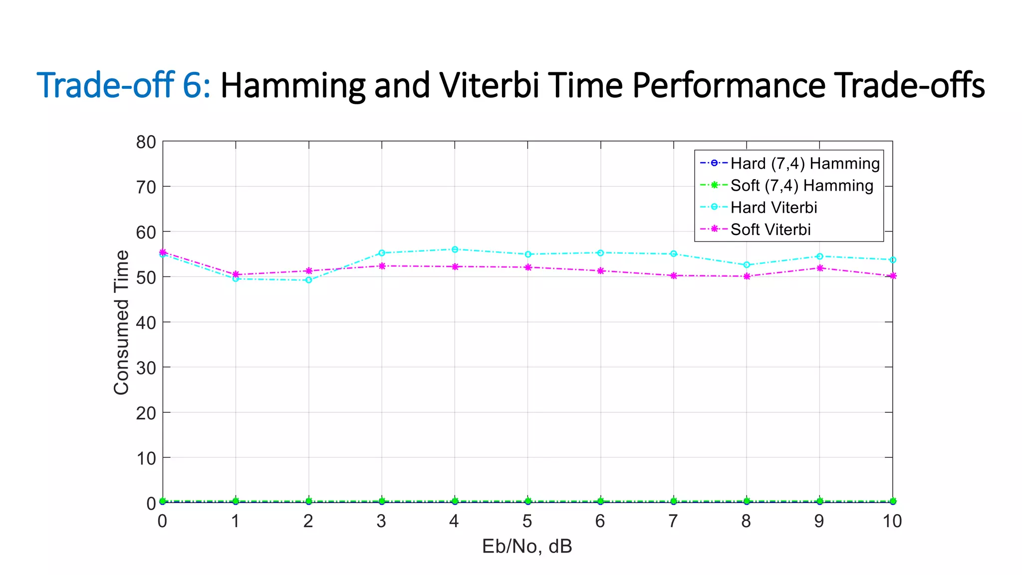
Covers trade-offs in time performance across different coding techniques and their impacts on efficiency.
Presentation conclusion with personal sign off by Mohammed Abuibaid, emphasizing engagement with wireless technology.