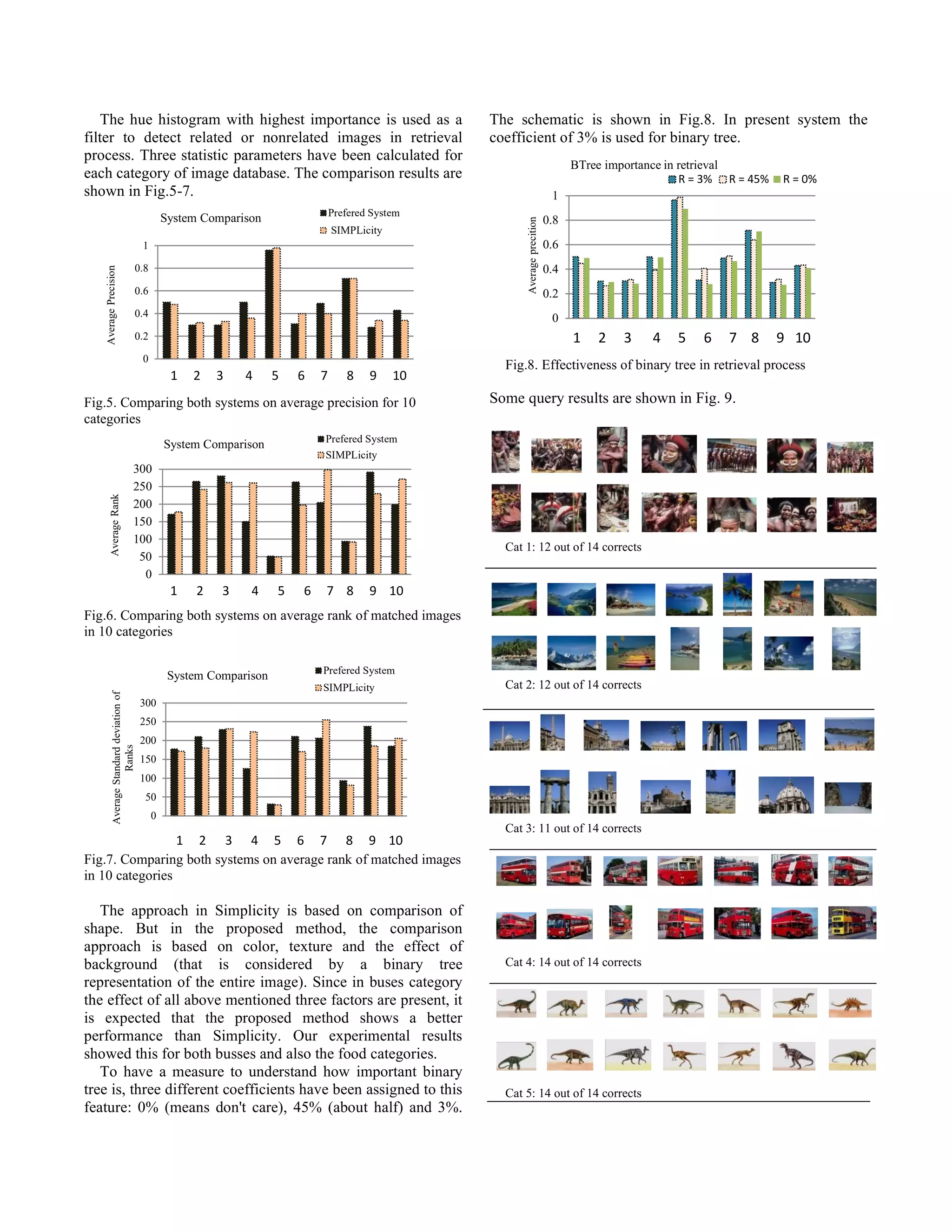
Content-based Image Retrieval Using The knowledge of Color, Texture in Binary Tree Structure

Content-based Image Retrieval Using The knowledge of Color, Texture in Binary Tree Structure

• 1.
  Content based imageretrieval using the knowledge of texture, color in binary tree structure Zahra Mansoori, Mansour Jamzad Z_mansoori@ce.sharif.edu, Jamzad@sharif.edu Sharif University of technology, Tehran, Iran ABSTRACT Content base image retrieval is an important research field with many applications. This paper presents a new approach for finding similar images to a given query in a general- purpose image database using content-based image retrieval. Color and Texture are used as basic features to describe images. In addition, a binary tree structure is used to describe higher level features of an image. It has been used to keep information about separate segments of the images. The performance of the proposed system has been compared with the SIMPLIcity system using COREL image database. our experimental results showed that among 10 image categories available in COREL database, our system had a better performance (10% average) in four categories, equal performance in two and lower performance (7% average) for the remaining four categories. Index Terms— Content-based Image retrieval, Color, texture, Binary Tree Partitioning 1. INTRODUCTION In recent years, content-based image retrieval (CBIR) has played an important role in many fields, such as medicine, geography, weather forecasting, security, etc. These approaches are based on visual attributes of images such as color, texture, shape, layout and object. Most of the content-based image retrieval systems are designed to find the top N images that are most similar to the user query image [1, 2]. In this paper the approach is to combine color, Texture and a customized binary partitioning tree in order to find the images similar to a specific query image. The above mentioned tree is a customized binary partitioning tree which keeps a combination of color and layout information of an image. To extract color information, two histograms of the image in HSV mode are used with 360 and 100 bins. Also a 2-levels Wavelet decomposition of separated image blocks is used to attain texture. The binary tree is used to maintain information about separated regions of the image. 2. OVERALL STRUCTURE The overall structure of almost all CBIR systems typically consist of two Independent parts: Feature Extraction and Retrieval. The first part extracts visual information from the image and saves them in a database, where the second part searches the maintained information based on defined conditions to find the matching images from database. The details of composition and functionality of these parts vary among different systems. The overall structure of a typical image retrieval system is shown in Fig.1, which has seven separated parts: 1. Image database consisting of hundreds or thousands of images among which a query image is searched; 2. Feature Extraction which retrieves features from images and sends them to appropriate parts; 3. Database of extracted features received from part 2; 4. Query image which is an image input by the user in order to get the similar images; 5. Feature Vectors of query image extracted by part 2; 6. Search and retrieval part which searches the Feature Vectors database in order to get similar images to query image; 7. User interface which shows the retrieved images from part 6. Fig.1. Overall structure of an image retrieval system (from ] 3 , 4 [ ) In the proposed approach, feature extraction is divided into two levels, low level feature extraction that extracts Color and Texture features, and the description of Binary Tree Structure in retrieval process. 3. FEATURE EXTRACTION Technically, any image can be considered as a 2- Dimonsional array of pixels. Feature extraction is a way to show visual information of an image in scale of numbers so they can be analogous. 4. Query Image 5. Query Image F.V. 1. Image DB 3. F.V.s DB 6. Search and Retrieval 7. End user 2. Feature Extraction
• 2.
  3.1. Color Extraction Coloris represented in a 3-channel color space. There are various color spaces such as RGB, HSV, YCbCr, CIE LAB, CIE LUV, etc. however, no color space is dominant in all applications. In this paper, the HSV color space is used because it is a perceptual color space. That is, the three components H (Hue), S (Saturation) and V (Value) correspond to the color attributes closely associated with the way that the human eye perceives the color. Hue indicates the type of color, such as red, green and blue, which corresponds to the dominant wavelength of a given perceived color stimulus. Saturation refers to the strength of a color. A fully saturated color contains only a single wavelength. The color becomes less saturated when white light is added to it. Value (or intensity) is the amount of light perceived from a given color sensation. White is perceived to be maximum intensity and black to be the minimum intensity The approach here is two extract two histograms, one for Hue and one for Saturation. Due to the fact that the Value dimension of color in HSV is too variant by lightness degree of photography, so it is not a valid measure to judge how two images are similar, so it is not considered in calculation. The Hue circle of HSV color space has been quantized into 360 degrees, and saturation into 100 levels. Thus the corresponding histograms have 360 and 100 bins. 3.2. Texture Extraction Texture is a key component of human visual perception. Like color, texture is an essential feature to be considered when querying image databases [5]. Generally speaking, textures are complex visual patterns composed of entities, or sub-patterns which have characteristic brightness, color, slope, size, etc. Therefore texture can be regarded as a similarity grouping in an image [6]. For texture extraction, Wavelet decomposition of image blocks is used. By imposing Wavelet on a gray-level image, four sub images will be produced, which is a low resolution copy (Approximation) image, and three-band passed filters in specific directions: horizontal, vertical and diagonal respectively. These sub images contain useful information about image texture characteristics. To have a numerical presentation of the texture, mean and variation of these images will be calculated. Final feature vector will be gained by 1. Dividing image into 8×8 = 64 equal blocks; 2. Applying Wavelet on each block. 3. Calculating Mean and Variation of each block and concatenating them, separately; 4. Concatenating all obtained feature vectors to achieve two feature vectors describing texture information. 3.3. Binary Partitioning Tree A Binary Partition Tree is a structured representation of the regions of an image. An example is shown in Fig.2. The leaves of the tree represent regions belonging to the initial partition (partition 1) and the remaining nodes represent regions that are obtained by merging the regions represented by the two children of a node. The root node represents the entire image. This representation should be considered as a compromise between representation accuracy and processing efficiency. The main advantage of the tree representation is that it allows the fast implementation of sophisticated partitioning process [8]. Fig.2. An example of Binary Partition Tree creation with a region merging algorithm (derived from [8]) In this paper, a simplified and efficient use of binary tree has been proposed. There are some important considerations in the way to create the partitioning tree to obtain better performance. 3.3.1. Image Partitioning There are various ways to partition an image into separate regions, but the most important consideration is that each partition should be meaningful, which in best case, contains dedicated information about an object. An object may have a homogeneous color [8], Color & texture [9] or none which in this case, defining an object may be impossible and this case can be eliminated. The approach of this paper is based on color homogeneity; batches of similar colors will signify objects/regions. This is achieved by using safe color cube as a primary color palette. It is demonstrated that this palette works well as it covers RGB color space as well, which after quantization, well equivalent of row image will be gained. Safe Color Cube consists of 216 colors in RGB mode; each R, G and B can only be 0, 51, 102, 153, 204 or 255. Thus, RGB triples of these values give us (6)3 = 216 possible values [10] (Fig. 3.). To represent a picture, for each pixel or batch of pixels the equivalent color in the palette will be found and replaced. For better precision, mean of a batch of pixels should be used. New color will be replaced with the old one. This process is called quantization. By having an image with 216 specific colors, it is expected to have distinctive regions with homogeneous color. By converting this image to gray-scale, we have a partitioned image. The number of possible gray-levels will be 216.
• 3.
  3.3.2. Tree Construction Toconstruct a binary tree, the algorithm starts from an arbitrary region as the first node and chooses a neighbor region as its sibling and these nodes will be added as children of their parent node. This process will be repeated until all regions have been added to the tree. To construct the binary tree an important point is that the trees must be comparable with each other. One way to achieve this is to define a fixed template for trees such that the comparison will be done node by node. The constrains of constructing the trees is to define 1. Maximum levels of the tree and 2. Maximum regions that the image will be partitioned at each level of partitioning. Doing this, all images are represented by identical trees with equal number of levels and nodes. The remaining problem is whether two similar images will produce the same trees? How different the trees will be if their corresponding images had little differences. It is possible that in each level, the region in two similar pictures are segmented differently, so the starting points at each level will be different and the resulting trees may be completely or partially incomparable. The technical solution for the problem of similar images is to define fixed regions at the starting point, away from previously mentioned partitioning. If the size of these fixed-sized regions is large, the problem still remains; if they are small, the presence of the tree is meaningless. The trade off may be to initialize constructing by fixed size regions like what we used for texture extraction approach. The approach here is to divide the image into equal-sized regions and creating a distinct tree for each region. Fig.3 shows an iterative algorithm for tree construction, inputs are 1. Colored image and 2. Number of maximum growing levels of tree, and the output is a tree, representing the image. INITIALIZE (MaximumTreeLevels, MaximumRegions) GrayImage = LebeledBySafeColors ( Image) MaxTreeL = MaximumTreeLevelsDefines MaxReg = MaximumRegions BINARYTREE_ITERATIVE_CONST(GrayImage, 0) BINARYTREE_ITERATIVE_CONST(GrayImage, CurrentTreeL ) If CurrentTreeL = MaxTreeL Return Save( BINARY TREE_GETPROPERTIES ( GrayImage ) ) GMin = MinimumGrayLevelsOf ( GrayImage ) GMax = MaximumGrayLevelsOf ( GrayImage ) GStepsizes = ( MaxG – MinG ) / MaxReg For i = 1 to MaxReg LowestG = ( i – 1 ) * GStepsizes + GMin HighestG = i * GStepsizes + GMin SubImage=FilterGrayLevels ( GrayImage, LowestG, HighestG ) BINARYTREE_ITERATIVE_CONST(SubImage,CurrentTreeL+1) End Fig.3. Pseudo code algorithm for binary tree construction 3.3.3. Features Final feature extraction will be the mean color and the surface of the regions at each node (internal or leaves). Surface is the number of pixels in a region, if all images are normalized then it means we have equal sizes. Due to usage of SIMPLicity database for comparison, all images have approximately the same size so it is safely assumed that the whole database is normalized. 4. SEARCH AND RETRIEVAL After extracting features, the second main responsibility of an image retrieval system is 'Search and retrieval'. It is assumed that feature space is a multidimensional space and images are scattered based on the value of their feature vectors, so more similar the feature vector, closer are images in this space. The Search process is to get feature vectors of an input image called 'Query' or 'Feed' [11] and retrieve the images in the neighborhood of that in feature space. This search strategy is called nearest-neighborhood [12]. If we assume that two images of database are more similar than the others, their feature vector should have a minimum distance; so the similarity has a reversed relationship with the distance. So by having the difference of feature vectors of two images, the similarity of them will be known. 4.1. Distance measure The difference of two feature vectors should be defined in a way that it appears perfectly as it has close relationship to the type of feature. Most of the difference formulas are a variation of Minkowski difference. The Minkowski distance for two vectors or histograms ~k and ~l with dimension n is given by equation (7) [3]. 𝐷 𝑘, 𝑙̅ = ( |𝑘 − 𝑙 | ) / (7) Color histogram is usually measured by 𝜌 = 1 [13, 14], so this measure is used in our approach too. For texture level, two of the remaining distances have been used. This form is called Euclidean distance. Binary tree is a special case due to the type of its features. There is a Matrix of 3-dimentional colors and an array of surfaces. For color distance, the distance between colors of each node is calculated by using Euclidean distance and finally the results have been aggregated. For the surface the same distance metric as histogram has been used. There may be a case that a specific region assigned to an internal node has a unique gray level such that it could not be divided into some sub-regions and one of its children in binary tree may have zero value for Color and Surface property. At the time of calculating the difference, these nodes will not be accounted and the judgment is based on its higher levels or its sibling.
• 4.
  4.2. Final QueryRanking Finally, the feature distances should be summed in order to have a final distance. The prerequisite for this operation is normalization in each feature level, by dividing all distance values of a specific feature to the maximum gained distance. Adding all the difference values gets a measure of how an image is different from the query image. By reversing this value, the 'Rank' of each image will be calculated. The most k high-rank images will be chosen to display to the user. The main issue for each feature at the retrieval level is how efficient it is; in other words how much of the performance of the system depends on it. To make it clear there are coefficients assigned to each feature vector. Final ranking will be achieved from equations (8) ~ (11). 𝑟 = 𝑟 , + 𝑟 , + 𝑟 , (8) 𝑟 , = 𝑅 . 𝑆 , (9) 𝑆 , = 1/𝐷𝑠 , (10) 𝐷𝑠 , = 𝐷 , 𝑀𝐴𝑋 𝐷 , (11) Where in 8, ri is final rank of ith image, 𝑟 , , 𝑟 , , 𝑟 , are ranks of Color, Texture and Binary Tree features, respectively. For instance, 𝑟 , is extended in (9). 𝑅 is the coefficient of Color feature. 𝑆 , is the similarity measure between the ith image and query image in case of Color. As shown in (10), it is reversely dependent to distance; 𝐷𝑠 , means the distance of ith image from query image. In (11) normalization is carried on by dividing the row difference of both feature vectors to the maximum in their fields. 5. SYSTEMATIC EVALUATION This system has been compared to SIMPLicity [15] which is an image retrieval system which uses color, texture, shape, and location. This system was evaluated based on a subset of the COREL database, formed by 10 image categories (shown in Table 2), each containing 100 pictures. ID Category Name ID Category Name 1 Africa people & villages 6 Elephants 2 Beach 7 Flowers 3 Buildings 8 Horses 4 Buses 9 Mountains & glaciers 5 Dinosaurs 10 Food Table 2. COREL categories of images tested Within this database, it is known whether any two images belong to the same category. In particular, a retrieved image is considered a match if and only if it is in the same category as the query. This assumption is reasonable since the 10 categories were chosen so that each depicts a distinct semantic topic. Every image in the sub- database was tested as a query and the retrieval ranks of all the rest images were recorded. Three statistics were computed for each query: 1) the precision within the first 100 retrieved images, 2) the mean rank of all the matched images, and 3) the standard deviation of the ranks of matched images. The recall within the first 100 retrieved images is identical to the precision in this special case. The total number of semantically related images for each query is fixed to be 100.The average performance for each image category is computed in terms of three statistics: p (precision), r (the mean rank of matched images), and σ (the standard deviation of the ranks of matched images). 6. EXPERIMENTAL RESULT The result of partitioning a sample image with 216-color palette is presented in Fig.4. After some experiments, the number of tree levels and number of regions is set to 4 and 2, respectively. By choosing these parameters, the number of empty regions has been reduced to minimum and each partitioned region will represent the image suitably. (a) (b) Fig.4. Binary Tree Construction: (a) original image (b) gray level of quantized image using 216-color palette In order to obtain the system performance, the first step is to define the importance of each feature. This has been done in a step by step procedure. At first, color has been tested with custom coefficients, in the second step a test on both color and texture is done by assigning random coefficients to texture. In the next step, the binary tree has been added to feature lists and proper coefficients have been assigned to it. The properties of each feature vector and their coefficients are listed in Table 3. i Visual Descriptor Feature Vector Importance (Ri) 1 Color 360-bin Hue Hist 68% 2 100-bin Sat Hist 14% 3 Texture Wavelet Mean 6% 4 Wavelet Var 6% 5 Binary Partitioning Tree Color Mean 3% 6 Surface 3% Table 3. Information of the features used in this approach It should be noted that the extended formulas (8)~(11) are written using nominal feature vectors. In fact, there are more than three features, which are listed in Table 3.
• 5.
  The hue histogramwith highest importance is used as a filter to detect related or nonrelated images in retrieval process. Three statistic parameters have been calculated for each category of image database. The comparison results are shown in Fig.5-7. Fig.5. Comparing both systems on average precision for 10 categories Fig.6. Comparing both systems on average rank of matched images in 10 categories Fig.7. Comparing both systems on average rank of matched images in 10 categories The approach in Simplicity is based on comparison of shape. But in the proposed method, the comparison approach is based on color, texture and the effect of background (that is considered by a binary tree representation of the entire image). Since in buses category the effect of all above mentioned three factors are present, it is expected that the proposed method shows a better performance than Simplicity. Our experimental results showed this for both busses and also the food categories. To have a measure to understand how important binary tree is, three different coefficients have been assigned to this feature: 0% (means don't care), 45% (about half) and 3%. The schematic is shown in Fig.8. In present system the coefficient of 3% is used for binary tree. Fig.8. Effectiveness of binary tree in retrieval process Some query results are shown in Fig. 9. Cat 1: 12 out of 14 corrects Cat 2: 12 out of 14 corrects Cat 3: 11 out of 14 corrects Cat 4: 14 out of 14 corrects Cat 5: 14 out of 14 corrects 0 0.2 0.4 0.6 0.8 1 Average Precision System Comparison Prefered System SIMPLicity 1 2 3 4 5 6 7 8 9 10 0 50 100 150 200 250 300 Average Rank System Comparison Prefered System SIMPLicity 1 2 3 4 5 6 7 8 9 10 0 50 100 150 200 250 300 ١ ٢ ٣ ۴ ۵ ۶ ٧ ٨ ٩ ١٠ Average Standard deviation of Ranks System Comparison Prefered System SIMPLicity 1 2 3 4 5 6 7 8 9 10 0 0.2 0.4 0.6 0.8 1 ١ ٢ ٣ ۴ ۵ ۶ ٧ ٨ ٩ ١٠ Average precition BTree importance in retrieval R = 3% R = 45% R = 0% 1 2 3 4 5 6 7 8 9 10
• 6.
  Cat 6: 9out of 14 corrects Cat 7: 14 out of 14 corrects Cat 8: 14 out of 14 corrects Cat 9: 12 out of 14 corrects Cat 10: 14 out of 14 corrects Fig.9. some query Examples. In each category, the upper left image is the query image and the remaining are retrieved images. The query image has been chosen from DB so the first image has been accounted as the first retrieved image with highest rank. 7. CONCLUSION The system presented here has better performance in four categories, worse in four categories and equal in two categories in comparison to SIMPLicity. It can be said that binary tree is good for increasing the performance in categories which have more similar pictures (for example several photos of a unique scene). It is predictable because of high level of feature extraction used to extract this feature, also, it has better result in categories with similar background, and it is because of blocking effect which extracts semi-equal feature vectors from the background of these images. 8. REFERENCES [1] W. M. a. H. J. Zhang, Content-based Image Indexing and Retrieval: CRC Press, 1999. [2] e. M. Flickers. H. Sawhney, "Query by Image and Video Content: The QBIC System," IEEE Computers, 1995. [3] Gevers Th. and Smeulders A.W.M., "Image Search Engines, An Overview," The International Society for Optical Engineering (SPIE), vol. VIII, pp. 327--337, 2003. [4] Schettini R. ; Ciocca G. and Zuffi S., "A Survey of Methods for Color Image Indexing and Retrieval in Image Databases." [5] Howarth P. and Ruger S., "Evaluation of Texture Features for Content-Based Image Retrieval," in Third International Conference, CIVR 2004, Dublin, Ireland, 2004. [6] K. A. Rosenfeld A., "Digital Picture Processing," Academic Press, vol. 1, 1982. [7] S. S. a. P. J. Hiremath P.S., "Wavelet Based Feature for Color Texture Classification with application to CBIR," Intl. Journal of Computer Science and Network Security (IJCSNS), vol. 6, Sep. 2006. [8] P. S. a. L. Garrido, "Binary Partition Tree as an Efficient Representation for Image Processing, Segmentation, and Information Retrieval," IEEE TRANSACTIONS ON IMAGE PROCESSING, vol. 9, pp. 561-576, 2000. [9] W. J. C. Ghanbari S., Rabiee H.R., Lucas S.M., "Wavelet domain binary partition trees for semantic object extraction," 2007. [10] W. R. E. Gonzalez Rafael C., Digital Image Processing: Prentice Hall, 2002. [11] Smith J. R. and Chang S., "Tools and Techniques for Color Image Retrieval," in SPIE, 1996, pp. 1630-1639. [12] Chiueh T., "Content-based image indexing," in Proceedings of VLDB '94, Santiago, Chile, 1994, pp. 582-593. [13] Li X. ; Chen S. ; Shyu M. and Furht B., "An Effective Content-Based Visual Image Retrieval System," in 26th IEEE Computer Society International Computer Software and Applications Conference (COMPSAC), Oxford, 2002, pp. 914- 919. [14] Stricker M. A. and Orengo M., "Similarity of Color Images," in SPIE, 1995, pp. 381--392. [15] J. L. J. Z. Wang, and G. Wiederhold, "SIMPLIcity: Semantics-Sensitive Integrated Matching for Picture Libraries," IEEE Trans. Patt. Anal. Mach. Intell., vol. 23, pp. 947-963, 2001.