Coefficient and Correlation techniques.ppt

Coefficient and Correlation techniques.ppt

• 1.
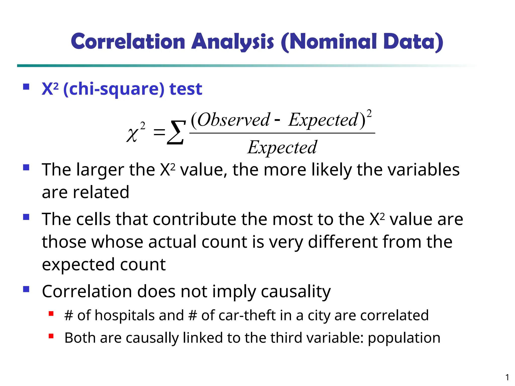
  1 Correlation Analysis (NominalData)  Χ2 (chi-square) test  The larger the Χ2 value, the more likely the variables are related  The cells that contribute the most to the Χ2 value are those whose actual count is very different from the expected count  Correlation does not imply causality  # of hospitals and # of car-theft in a city are correlated  Both are causally linked to the third variable: population    Expected Expected Observed 2 2 ) ( 
• 2.
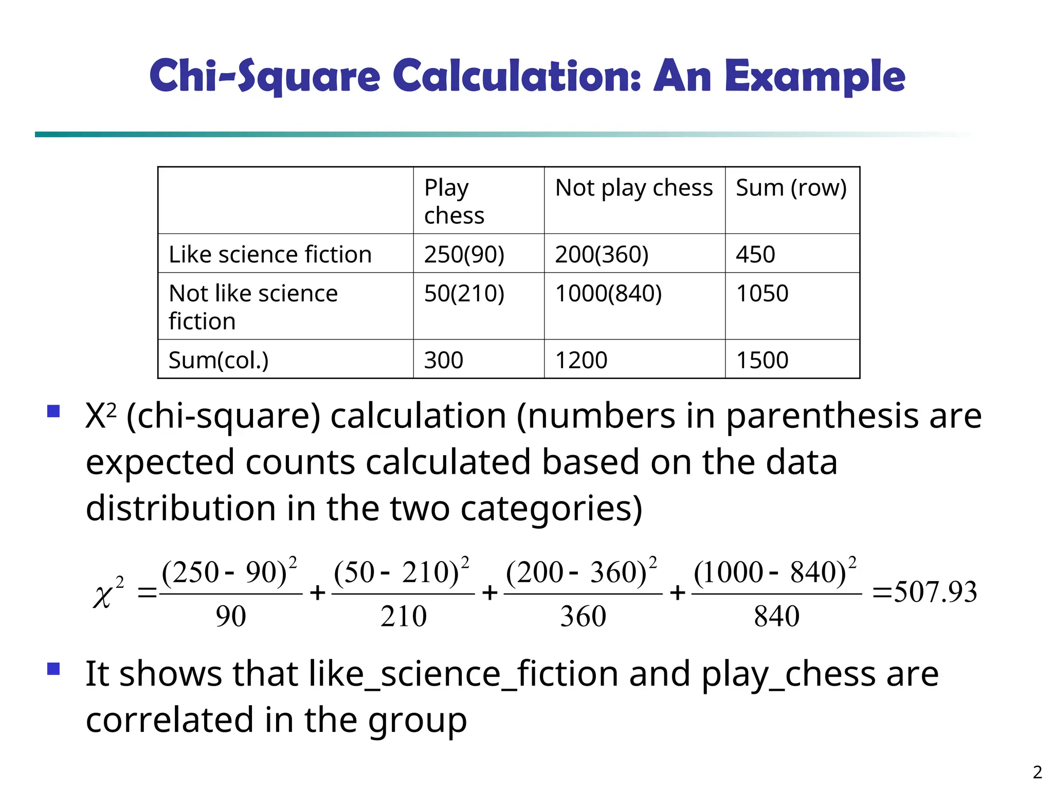
  2 Chi-Square Calculation: AnExample  Χ2 (chi-square) calculation (numbers in parenthesis are expected counts calculated based on the data distribution in the two categories)  It shows that like_science_fiction and play_chess are correlated in the group 93 . 507 840 ) 840 1000 ( 360 ) 360 200 ( 210 ) 210 50 ( 90 ) 90 250 ( 2 2 2 2 2           Play chess Not play chess Sum (row) Like science fiction 250(90) 200(360) 450 Not like science fiction 50(210) 1000(840) 1050 Sum(col.) 300 1200 1500
• 3.
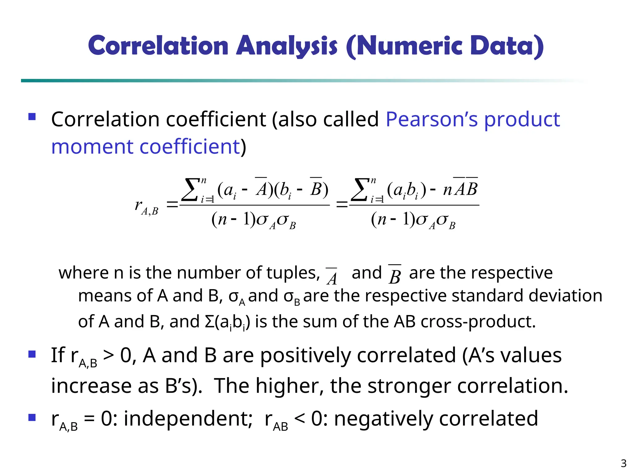
  3 Correlation Analysis (NumericData)  Correlation coefficient (also called Pearson’s product moment coefficient) where n is the number of tuples, and are the respective means of A and B, σA and σB are the respective standard deviation of A and B, and Σ(aibi) is the sum of the AB cross-product.  If rA,B > 0, A and B are positively correlated (A’s values increase as B’s). The higher, the stronger correlation.  rA,B = 0: independent; rAB < 0: negatively correlated B A n i i i B A n i i i B A n B A n b a n B b A a r     ) 1 ( ) ( ) 1 ( ) )( ( 1 1 ,            A B
• 4.
  4 Visually Evaluating Correlation Scatterplots showing the similarity from –1 to 1.
• 5.
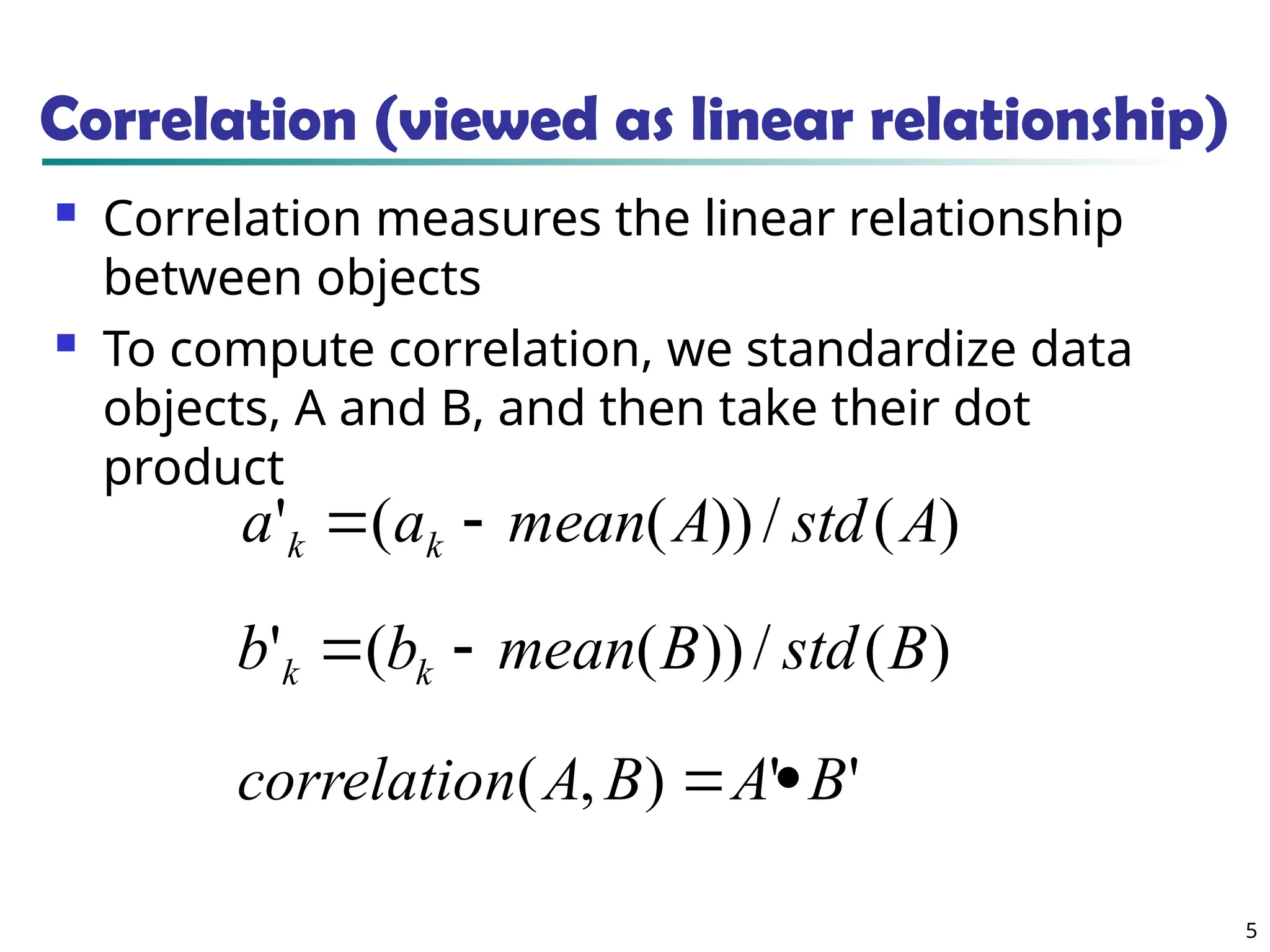
  5 Correlation (viewed aslinear relationship)  Correlation measures the linear relationship between objects  To compute correlation, we standardize data objects, A and B, and then take their dot product ) ( / )) ( ( ' A std A mean a a k k   ) ( / )) ( ( ' B std B mean b b k k   ' ' ) , ( B A B A n correlatio  
• 6.
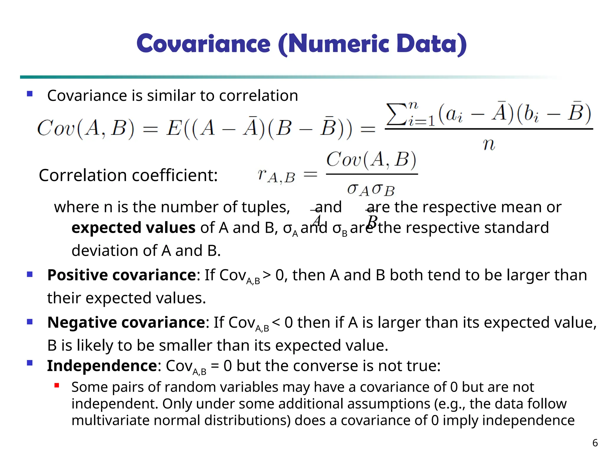
  6 Covariance (Numeric Data) Covariance is similar to correlation where n is the number of tuples, and are the respective mean or expected values of A and B, σA and σB are the respective standard deviation of A and B.  Positive covariance: If CovA,B > 0, then A and B both tend to be larger than their expected values.  Negative covariance: If CovA,B < 0 then if A is larger than its expected value, B is likely to be smaller than its expected value.  Independence: CovA,B = 0 but the converse is not true:  Some pairs of random variables may have a covariance of 0 but are not independent. Only under some additional assumptions (e.g., the data follow multivariate normal distributions) does a covariance of 0 imply independence A B Correlation coefficient:
• 7.
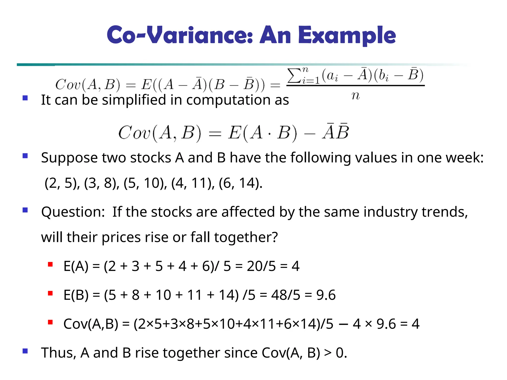
  Co-Variance: An Example It can be simplified in computation as  Suppose two stocks A and B have the following values in one week: (2, 5), (3, 8), (5, 10), (4, 11), (6, 14).  Question: If the stocks are affected by the same industry trends, will their prices rise or fall together?  E(A) = (2 + 3 + 5 + 4 + 6)/ 5 = 20/5 = 4  E(B) = (5 + 8 + 10 + 11 + 14) /5 = 48/5 = 9.6  Cov(A,B) = (2×5+3×8+5×10+4×11+6×14)/5 4 × 9.6 = 4 −  Thus, A and B rise together since Cov(A, B) > 0.
• 8.
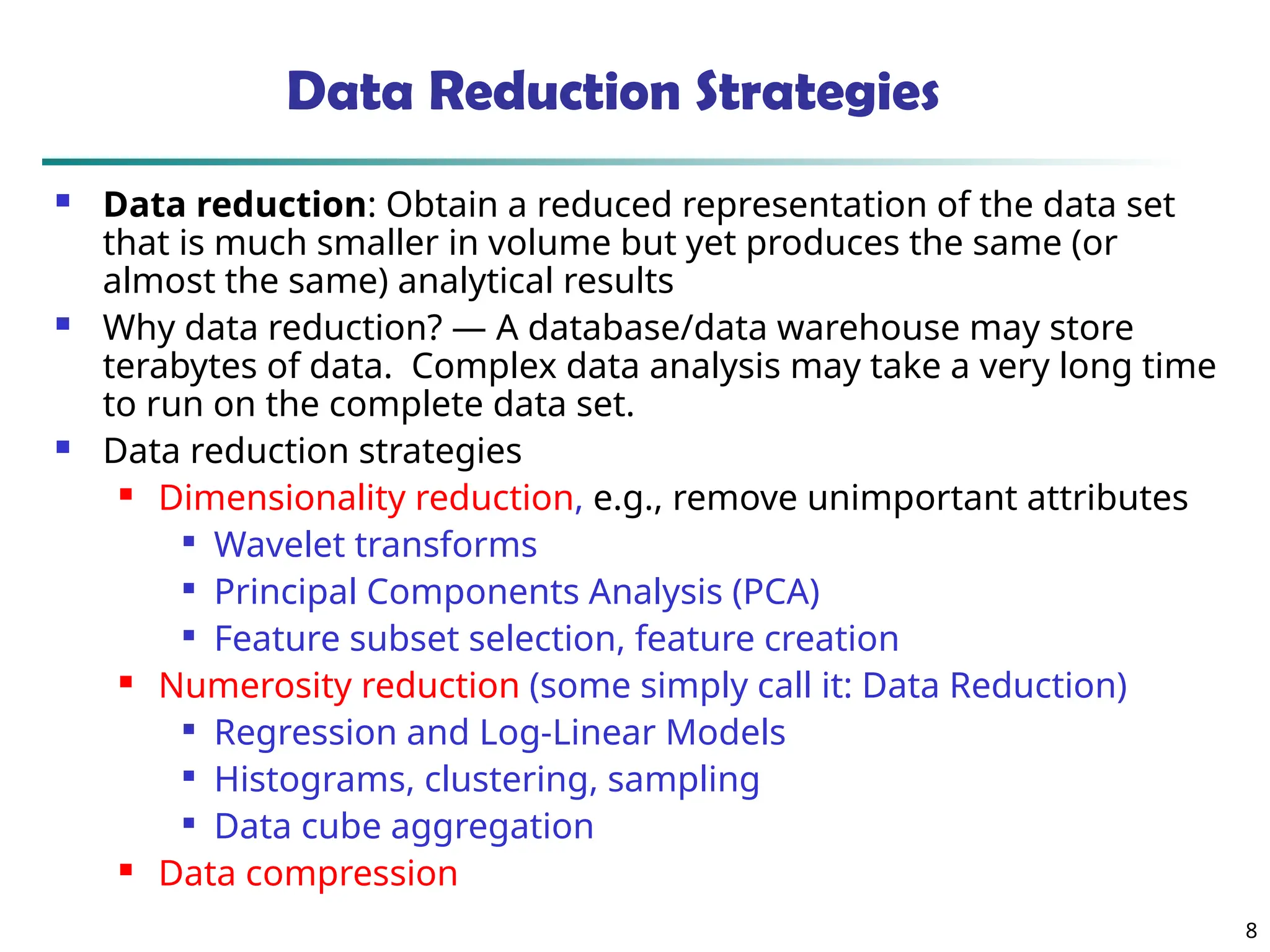
  8 Data Reduction Strategies Data reduction: Obtain a reduced representation of the data set that is much smaller in volume but yet produces the same (or almost the same) analytical results  Why data reduction? — A database/data warehouse may store terabytes of data. Complex data analysis may take a very long time to run on the complete data set.  Data reduction strategies  Dimensionality reduction, e.g., remove unimportant attributes  Wavelet transforms  Principal Components Analysis (PCA)  Feature subset selection, feature creation  Numerosity reduction (some simply call it: Data Reduction)  Regression and Log-Linear Models  Histograms, clustering, sampling  Data cube aggregation  Data compression
• 9.
  9 Data Reduction 1:Dimensionality Reduction  Curse of dimensionality  When dimensionality increases, data becomes increasingly sparse  Density and distance between points, which is critical to clustering, outlier analysis, becomes less meaningful  The possible combinations of subspaces will grow exponentially  Dimensionality reduction  Avoid the curse of dimensionality  Help eliminate irrelevant features and reduce noise  Reduce time and space required in data mining  Allow easier visualization  Dimensionality reduction techniques  Wavelet transforms  Principal Component Analysis  Supervised and nonlinear techniques (e.g., feature selection)
• 10.
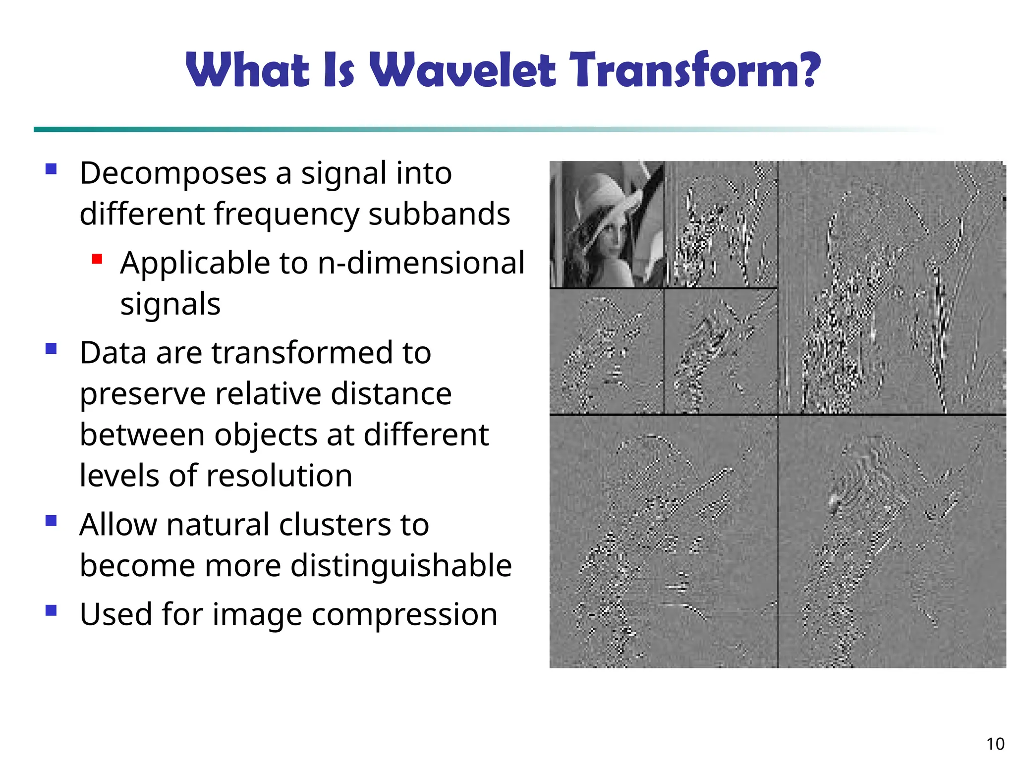
  10 What Is WaveletTransform?  Decomposes a signal into different frequency subbands  Applicable to n-dimensional signals  Data are transformed to preserve relative distance between objects at different levels of resolution  Allow natural clusters to become more distinguishable  Used for image compression