Download to read offline
![Fuzzy Set and Fuzzy Cluster Clustering methods discussed so far Every data object is assigned to exactly one cluster Some applications may need for fuzzy or soft cluster assignment Ex. An e-game could belong to both entertainment and software Methods: fuzzy clusters and probabilistic model-based clusters Fuzzy cluster: A fuzzy set S: FS : X → [0, 1] (value between 0 and 1) Example: Popularity of cameras is defined as a fuzzy mapping Then, A(0.05), B(1), C(0.86), D(0.27) 15](https://image.slidesharecdn.com/chapter11-230924172519-7a097350/75/Chapter-11-Cluster-Analysis-Advanced-Methods-ppt-15-2048.jpg)
![Fuzzy (Soft) Clustering Example: Let cluster features be C1 :“digital camera” and “lens” C2: “computer“ Fuzzy clustering k fuzzy clusters C1, …,Ck ,represented as a partition matrix M = [wij] P1: for each object oi and cluster Cj, 0 ≤ wij ≤ 1 (fuzzy set) P2: for each object oi, , equal participation in the clustering P3: for each cluster Cj , ensures there is no empty cluster Let c1, …, ck as the center of the k clusters For an object oi, sum of the squared error (SSE), p is a parameter: For a cluster Ci, SSE: Measure how well a clustering fits the data: 16](https://image.slidesharecdn.com/chapter11-230924172519-7a097350/75/Chapter-11-Cluster-Analysis-Advanced-Methods-ppt-16-2048.jpg)

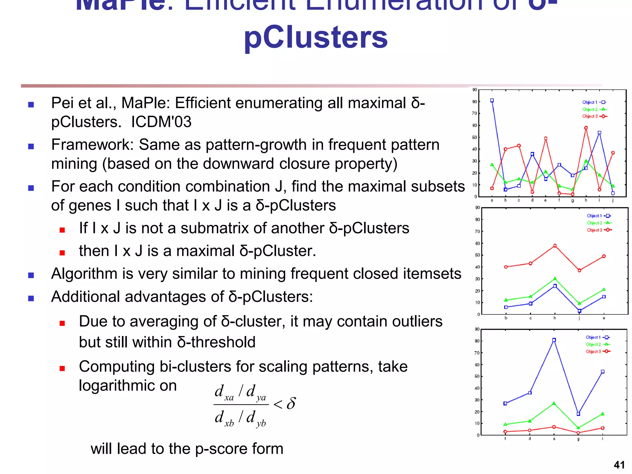
![Bi-Clustering (II): δ-pCluster Enumerating all bi-clusters (δ-pClusters) [H. Wang, et al., Clustering by pattern similarity in large data sets. SIGMOD’02] Since a submatrix I x J is a bi-cluster with (perfect) coherent values iff ei1j1 − ei2j1 = ei1j2 − ei2j2. For any 2 x 2 submatrix of I x J, define p-score A submatrix I x J is a δ-pCluster (pattern-based cluster) if the p-score of every 2 x 2 submatrix of I x J is at most δ, where δ ≥ 0 is a threshold specifying a user's tolerance of noise against a perfect bi-cluster The p-score controls the noise on every element in a bi-cluster, while the mean squared residue captures the average noise Monotonicity: If I x J is a δ-pClusters, every x x y (x,y ≥ 2) submatrix of I x J is also a δ-pClusters. A δ-pCluster is maximal if no more row or column can be added into the cluster and retain δ-pCluster: We only need to compute all maximal δ-pClusters. 40](https://image.slidesharecdn.com/chapter11-230924172519-7a097350/75/Chapter-11-Cluster-Analysis-Advanced-Methods-ppt-40-2048.jpg)
![SimRank: Similarity Based on Random Walk and Structural Context SimRank: structural-context similarity, i.e., based on the similarity of its neighbors In a directed graph G = (V,E), individual in-neighborhood of v: I(v) = {u | (u, v) ∈ E} individual out-neighborhood of v: O(v) = {w | (v, w) ∈ E} Similarity in SimRank: Initialization: Then we can compute si+1 from si based on the definition Similarity based on random walk: in a strongly connected component Expected distance: Expected meeting distance: Expected meeting probability: 48 P[t] is the probability of the tour](https://image.slidesharecdn.com/chapter11-230924172519-7a097350/75/Chapter-11-Cluster-Analysis-Advanced-Methods-ppt-48-2048.jpg)

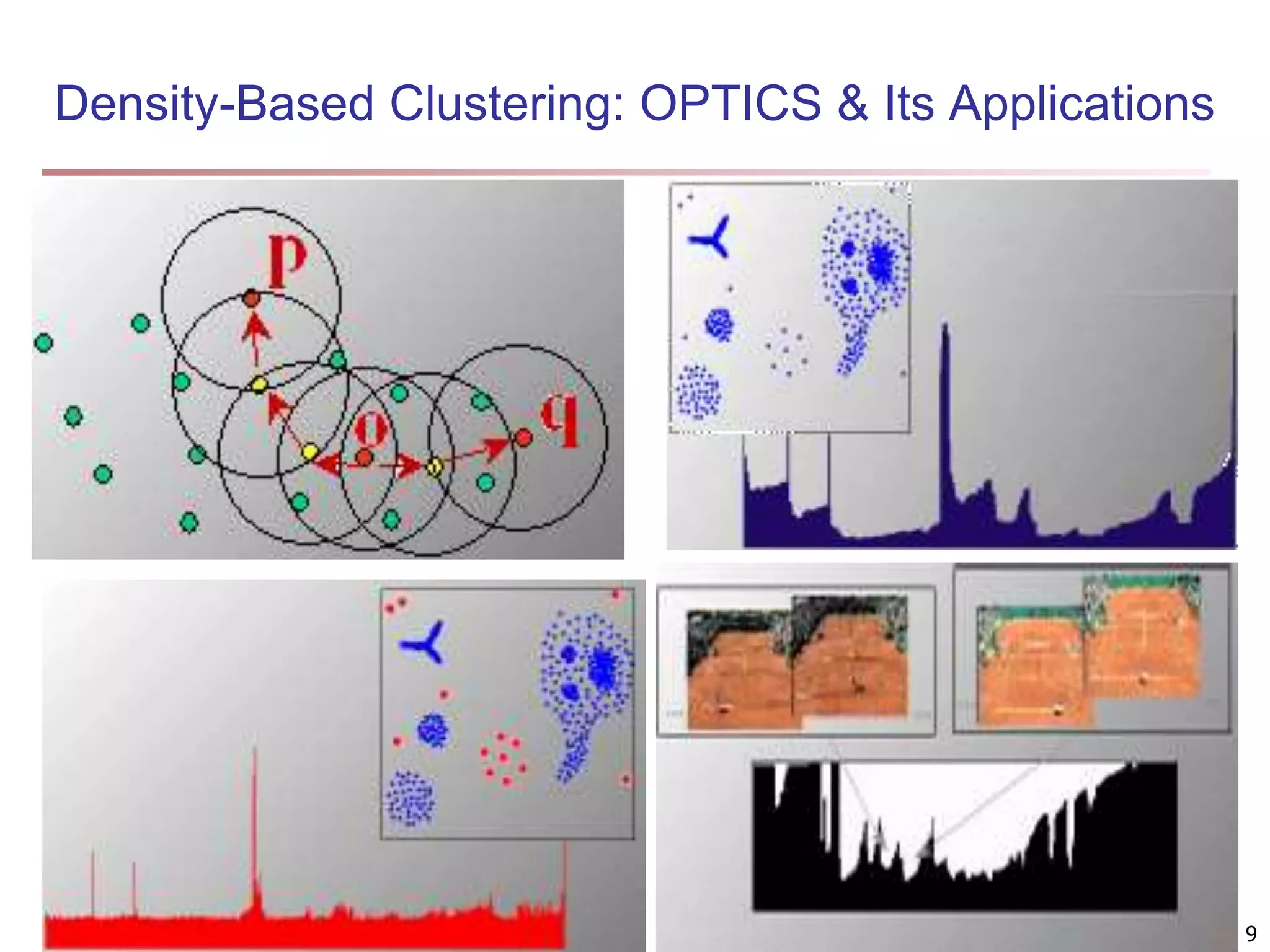
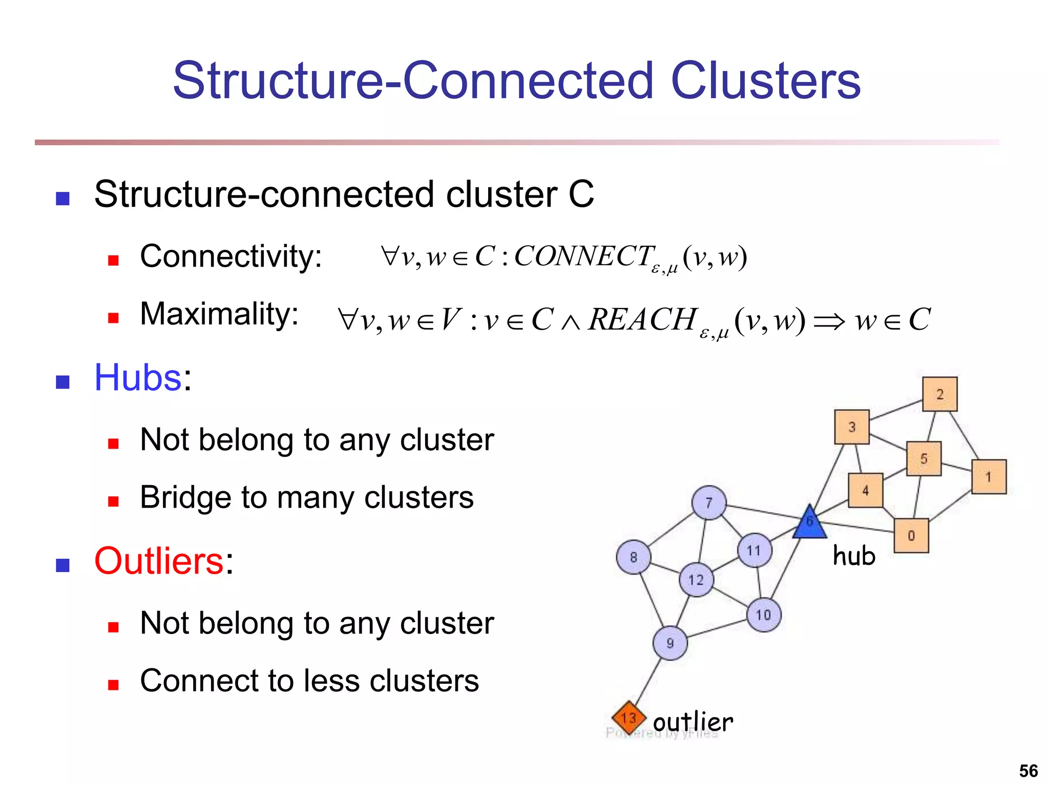
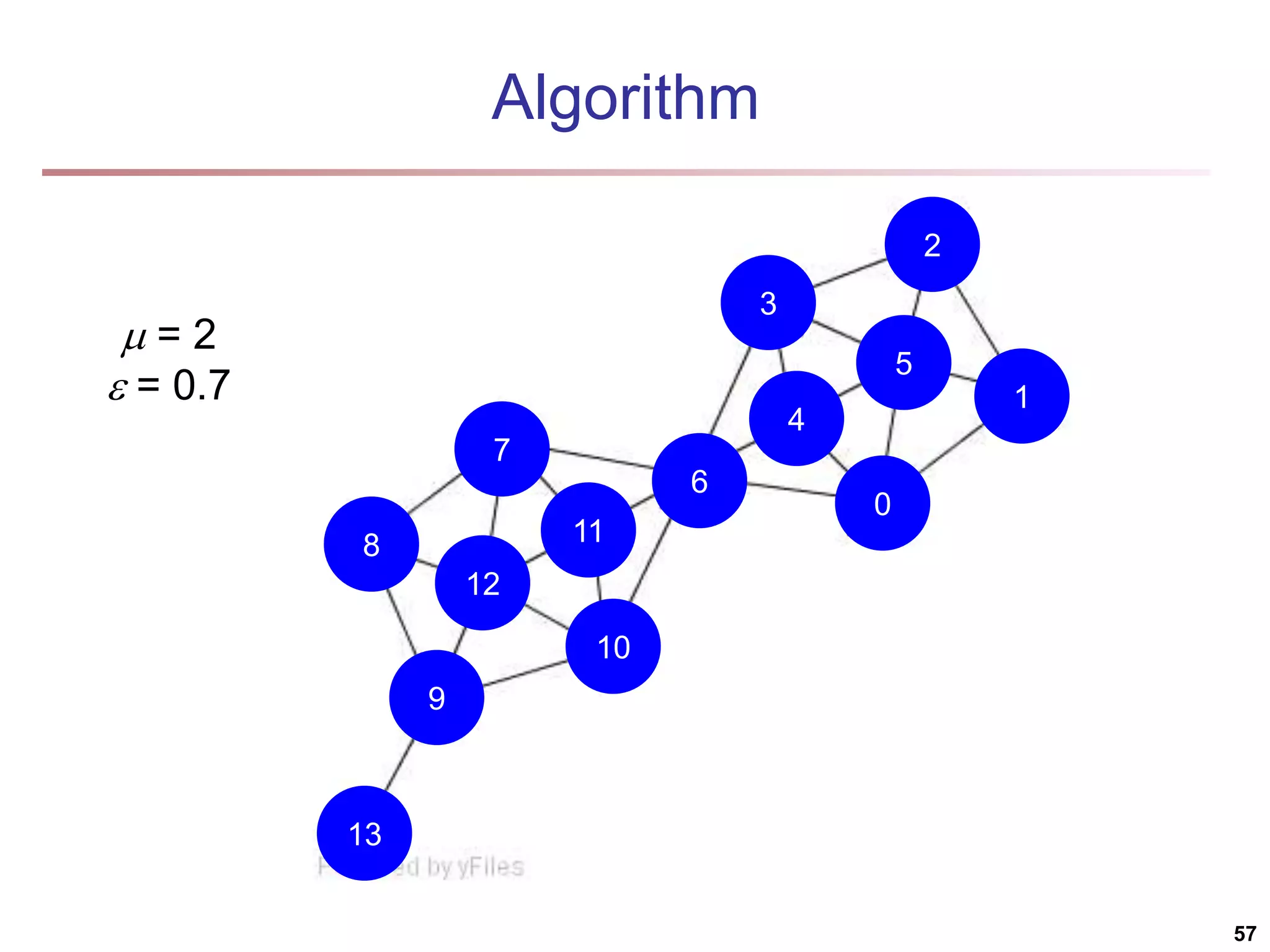
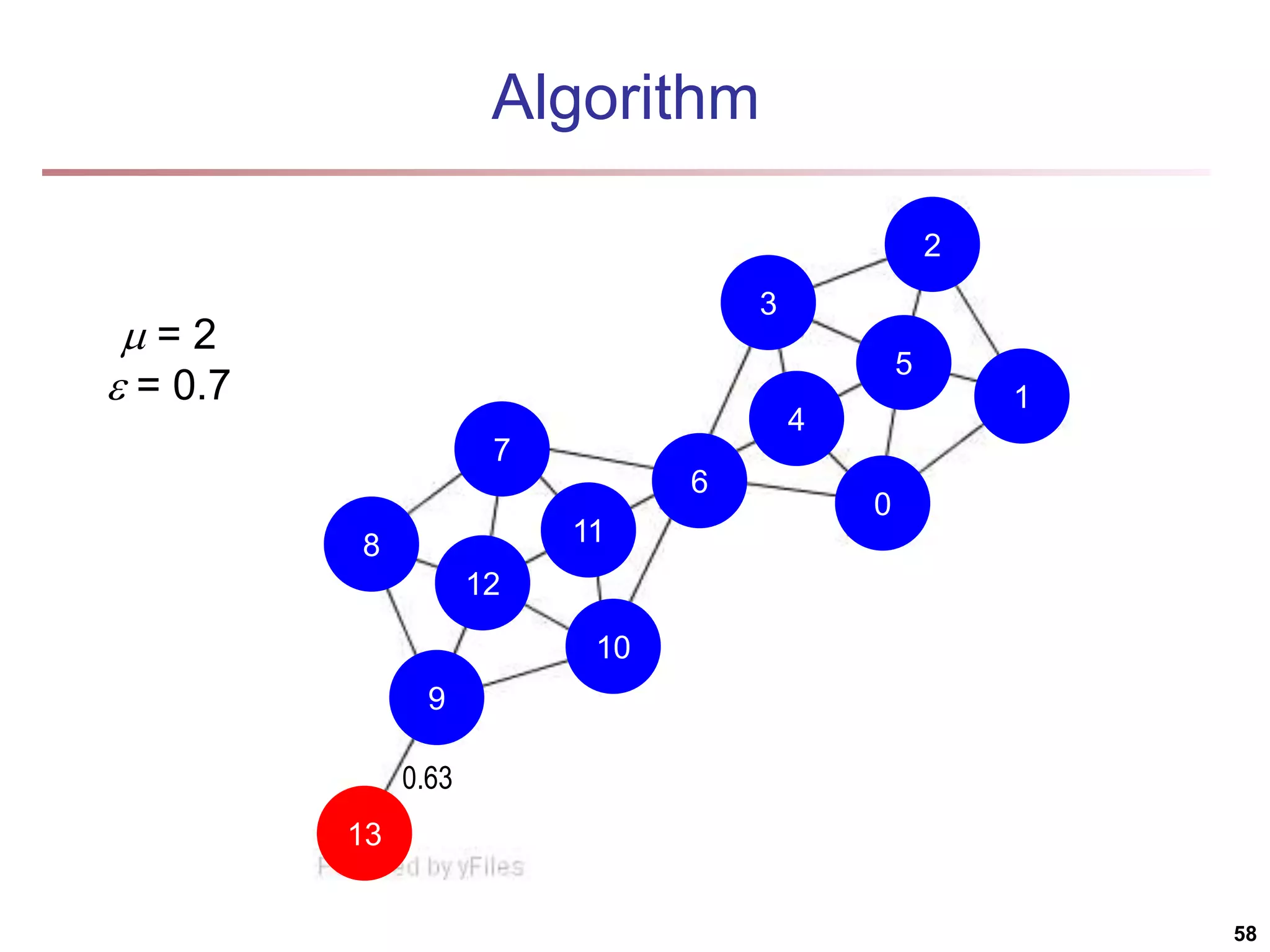
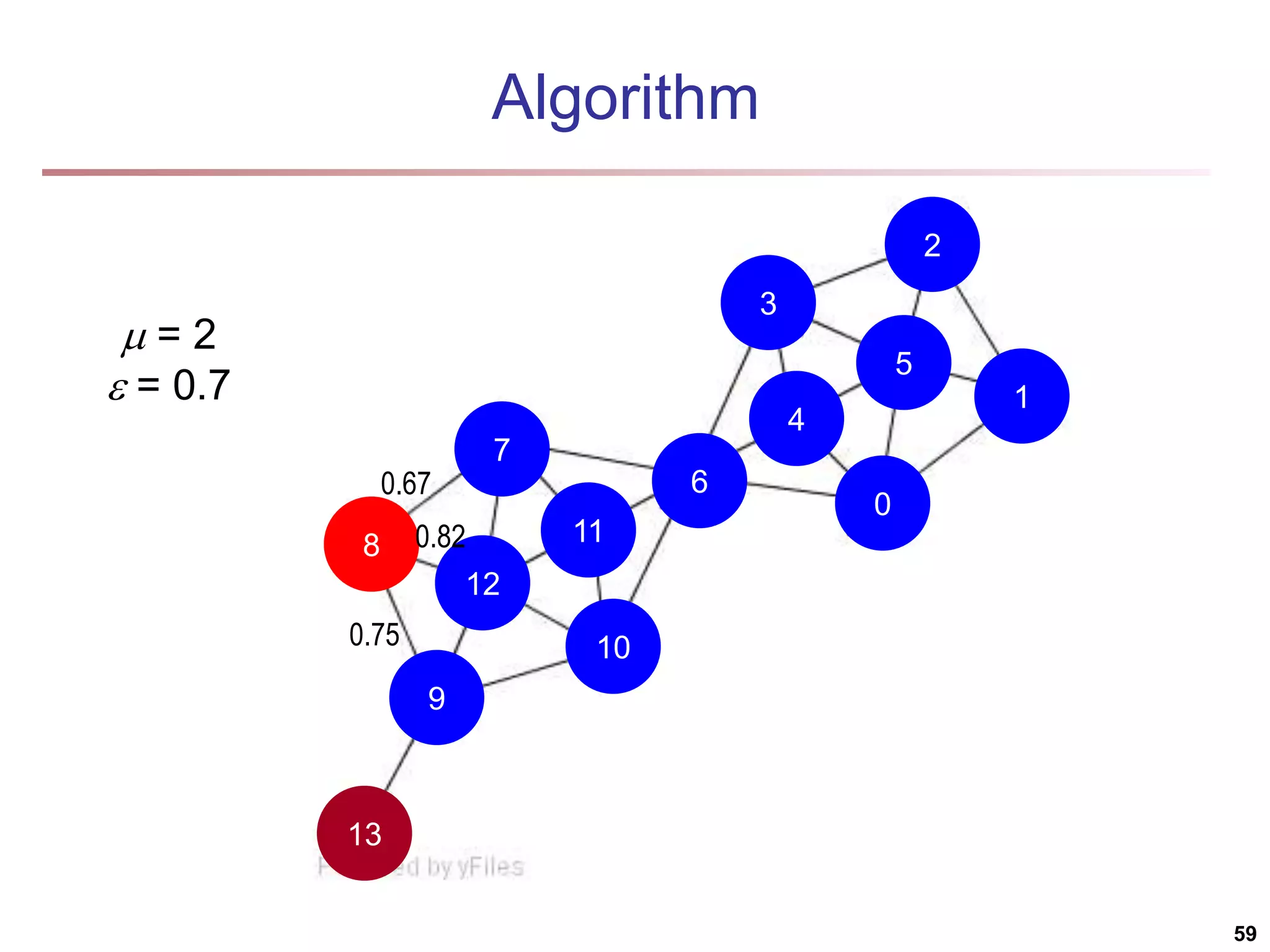
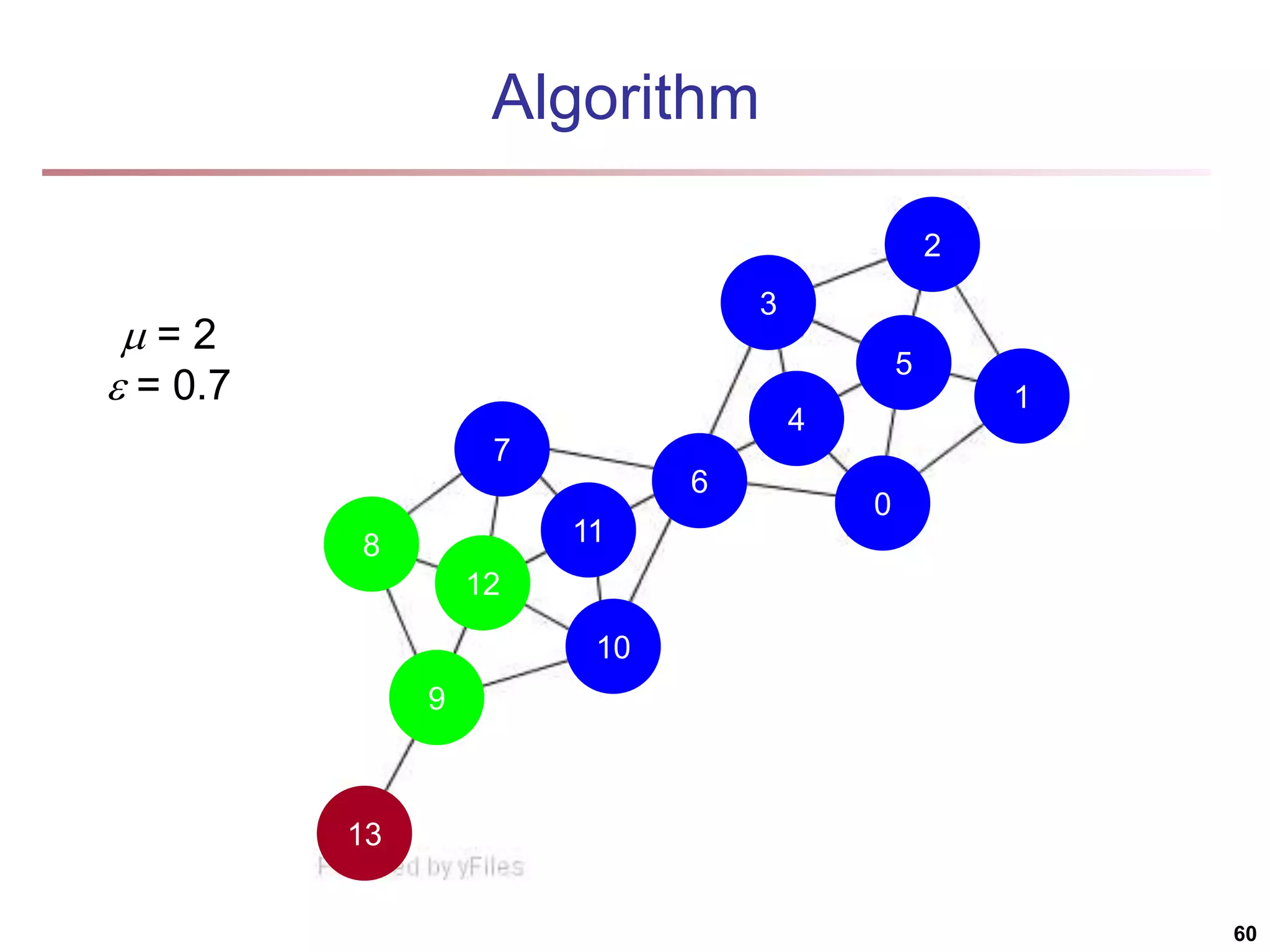
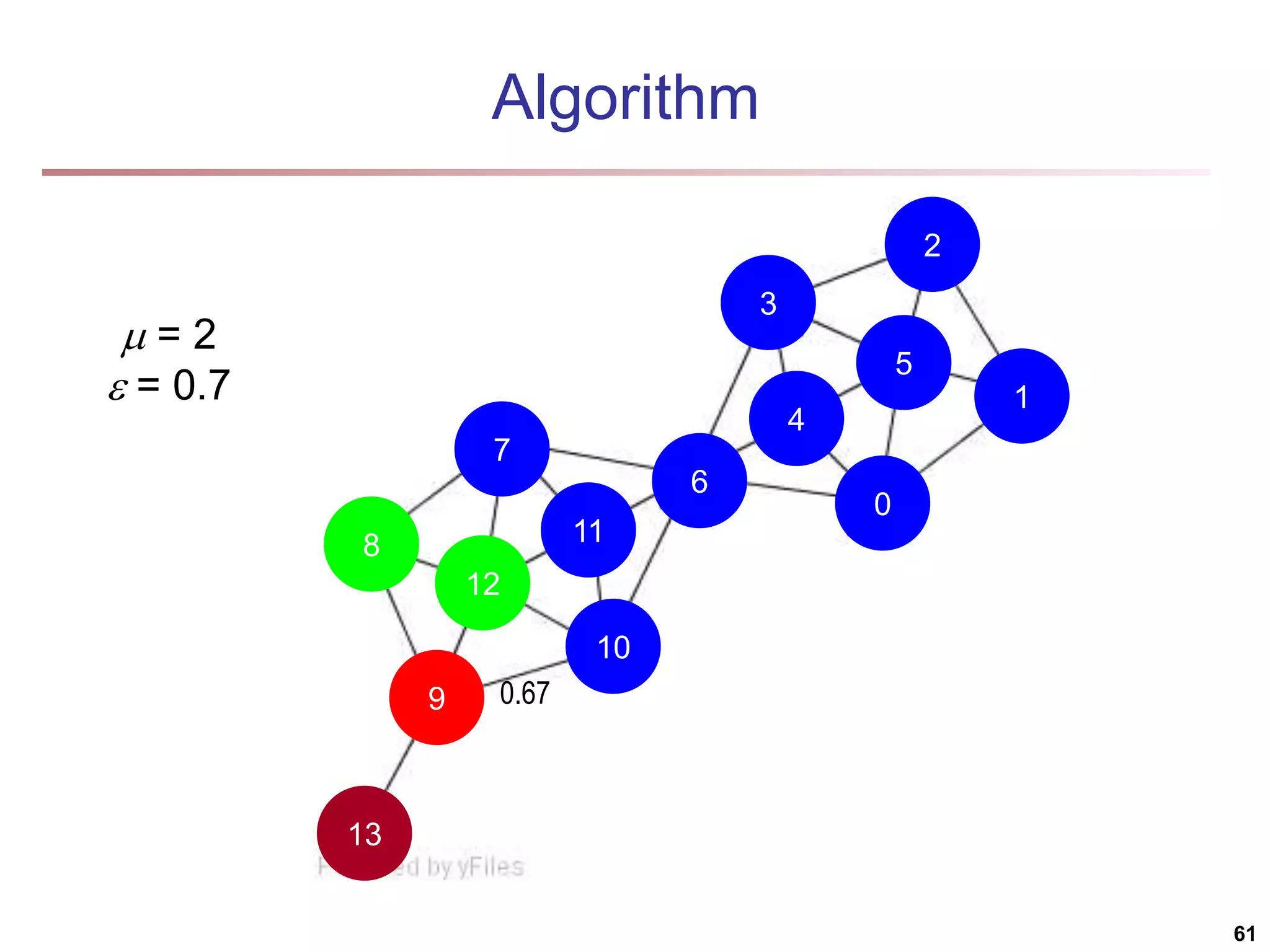
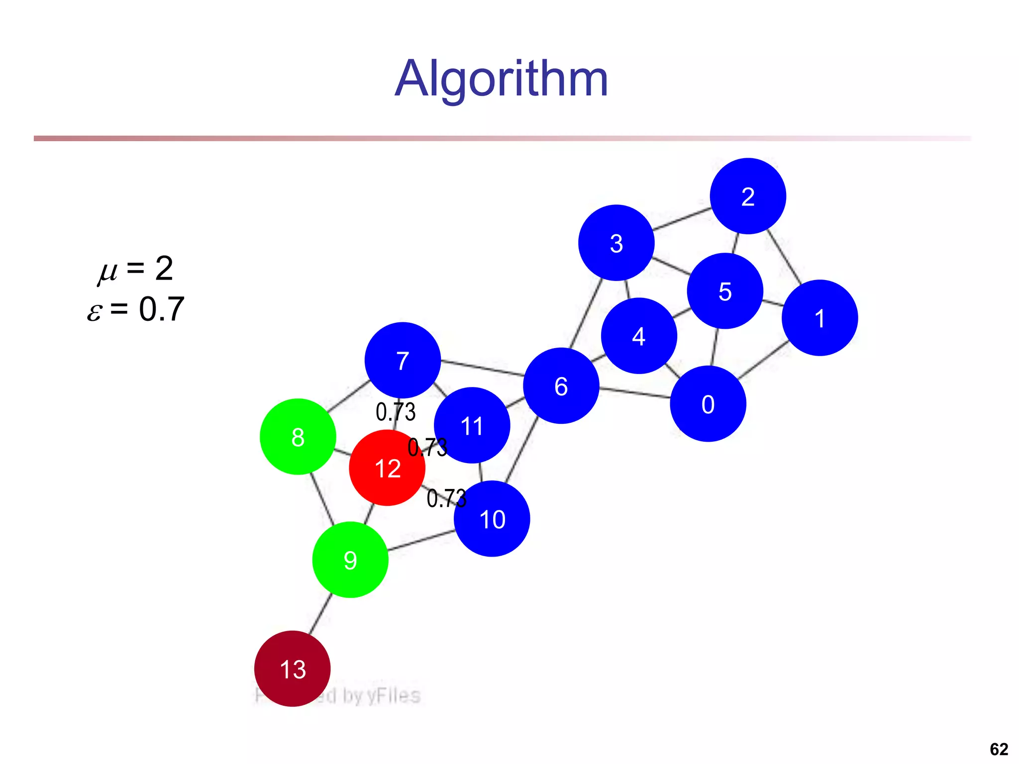
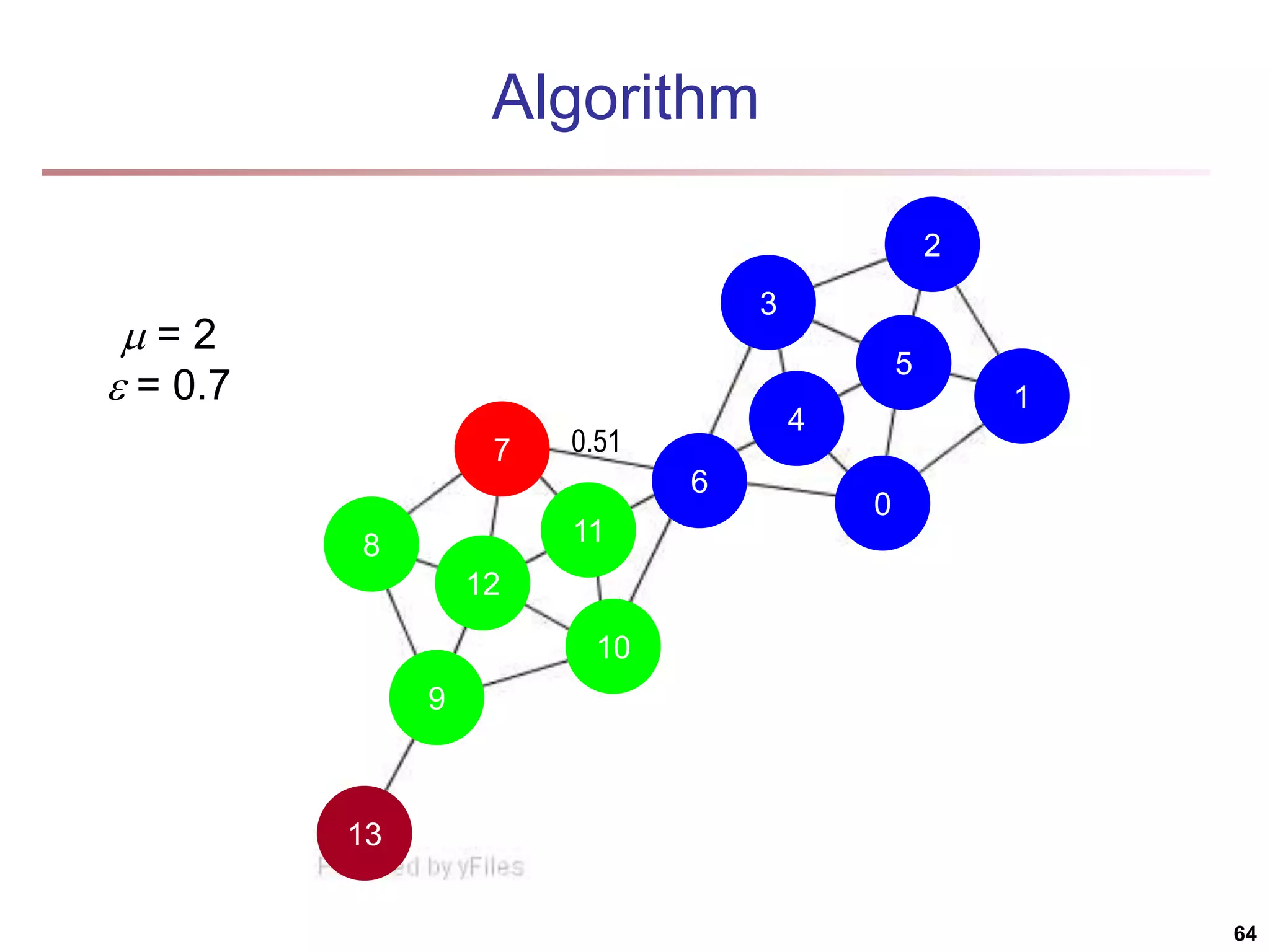
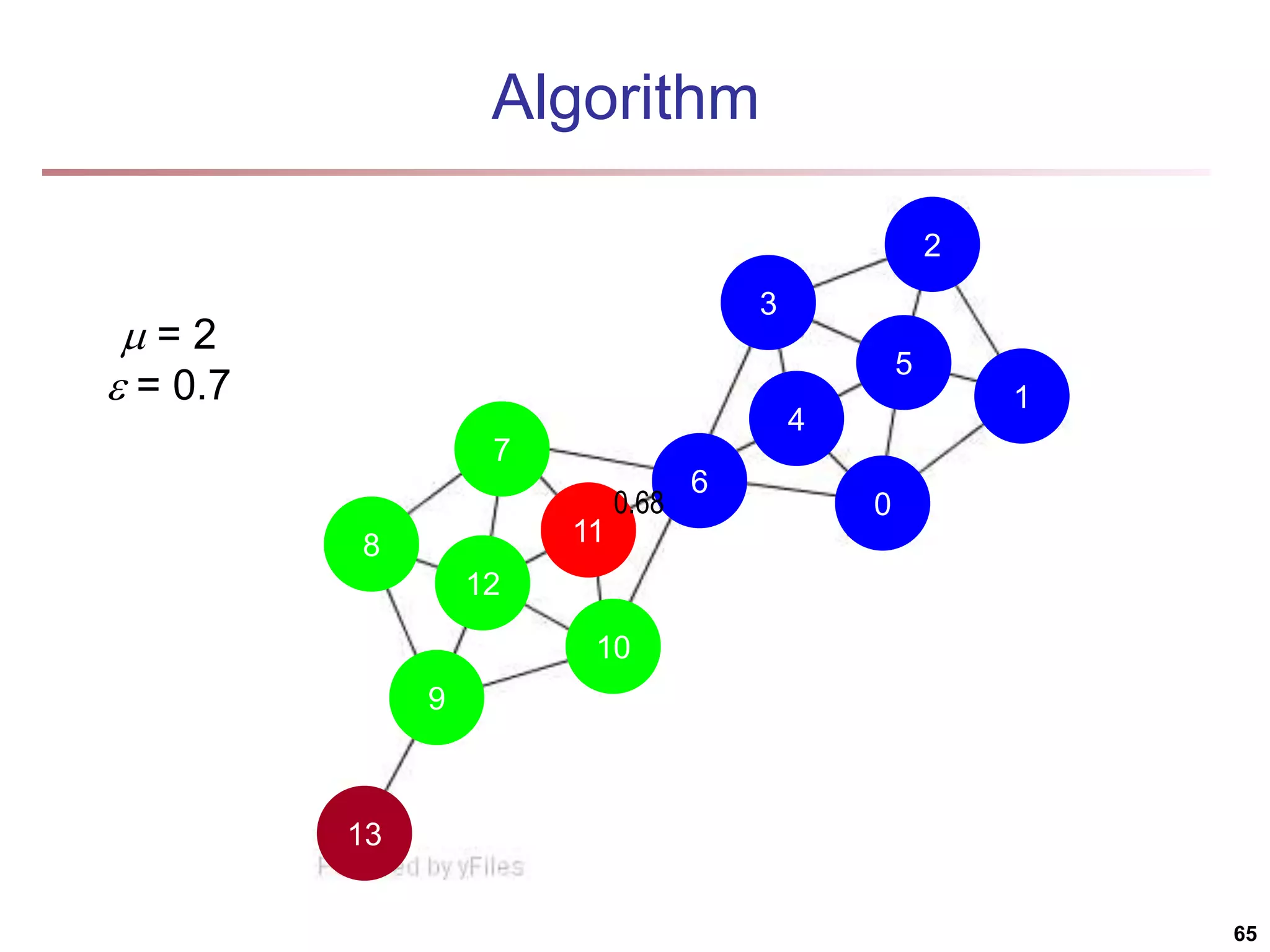
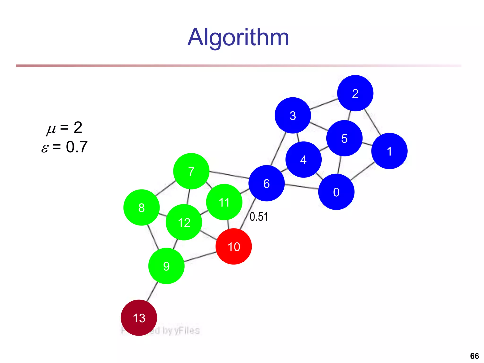
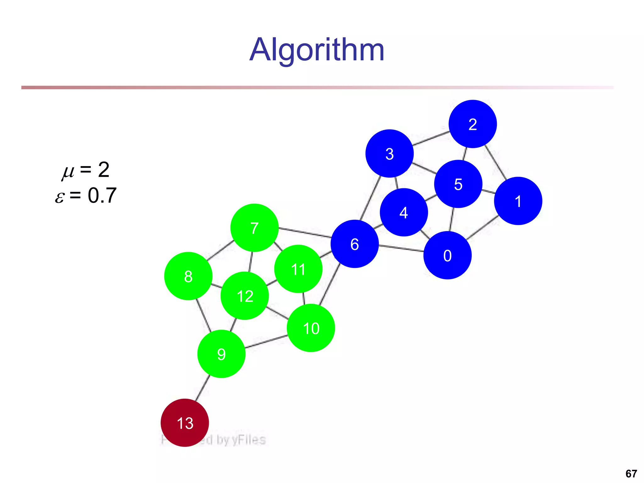
![Structural Connectivity [1] -Neighborhood: Core: Direct structure reachable: Structure reachable: transitive closure of direct structure reachability Structure connected: } ) , ( | ) ( { ) ( w v v w v N | ) ( | ) ( , v N v CORE ) ( ) ( ) , ( , , v N w v CORE w v DirRECH ) , ( ) , ( : ) , ( , , , w u RECH v u RECH V u w v CONNECT [1] M. Ester, H. P. Kriegel, J. Sander, & X. Xu (KDD'96) “A Density-Based Algorithm for Discovering Clusters in Large Spatial Databases 55](https://image.slidesharecdn.com/chapter11-230924172519-7a097350/75/Chapter-11-Cluster-Analysis-Advanced-Methods-ppt-55-2048.jpg)


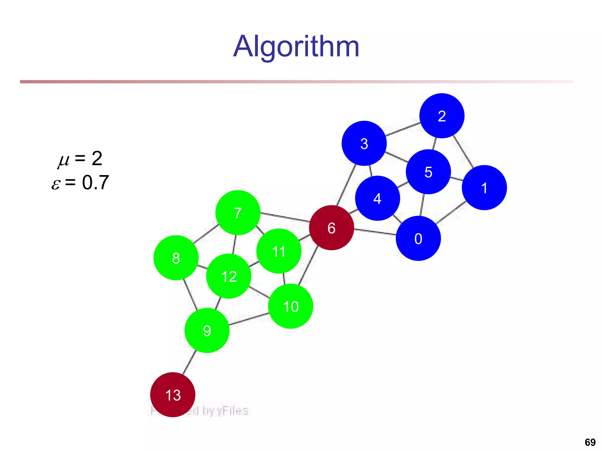
![Running Time Running time = O(|E|) For sparse networks = O(|V|) [2] A. Clauset, M. E. J. Newman, & C. Moore, Phys. Rev. E 70, 066111 (2004). 70](https://image.slidesharecdn.com/chapter11-230924172519-7a097350/75/Chapter-11-Cluster-Analysis-Advanced-Methods-ppt-70-2048.jpg)
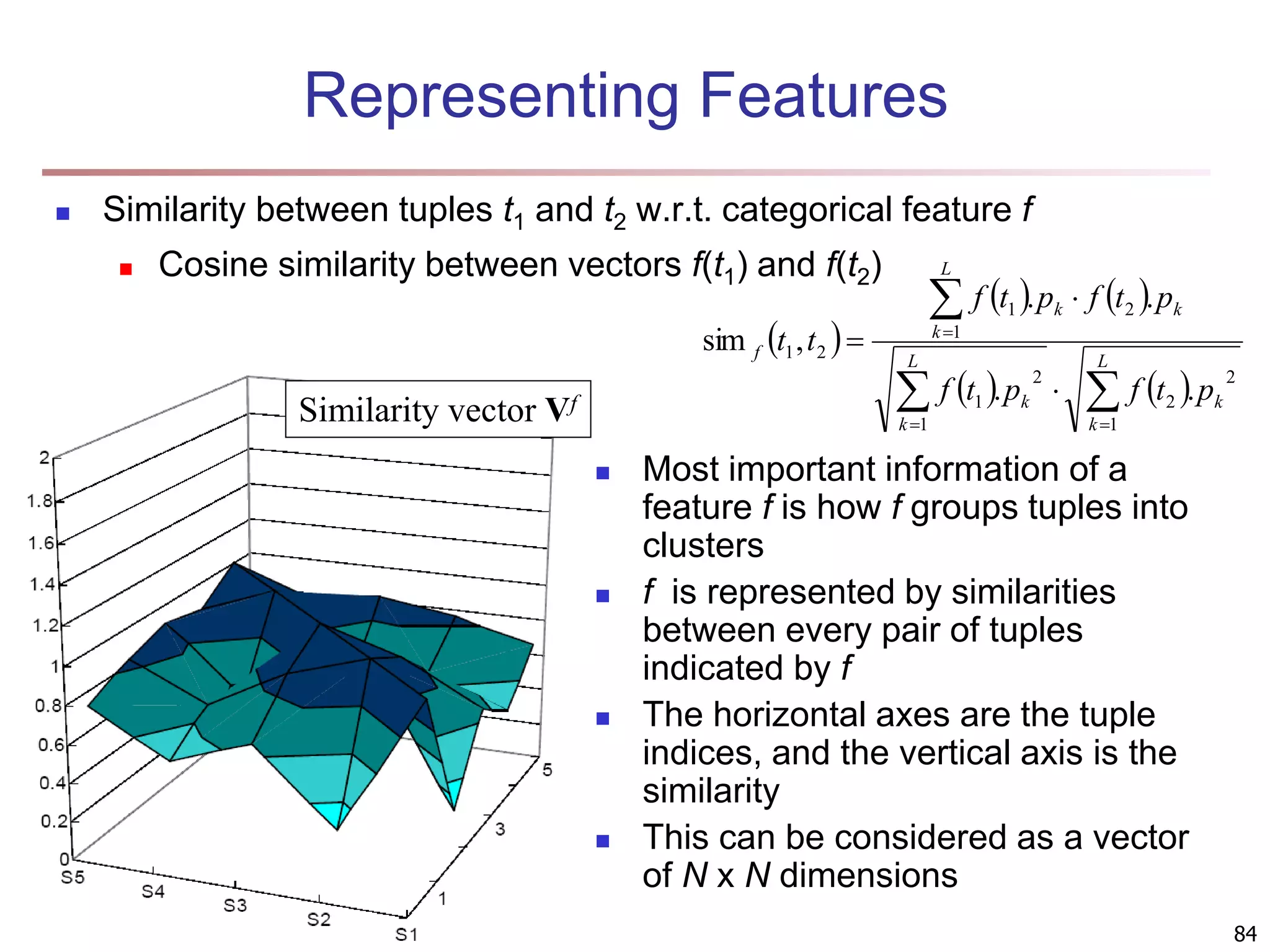
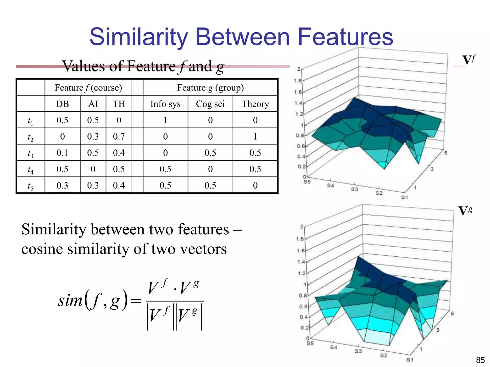
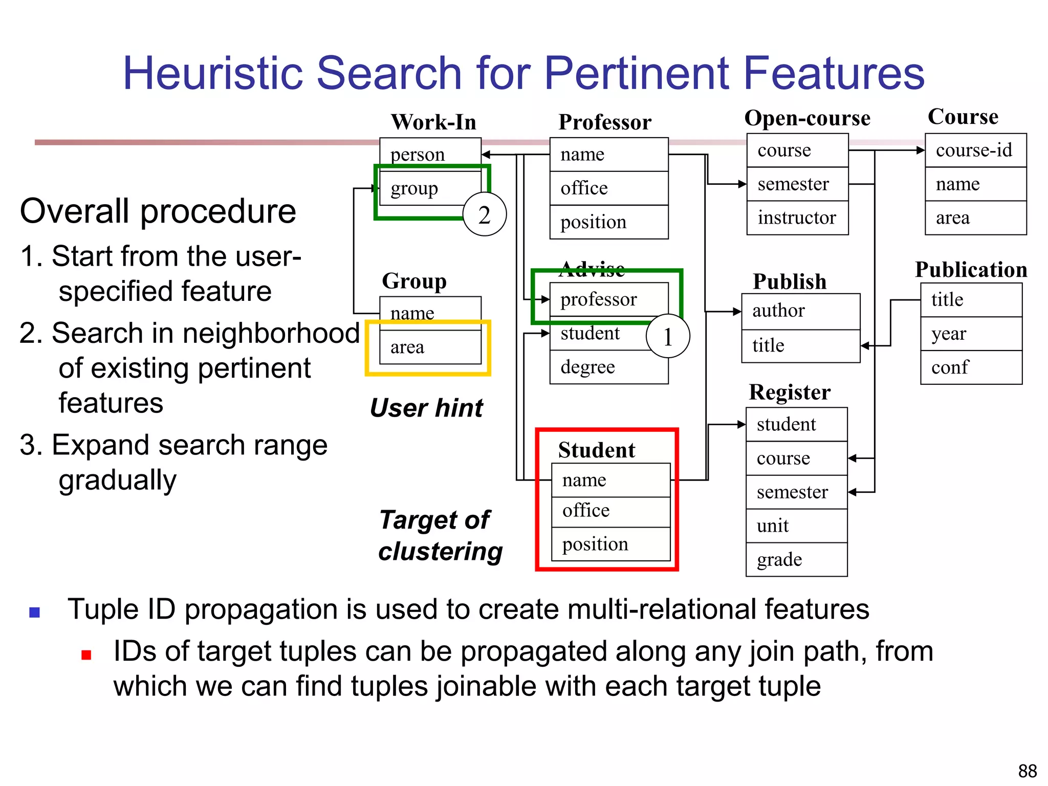
![83 Multi-Relational Features A multi-relational feature is defined by: A join path, e.g., Student → Register → OpenCourse → Course An attribute, e.g., Course.area (For numerical feature) an aggregation operator, e.g., sum or average Categorical feature f = [Student → Register → OpenCourse → Course, Course.area, null] Tuple Areas of courses DB AI TH t1 5 5 0 t2 0 3 7 t3 1 5 4 t4 5 0 5 t5 3 3 4 areas of courses of each student Tuple Feature f DB AI TH t1 0.5 0.5 0 t2 0 0.3 0.7 t3 0.1 0.5 0.4 t4 0.5 0 0.5 t5 0.3 0.3 0.4 Values of feature f f(t1) f(t2) f(t3) f(t4) f(t5) DB AI TH](https://image.slidesharecdn.com/chapter11-230924172519-7a097350/75/Chapter-11-Cluster-Analysis-Advanced-Methods-ppt-83-2048.jpg)
![89 Clustering with Multi-Relational Features Given a set of L pertinent features f1, …, fL, similarity between two tuples Weight of a feature is determined in feature search by its similarity with other pertinent features Clustering methods CLARANS [Ng & Han 94], a scalable clustering algorithm for non-Euclidean space K-means Agglomerative hierarchical clustering L i i f weight f t t t t i 1 2 1 2 1 . , sim , sim](https://image.slidesharecdn.com/chapter11-230924172519-7a097350/75/Chapter-11-Cluster-Analysis-Advanced-Methods-ppt-89-2048.jpg)
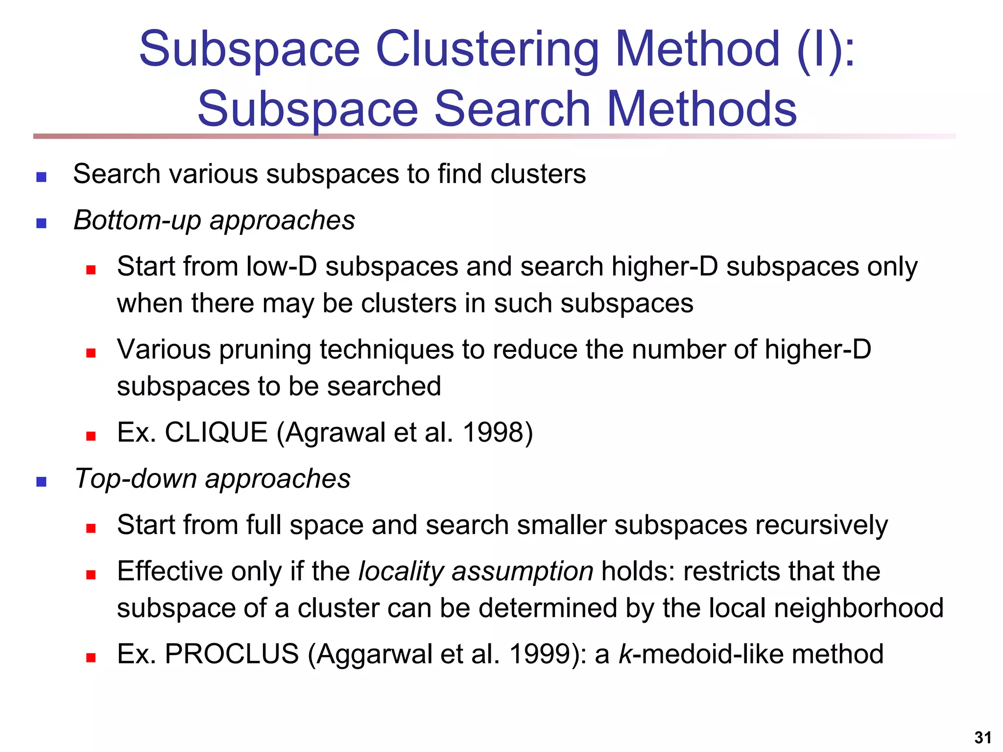
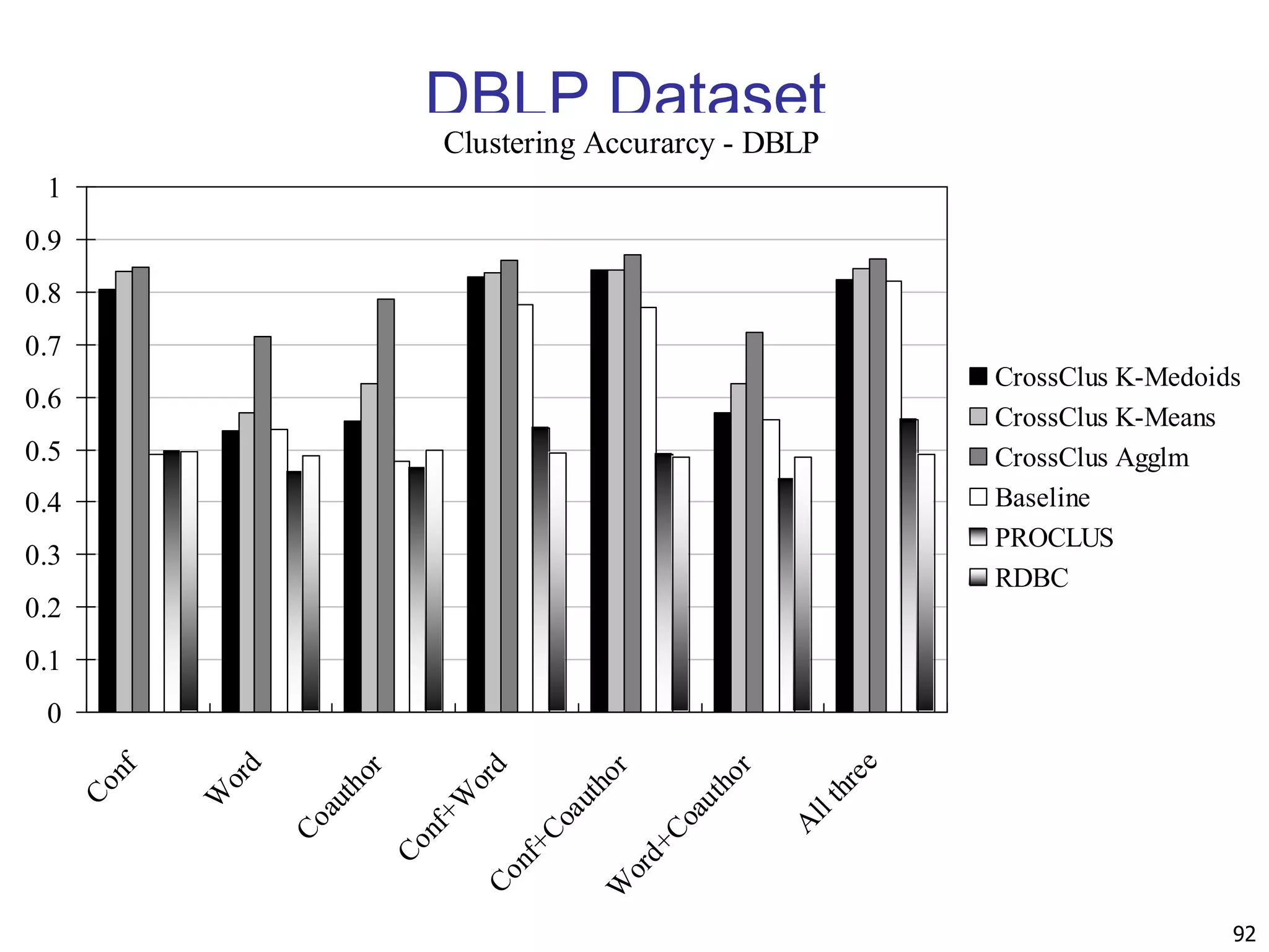
![90 Experiments: Compare CrossClus with Baseline: Only use the user specified feature PROCLUS [Aggarwal, et al. 99]: a state-of-the-art subspace clustering algorithm Use a subset of features for each cluster We convert relational database to a table by propositionalization User-specified feature is forced to be used in every cluster RDBC [Kirsten and Wrobel’00] A representative ILP clustering algorithm Use neighbor information of objects for clustering User-specified feature is forced to be used](https://image.slidesharecdn.com/chapter11-230924172519-7a097350/75/Chapter-11-Cluster-Analysis-Advanced-Methods-ppt-90-2048.jpg)

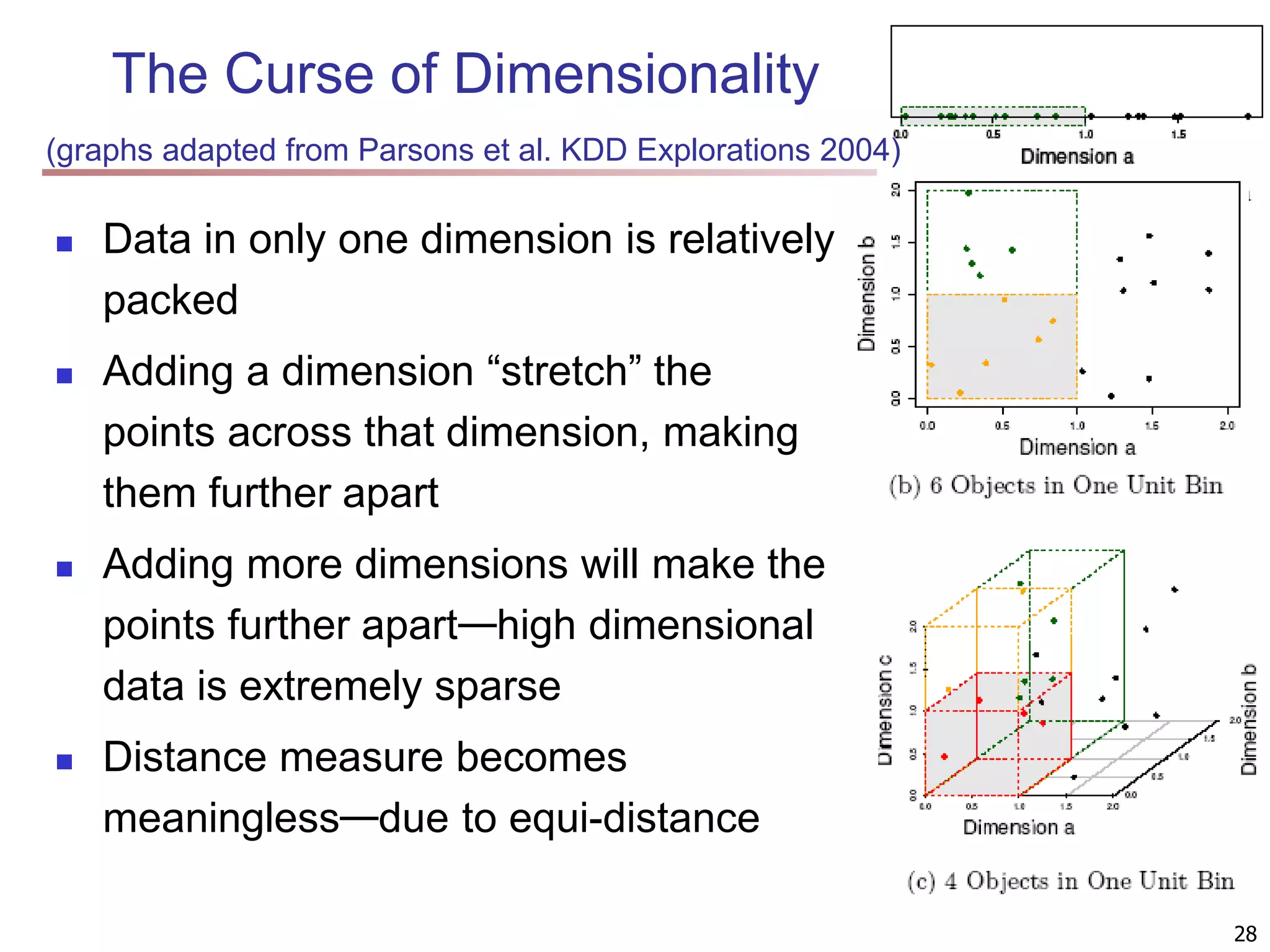
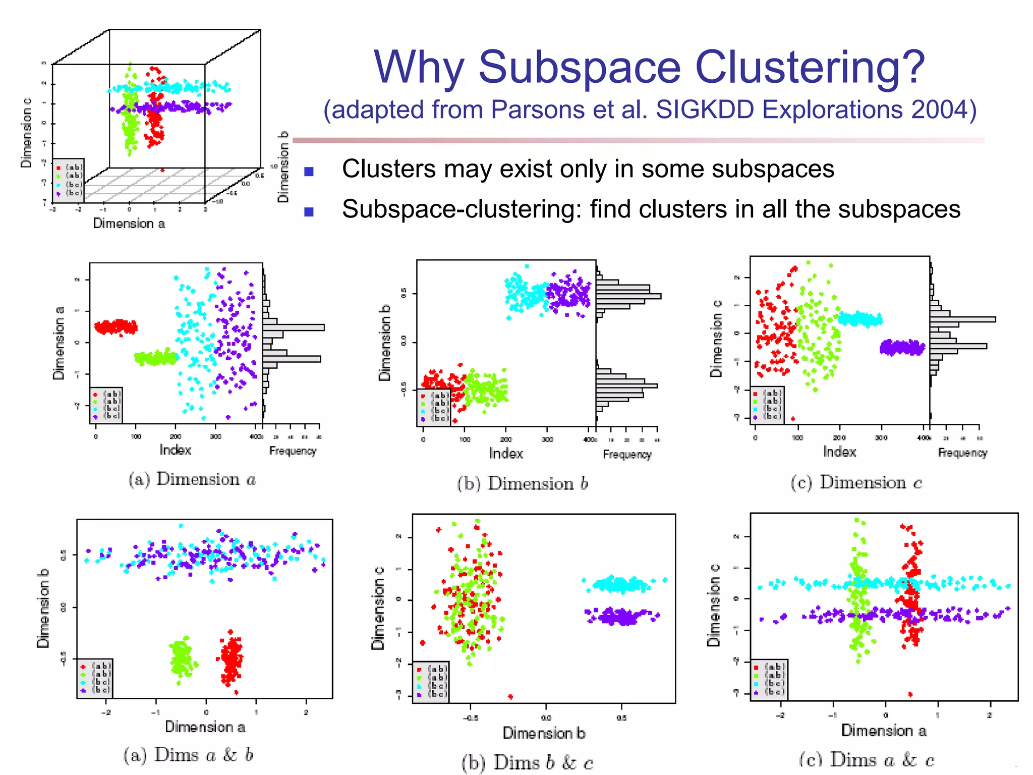
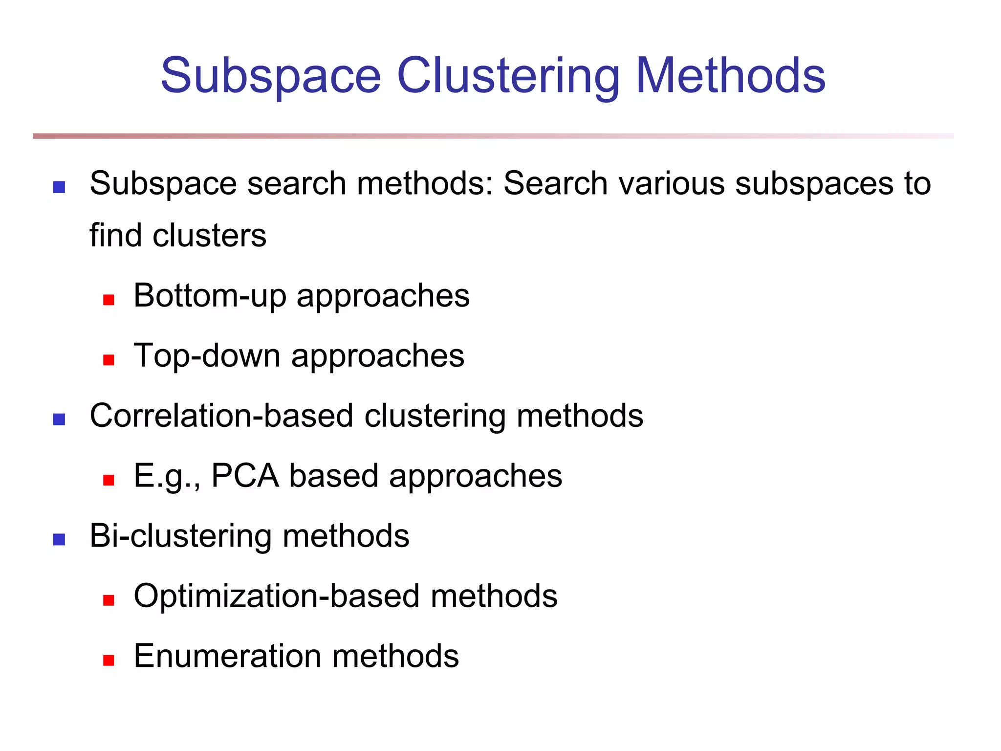
The document provides an in-depth exploration of various clustering analysis methods, including partitioning methods like k-means and hierarchical methods such as agglomerative and divisive clustering. It also discusses advanced techniques like density-based and model-based clustering approaches, addressing challenges in clustering high-dimensional data and evaluation measures for clustering quality. Additionally, it covers fuzzy clustering, subspace clustering, and bi-clustering methods, emphasizing the complexities and considerations required for effective data mining in diverse contexts.