Artificial Neural Network for machine learning

Unit - 3 Artificial Neural Networks

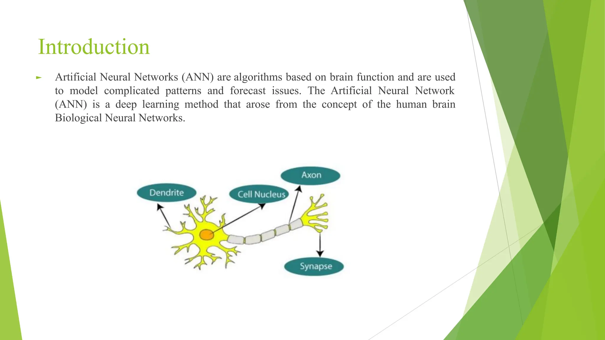
Introduction ► Artificial Neural Networks (ANN) are algorithms based on brain function and are used to model complicated patterns and forecast issues. The Artificial Neural Network (ANN) is a deep learning method that arose from the concept of the human brain Biological Neural Networks.

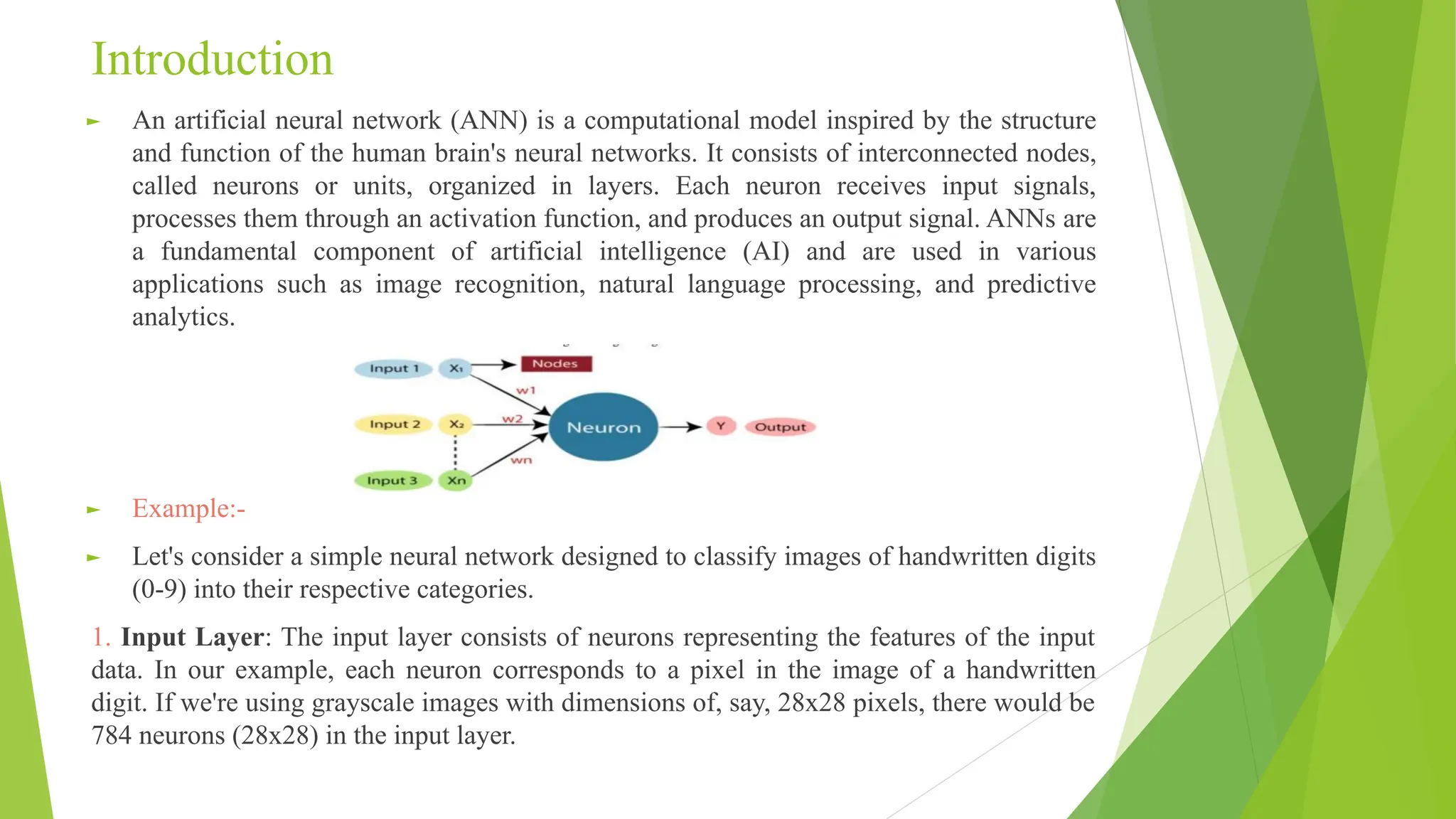
Introduction ► An artificial neural network (ANN) is a computational model inspired by the structure and function of the human brain's neural networks. It consists of interconnected nodes, called neurons or units, organized in layers. Each neuron receives input signals, processes them through an activation function, and produces an output signal. ANNs are a fundamental component of artificial intelligence (AI) and are used in various applications such as image recognition, natural language processing, and predictive analytics. ► Example:- ► Let's consider a simple neural network designed to classify images of handwritten digits (0-9) into their respective categories. 1. Input Layer: The input layer consists of neurons representing the features of the input data. In our example, each neuron corresponds to a pixel in the image of a handwritten digit. If we're using grayscale images with dimensions of, say, 28x28 pixels, there would be 784 neurons (28x28) in the input layer.

Introduction 2. Hidden Layers: Between the input and output layers, there can be one or more hidden layers. Each hidden layer contains neurons that perform computations on the input data. These layers extract features and patterns from the input data through a series of weighted connections and activation functions. The number of neurons and layers in the hidden layers is determined based on the complexity of the problem. 3.Output Layer: The output layer produces the network's predictions or classifications. In our example, it typically consists of 10 neurons, each representing one digit (0-9). The neuron with the highest output value indicates the predicted digit. 4.Weights and Bias: Each connection between neurons in adjacent layers has associated weights and a bias. These parameters are adjusted during the training process to minimize the difference between the network's predictions and the actual labels of the training data. 5.Activation Function: Each neuron applies an activation function to the weighted sum of its inputs. Common activation functions include sigmoid, tanh, ReLU (Rectified Linear Unit), and softmax. Activation functions introduce non-linearity into the network, allowing it to learn complex patterns.

Example of how the network learns: ► Training: Initially, the network's weights and biases are randomly initialized. Then, it's trained on a dataset of labeled images (e.g., the MNIST dataset). During training, the network adjusts its parameters using optimization algorithms like gradient descent to minimize the error (the difference between predicted and actual labels). ► Forward Propagation: In the forward pass, input data is fed into the network, and computations are performed layer by layer until the output is generated. ► Backpropagation: After forward propagation, the error is calculated based on the network's output and the true labels. Then, through backpropagation, this error is propagated backward through the network, and the weights and biases are adjusted accordingly using gradient descent. ► Testing: Once trained, the network is tested on a separate dataset to evaluate its performance. It can classify new, unseen images of handwritten digits into their respective categories based on the learned patterns. Through this iterative process of training and adjustment, the neural network learns to recognize patterns and make accurate predictions, demonstrating one of the fundamental capabilities of artificial intelligence.

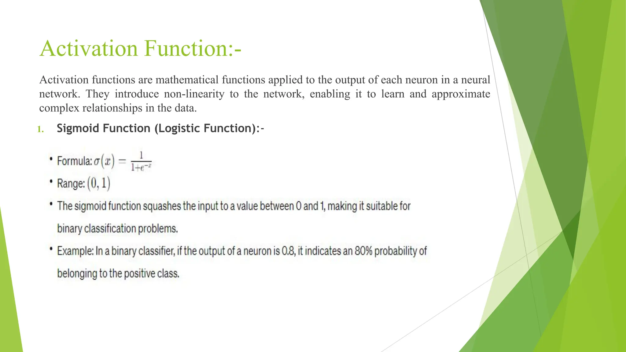
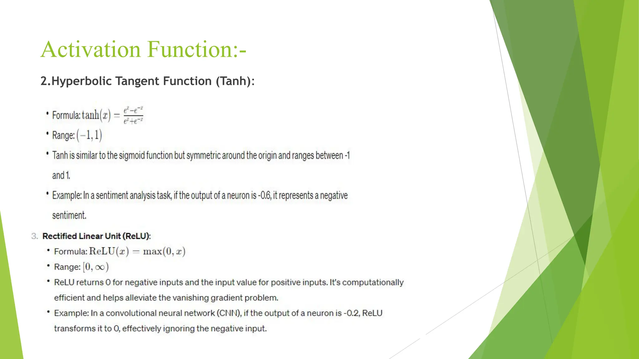
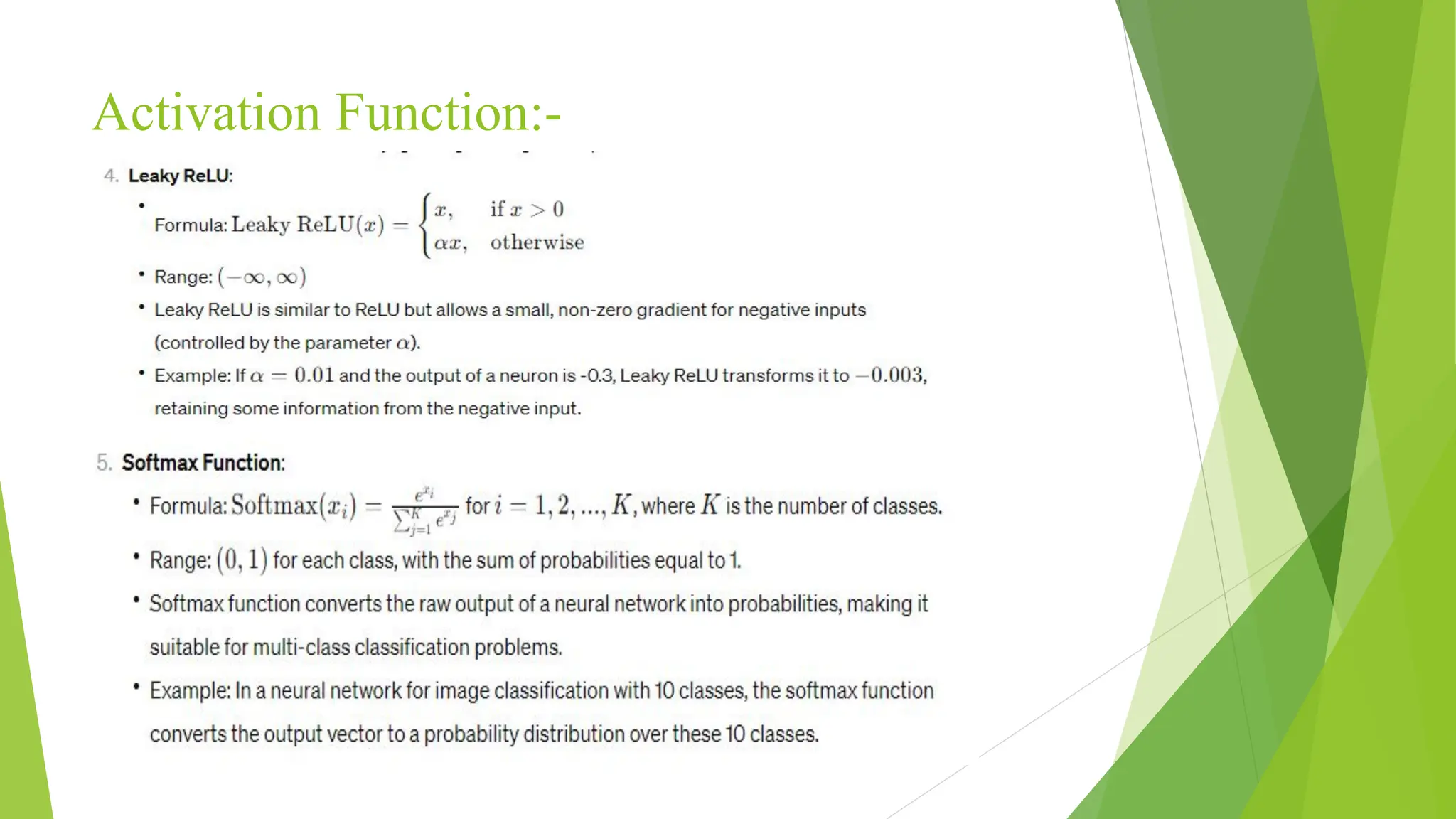
Activation Function:- Activation functions are mathematical functions applied to the output of each neuron in a neural network. They introduce non-linearity to the network, enabling it to learn and approximate complex relationships in the data. 1. Sigmoid Function (Logistic Function):-

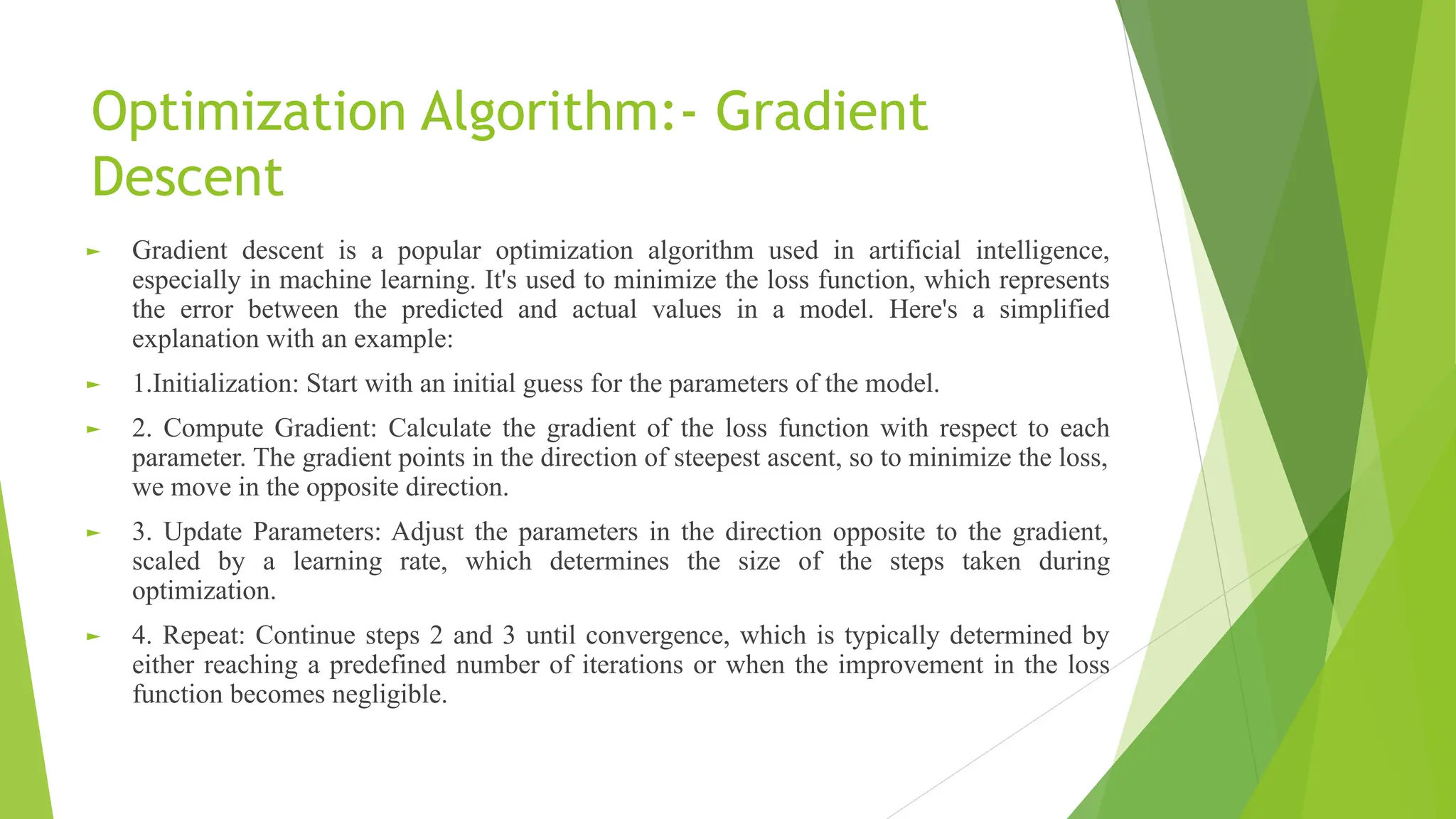
Activation Function:- 2.Hyperbolic Tangent Function (Tanh):

Optimization Algorithm:- Gradient Descent ► Gradient descent is a popular optimization algorithm used in artificial intelligence, especially in machine learning. It's used to minimize the loss function, which represents the error between the predicted and actual values in a model. Here's a simplified explanation with an example: ► 1.Initialization: Start with an initial guess for the parameters of the model. ► 2. Compute Gradient: Calculate the gradient of the loss function with respect to each parameter. The gradient points in the direction of steepest ascent, so to minimize the loss, we move in the opposite direction. ► 3. Update Parameters: Adjust the parameters in the direction opposite to the gradient, scaled by a learning rate, which determines the size of the steps taken during optimization. ► 4. Repeat: Continue steps 2 and 3 until convergence, which is typically determined by either reaching a predefined number of iterations or when the improvement in the loss function becomes negligible.

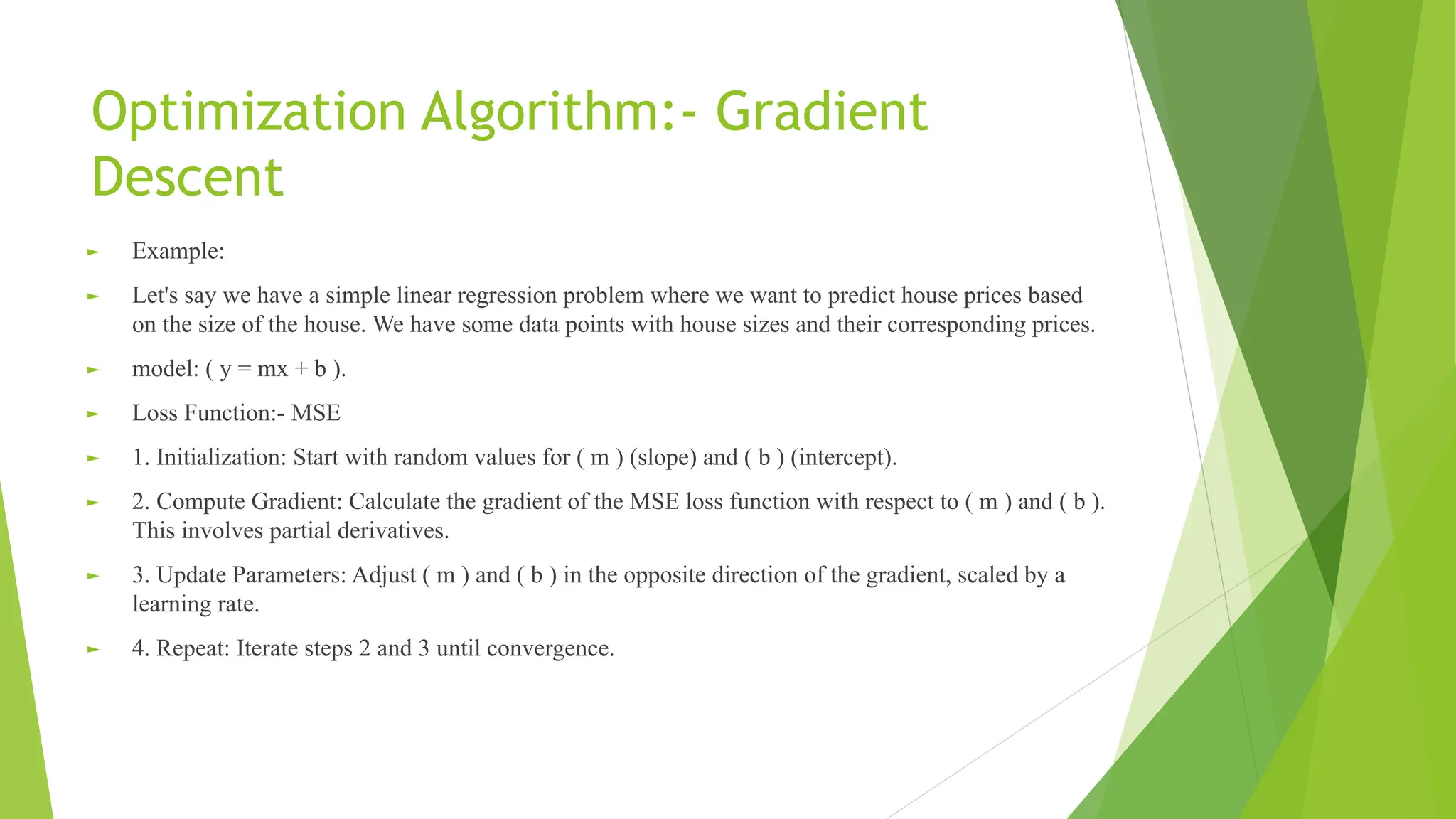
Optimization Algorithm:- Gradient Descent ► Example: ► Let's say we have a simple linear regression problem where we want to predict house prices based on the size of the house. We have some data points with house sizes and their corresponding prices. ► model: ( y = mx + b ). ► Loss Function:- MSE ► 1. Initialization: Start with random values for ( m ) (slope) and ( b ) (intercept). ► 2. Compute Gradient: Calculate the gradient of the MSE loss function with respect to ( m ) and ( b ). This involves partial derivatives. ► 3. Update Parameters: Adjust ( m ) and ( b ) in the opposite direction of the gradient, scaled by a learning rate. ► 4. Repeat: Iterate steps 2 and 3 until convergence.

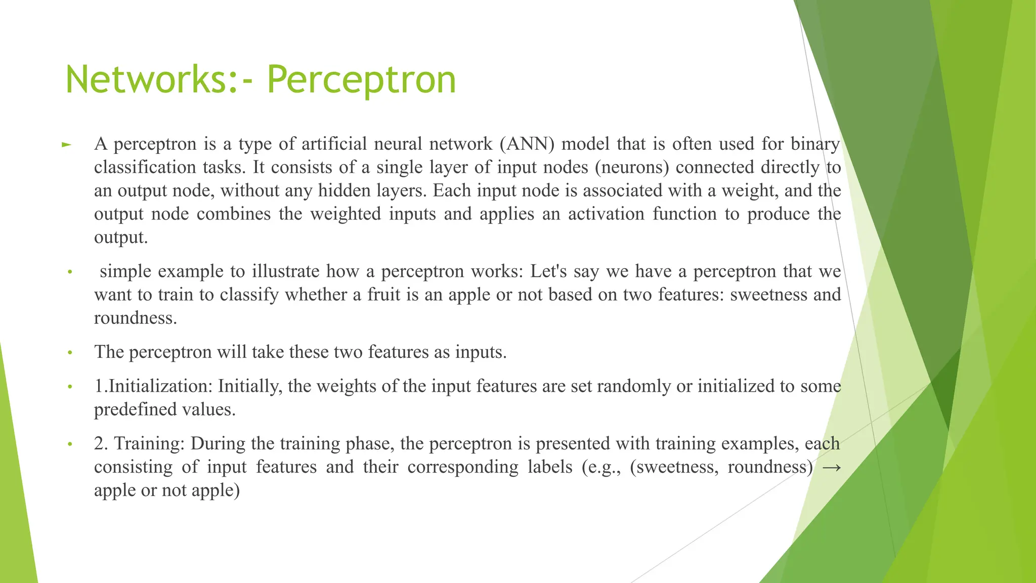
Networks:- Perceptron ► A perceptron is a type of artificial neural network (ANN) model that is often used for binary classification tasks. It consists of a single layer of input nodes (neurons) connected directly to an output node, without any hidden layers. Each input node is associated with a weight, and the output node combines the weighted inputs and applies an activation function to produce the output. • simple example to illustrate how a perceptron works: Let's say we have a perceptron that we want to train to classify whether a fruit is an apple or not based on two features: sweetness and roundness. • The perceptron will take these two features as inputs. • 1.Initialization: Initially, the weights of the input features are set randomly or initialized to some predefined values. • 2. Training: During the training phase, the perceptron is presented with training examples, each consisting of input features and their corresponding labels (e.g., (sweetness, roundness) → apple or not apple)

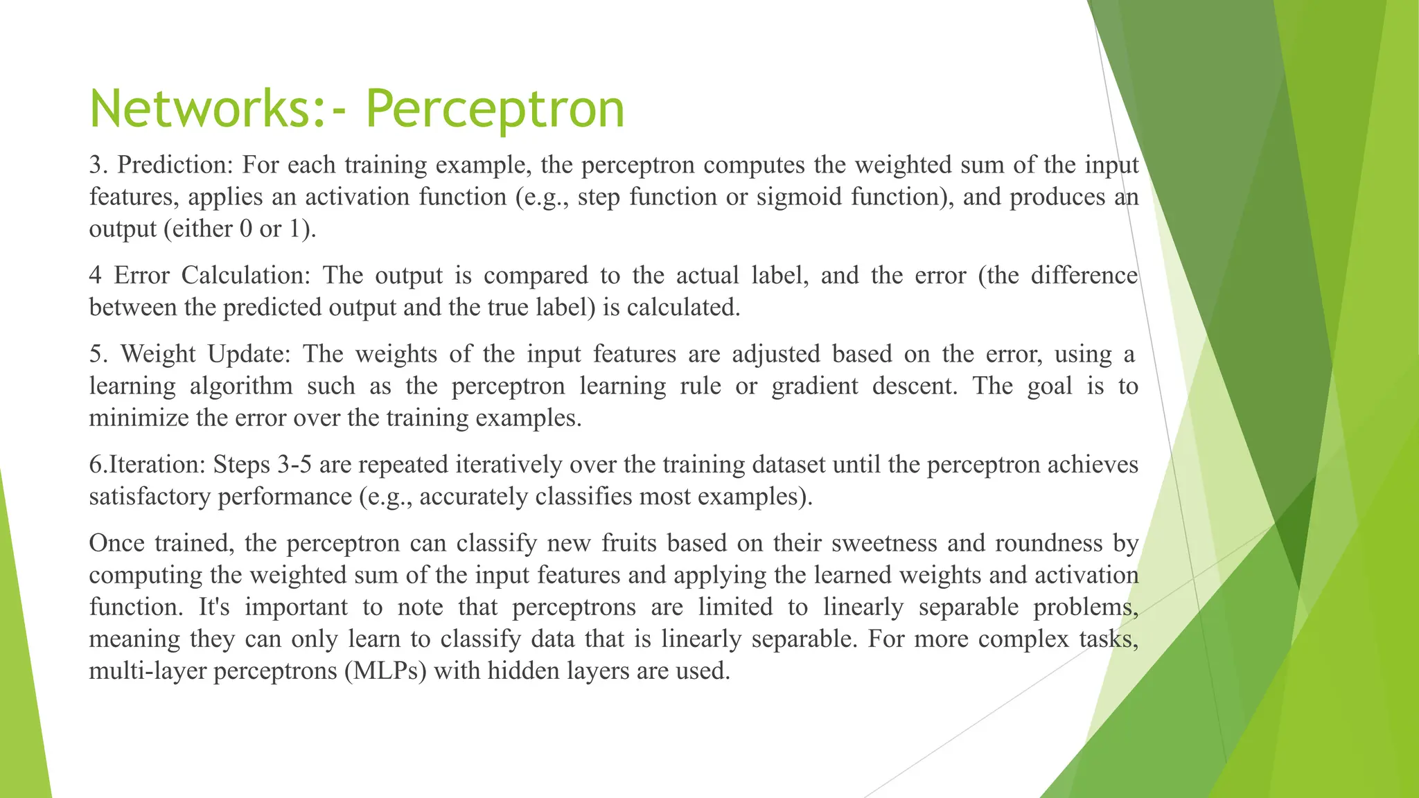
Networks:- Perceptron 3. Prediction: For each training example, the perceptron computes the weighted sum of the input features, applies an activation function (e.g., step function or sigmoid function), and produces an output (either 0 or 1). 4 Error Calculation: The output is compared to the actual label, and the error (the difference between the predicted output and the true label) is calculated. 5. Weight Update: The weights of the input features are adjusted based on the error, using a learning algorithm such as the perceptron learning rule or gradient descent. The goal is to minimize the error over the training examples. 6.Iteration: Steps 3-5 are repeated iteratively over the training dataset until the perceptron achieves satisfactory performance (e.g., accurately classifies most examples). Once trained, the perceptron can classify new fruits based on their sweetness and roundness by computing the weighted sum of the input features and applying the learned weights and activation function. It's important to note that perceptrons are limited to linearly separable problems, meaning they can only learn to classify data that is linearly separable. For more complex tasks, multi-layer perceptrons (MLPs) with hidden layers are used.

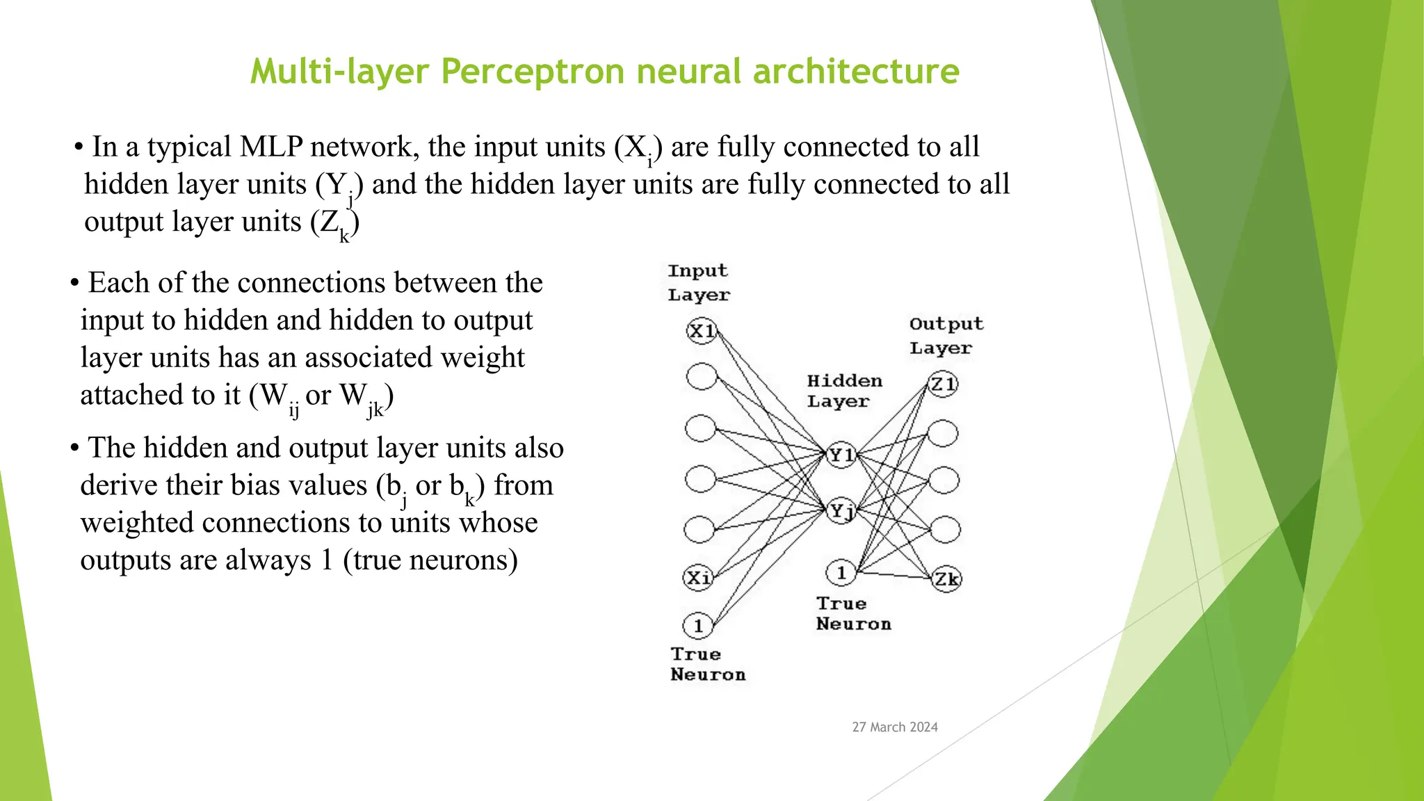
27 March 2024 Multi-layer Perceptron neural architecture • In a typical MLP network, the input units (Xi ) are fully connected to all hidden layer units (Yj ) and the hidden layer units are fully connected to all output layer units (Zk ) • Each of the connections between the input to hidden and hidden to output layer units has an associated weight attached to it (Wij or Wjk ) • The hidden and output layer units also derive their bias values (bj or bk ) from weighted connections to units whose outputs are always 1 (true neurons)

27 March 2024 MLP training algorithm A Multi-Layer Perceptron (MLP) neural network trained using the Backpropagation learning algorithm is one of the most powerful forms of supervised neural network system. The training of such a network involves three stages: • feedforward of the input training pattern, • calculation and backpropagation of the associated error • adjustment of the weights This procedure is repeated for each pattern over several complete passes (epochs) through the training set. After training, application of the net only involves the computations of the feedforward phase.

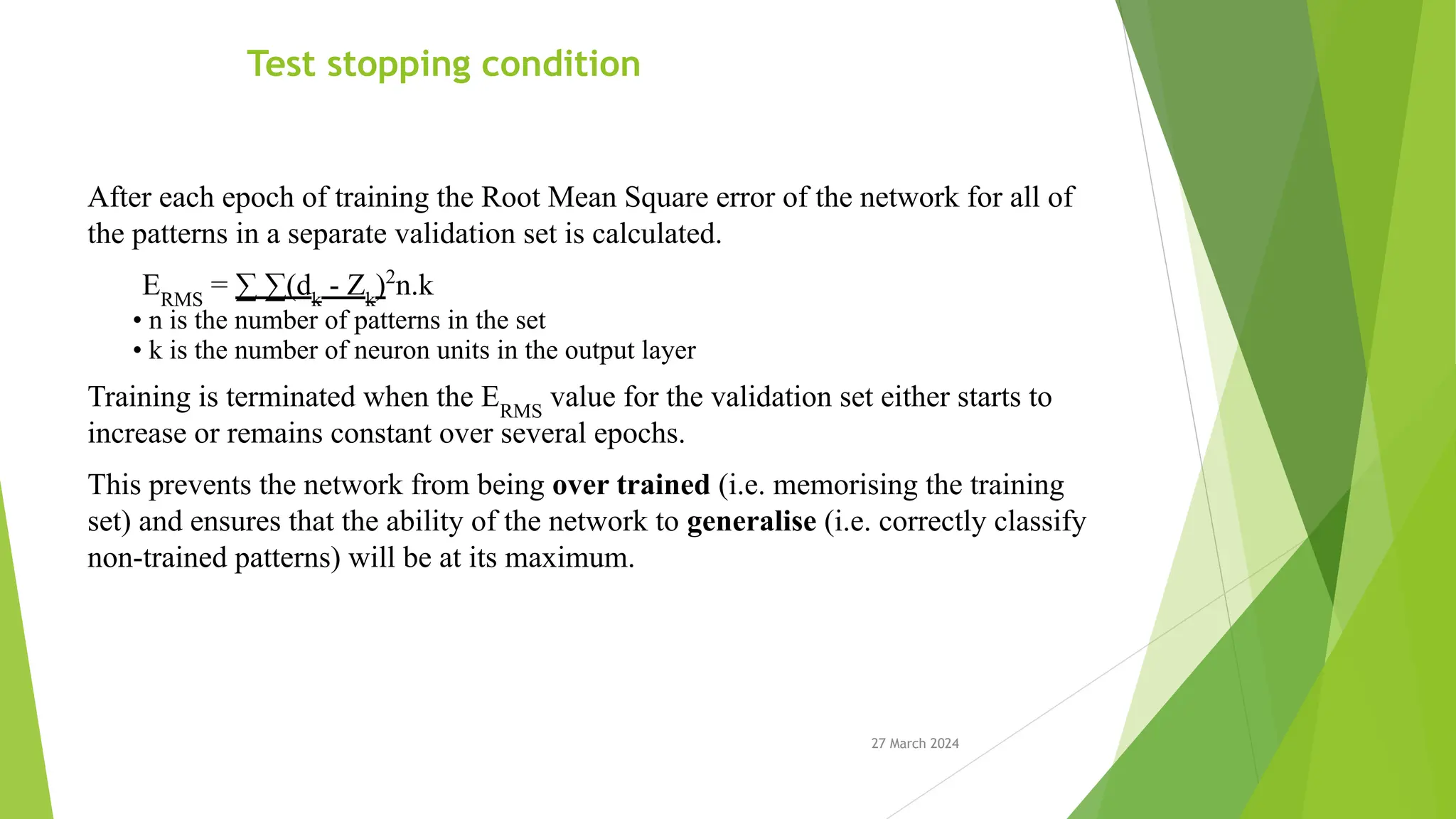
27 March 2024 Backpropagation Learning Algorithm Feed Forward phase: • Xi = input[i] • Yj = f( bj + ∑Xi Wij ) • Zk = f( bk + ∑Yj Wjk ) Backpropagation of errors: • δk = Zk [1 - Zk ](dk - Zk ) • δj = Yj [1 - Yj ] ∑ δk Wjk Weight updating: • Wjk (t+1) = Wjk (t) + ηδk Yj + α[Wjk (t) - Wjk (t - 1)] • bk (t+1) = bk (t) + ηδk Ytn + α[bk (t) - bk (t - 1)] • Wij (t+1) = Wij (t) + ηδj Xi + α[Wij (t) - Wij (t - 1)] • bj (t+1) = bj (t) + ηδj Xtn + α[bj (t) - bj (t - 1)]

27 March 2024 Test stopping condition After each epoch of training the Root Mean Square error of the network for all of the patterns in a separate validation set is calculated. ERMS = ∑ ∑(dk - Zk )2 n.k • n is the number of patterns in the set • k is the number of neuron units in the output layer Training is terminated when the ERMS value for the validation set either starts to increase or remains constant over several epochs. This prevents the network from being over trained (i.e. memorising the training set) and ensures that the ability of the network to generalise (i.e. correctly classify non-trained patterns) will be at its maximum.

27 March 2024 Factors affecting network performance Number of hidden nodes: • Too many and the network may memorise training set • Too few and the network may not learn the training set Initial weight set: • some starting weight sets may lead to a local minimum • other starting weight sets avoid the local minimum. Training set: • must be statistically relevant • patterns should be presented in random order Date representation: • Low level - very large training set might be required • High level – human expertise required

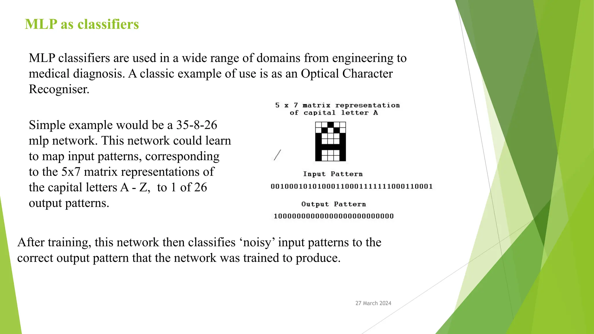
27 March 2024 MLP as classifiers MLP classifiers are used in a wide range of domains from engineering to medical diagnosis. A classic example of use is as an Optical Character Recogniser. Simple example would be a 35-8-26 mlp network. This network could learn to map input patterns, corresponding to the 5x7 matrix representations of the capital letters A - Z, to 1 of 26 output patterns. After training, this network then classifies ‘noisy’ input patterns to the correct output pattern that the network was trained to produce.

Adaline neural network • The Adaptive Linear Neuron, abbreviated as Adaline, is one of the fundamental artificial neural networks (ANNs) used in machine learning and artificial intelligence. It was introduced by Bernard Widrow and his graduate student Ted Hoff in 1960. • Adaline is closely related to the perceptron, another early neural network model. In fact, Adaline can be seen as a single-layer neural network, similar to the perceptron, with a linear activation function. However, unlike the perceptron, Adaline's output is not binary; instead, it outputs a continuous value. This makes it suitable for regression tasks rather than just classification.

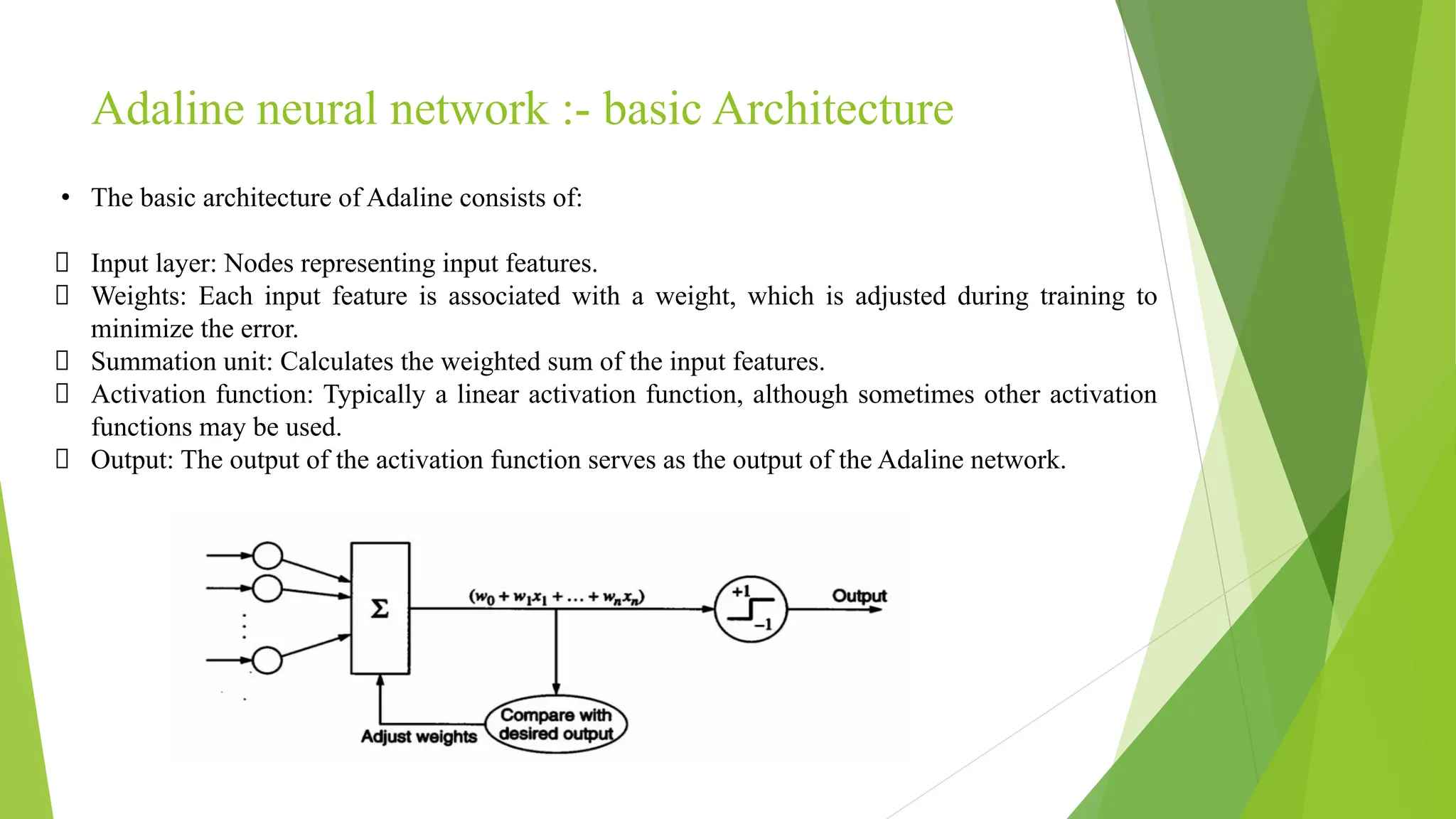
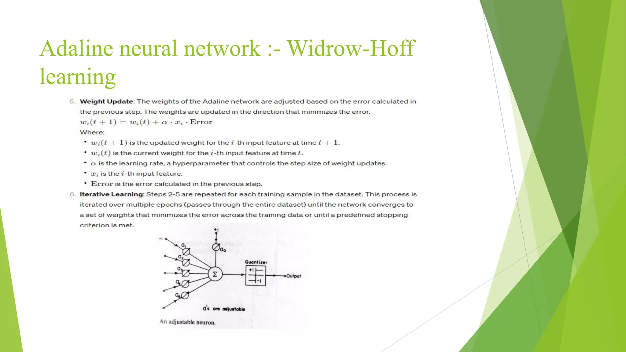
Adaline neural network :- basic Architecture • The basic architecture of Adaline consists of: Input layer: Nodes representing input features. Weights: Each input feature is associated with a weight, which is adjusted during training to minimize the error. Summation unit: Calculates the weighted sum of the input features. Activation function: Typically a linear activation function, although sometimes other activation functions may be used. Output: The output of the activation function serves as the output of the Adaline network.

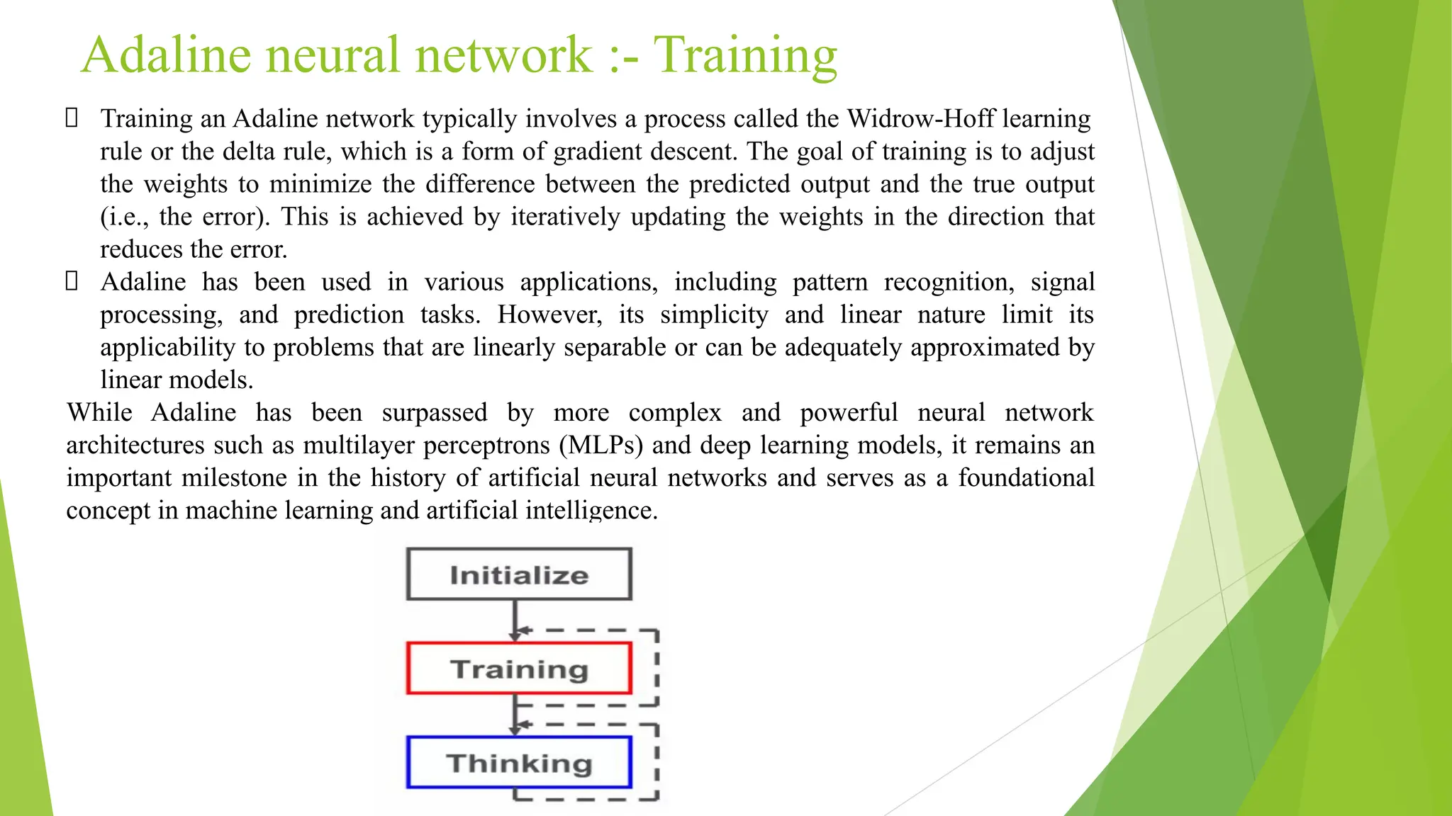
Adaline neural network :- Training Training an Adaline network typically involves a process called the Widrow-Hoff learning rule or the delta rule, which is a form of gradient descent. The goal of training is to adjust the weights to minimize the difference between the predicted output and the true output (i.e., the error). This is achieved by iteratively updating the weights in the direction that reduces the error. Adaline has been used in various applications, including pattern recognition, signal processing, and prediction tasks. However, its simplicity and linear nature limit its applicability to problems that are linearly separable or can be adequately approximated by linear models. While Adaline has been surpassed by more complex and powerful neural network architectures such as multilayer perceptrons (MLPs) and deep learning models, it remains an important milestone in the history of artificial neural networks and serves as a foundational concept in machine learning and artificial intelligence.

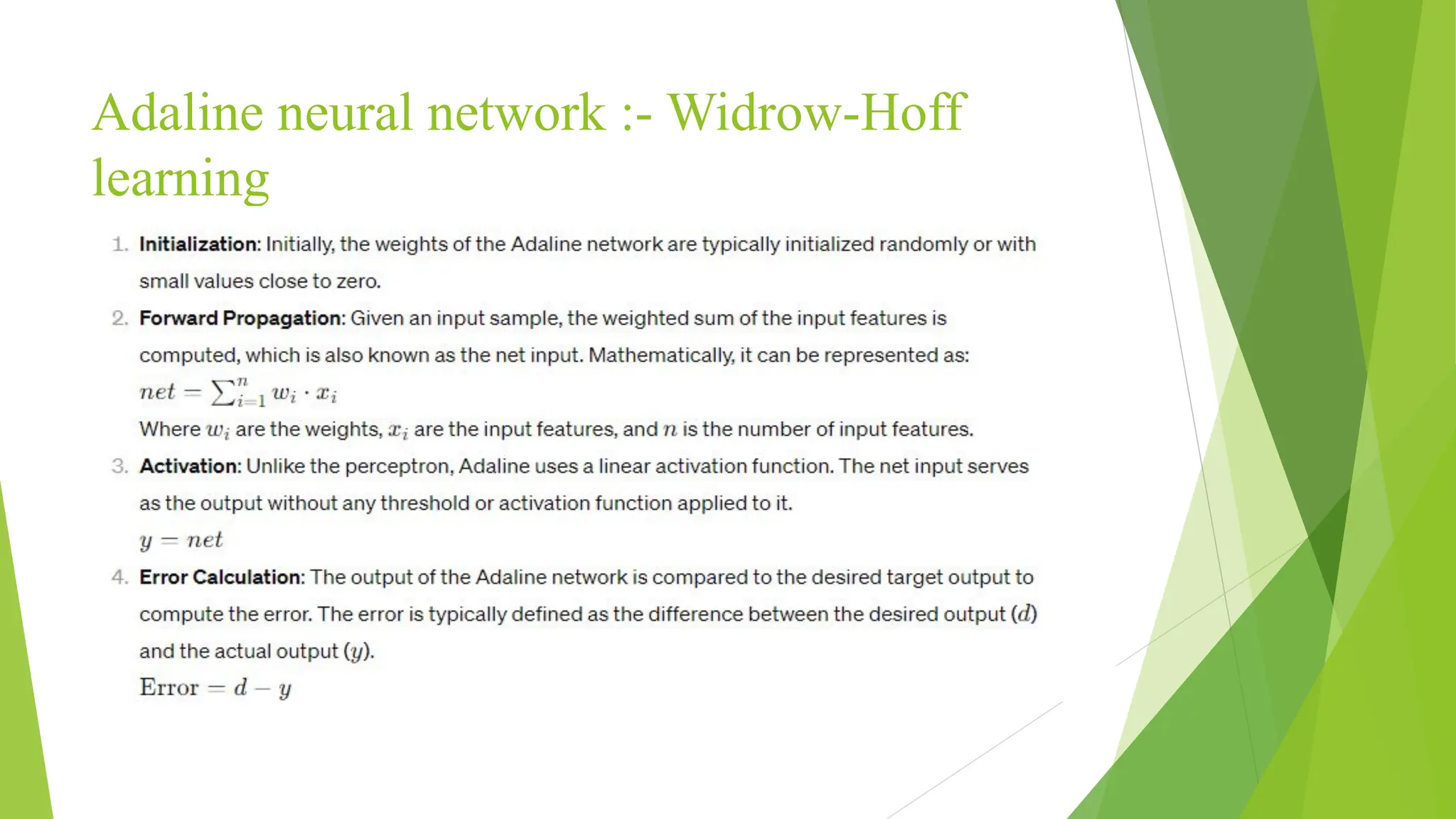
Adaline neural network :- Widrow-Hoff learning The Widrow-Hoff learning rule, also known as the delta rule or the LMS (Least Mean Squares) algorithm, is the primary learning algorithm used to train the Adaline (Adaptive Linear Neuron) neural network. The goal of the learning process is to adjust the weights of the network in such a way that the output closely matches the desired target output for a given input. Here's an overview of how the Widrow-Hoff learning rule works with Adaline. 1. Initialization. 2. Forward Propagation. 3. Activation. 4. Error Calculation. 5. Weight Update. 6. Iterative learning.

Adaline neural network :- Widrow-Hoff learning

Backpropagation Algorithm:- introduction & Training Procedure Backpropagation is a fundamental algorithm used for training artificial neural networks, particularly multilayer perceptrons(MLPs) and deep neural networks (DNNs). It is a supervised learning algorithm that adjusts the weights of the network to minimize the difference between the predicted output and the actual target output. Here's an overview of how backpropagation works: 1.Forward Pass: • Input data is fed into the neural network, and computations are performed layer by layer to generate an output. • Each layer computes a weighted sum of its inputs, applies an activation function to the sum, and passes the result to the next layer. 2. Compute Error: • Once the output is generated, the error between the predicted output and the actual target output is computed using a loss function. • Common loss functions include mean squared error (MSE) for regression problems and categorical cross-entropy for classification problems.

Backpropagation Algorithm:- introduction & Training Procedure 3.Backward Pass (Backpropagation): • Backpropagation involves propagating the error backward through the network to update the weights. • Starting from the output layer, the gradient of the loss function with respect to the weights and biases of each layer is computed. This is done using the chain rule of calculus, which allows for the computation of gradients layer by layer. 4. Weight Update: • Once the gradients are computed, the weights and biases of each layer are updated in the opposite direction of the gradient to minimize the loss function. • The update rule typically involves subtracting a fraction of the gradient from the current weights, scaled by a learning rate hyper parameter. • The learning rate controls the step size of the weight updates and is crucial for the convergence and stability of the training process.

Backpropagation Algorithm:- introduction & Training Procedure 5.Iterative Training: Steps 1-4 are repeated iteratively for multiple epochs (passes through the entire dataset) until the network converges or until a stopping criterion is met. During each epoch, the network sees the entire dataset in batches or as individual samples, depending on the training strategy (e.g., mini-batch gradient descent, stochastic gradient descent). Backpropagation enables neural networks to learn complex patterns and relationships in data by iteratively adjusting their weights to minimize prediction errors. It has been instrumental in the success of deep learning, allowing for the training of neural networks with many layers, which are capable of solving a wide range of tasks across various domains, including image recognition, natural language processing, and speech recognition.

Tuning the Network Size Tuning the network size in an artificial neural network (ANN) refers to adjusting the architecture of the network, including the number of layers and the number of neurons in each layer, to achieve optimal performance for a specific task. This process involves finding the right balance between model complexity and generalization ability. key considerations and steps involved in tuning the network size:- 1.Start with a Baseline Model: Begin by constructing a baseline ANN architecture with a reasonable number of layers and neurons. This initial model serves as a reference point for comparison when evaluating the performance of subsequent models. 2.Understand the Problem Complexity: Consider the complexity of the problem you are trying to solve. Complex tasks, such as image recognition or natural language processing, may require larger and more complex networks to capture intricate patterns and relationships in the data. 3Avoid Overfitting: Overfitting occurs when the model learns to memorize the training data instead of generalizing to unseen data. Increasing the network size can exacerbate overfitting, especially when dealing with limited training data. Regularization techniques, such as dropout and weight decay, can help mitigate overfitting by introducing constraints on the model parameters.

Tuning the Network Size 4.Evaluate Performance: Train the baseline model and evaluate its performance on a validation dataset. Common metrics for evaluation include accuracy, precision, recall, F1-score, and mean squared error, depending on the nature of the task (classification or regression). 5.Experiment with Network Size: Systematically vary the network size by adjusting the number of layers and neurons in each layer. Explore different configurations, including shallow vs. deep networks, wide vs. narrow networks, and the number of hidden units in each layer. 6.Monitor Training and Validation Performance: During training, monitor both training and validation performance to detect signs of overfitting or underfitting. Overfitting typically manifests as a large gap between training and validation performance, whereas underfitting indicates that the model is too simple to capture the underlying patterns in the data. 7.Use Cross-Validation: Employ techniques like k-fold cross-validation to assess the generalization performance of different network sizes more reliably. Cross-validation involves partitioning the dataset into multiple subsets, training the model on different subsets, and evaluating its performance on the remaining subset.

Tuning the Network Size 8.Select the Optimal Network Size: Choose the network size that achieves the best balance between performance and generalization ability based on the evaluation metrics. It's essential to strike a balance between model complexity and simplicity, ensuring that the selected architecture can generalize well to unseen data. 9.Fine-Tuning: Once the optimal network size is determined, fine-tune other hyper parameters, such as learning rate, batch size, and activation functions, to further optimize the model's performance. 10.Test the Final Model: Assess the final model's performance on a separate test dataset that was not used during training or validation. This step provides an unbiased estimate of the model's generalization ability in real-world scenarios. By systematically tune the size of network we can develop an optimal ANN.

Artificial Neural Network for machine learning

In this document

More Related Content

What's hot

Similar to Artificial Neural Network for machine learning

Recently uploaded

Artificial Neural Network for machine learning