Download as PDF, PPTX


![LOSS FUNCTION • A loss function (cost function) tells us how good our current model is, or how far away our model to the real answer. 𝐿(𝑤) = 1 𝑁 𝑖 𝑁 𝑙𝑜𝑠𝑠 (𝑓(𝑥 𝑖 ; 𝑤), 𝑦 𝑖 ) • Hinge loss • Softmax loss • Mean Squared Error (L2 loss) Regression 𝐿(𝑤) = 1 𝑁 ∑𝑖 𝑁 𝑓 𝑥 𝑖 ; 𝑤 − 𝑦 𝑖 2 • Cross entropy Loss Classification 𝐿 𝑤 = 1 𝑁 ∑𝑖 𝑁 [ 𝑦 𝑖 𝑙𝑜𝑔 𝑓 𝑥 𝑖 ; 𝑤 + 1 − 𝑦 𝑖 log 1 − 𝑓 𝑥 𝑖 ; 𝑤 ] • … N = # examples predicted actual](https://image.slidesharecdn.com/2018-03-17meetup-180319032650/75/Deep-Feed-Forward-Neural-Networks-and-Regularization-15-2048.jpg)

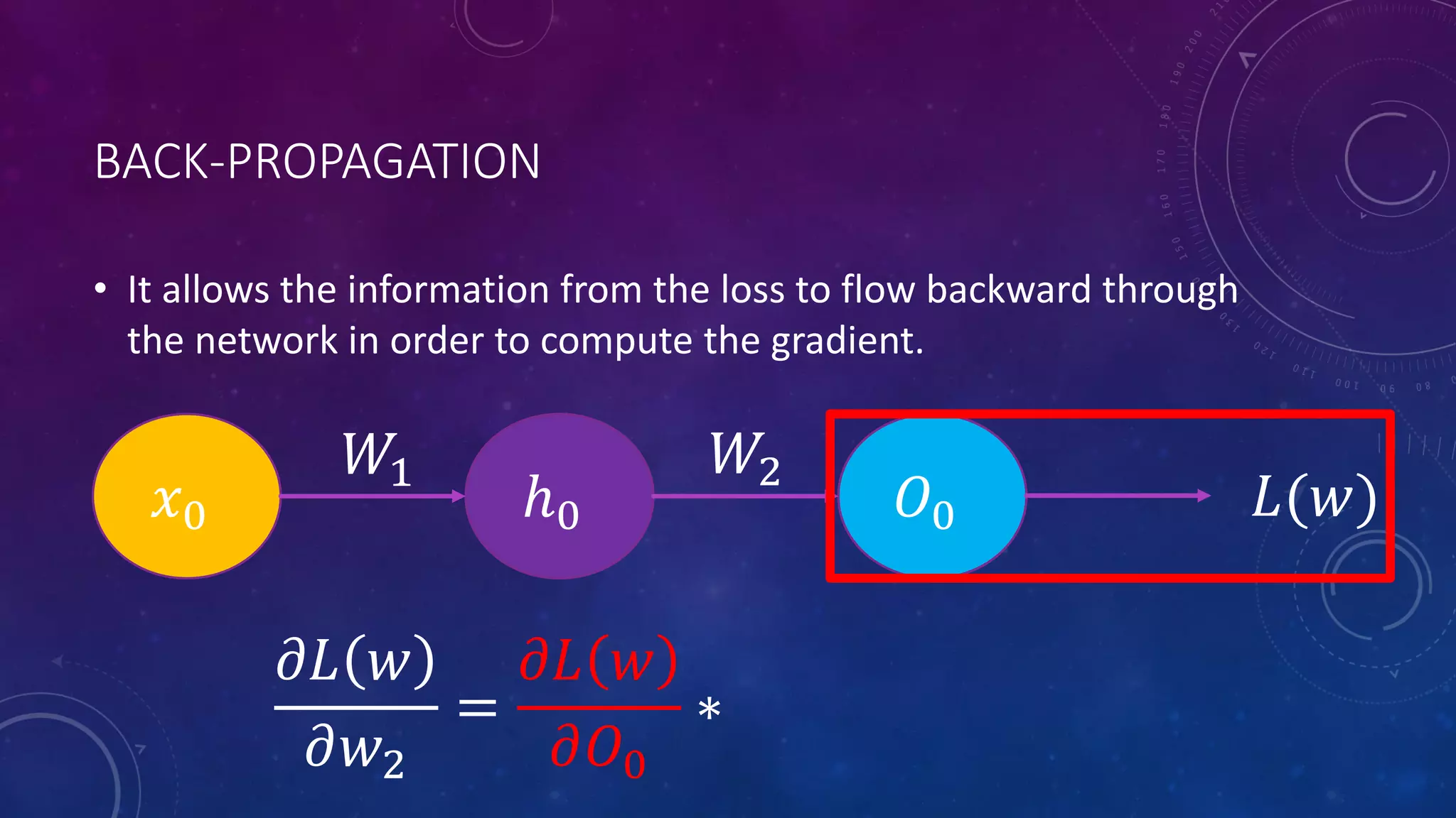
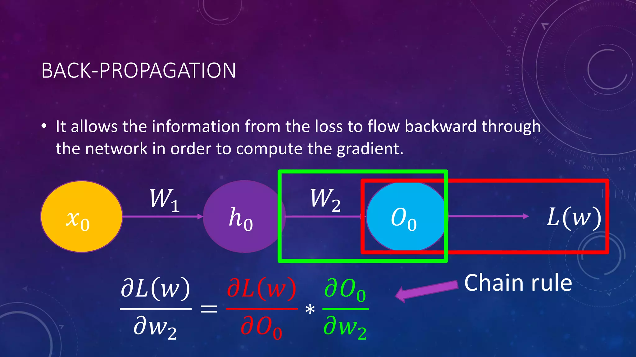
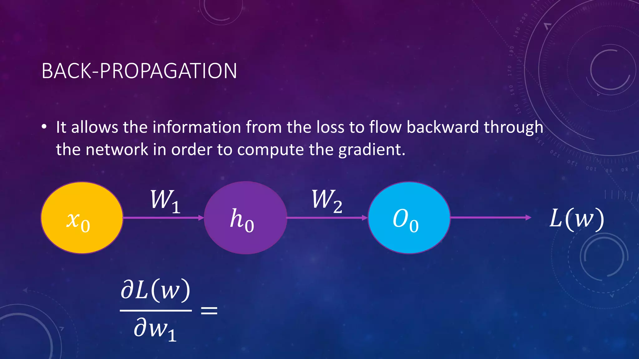
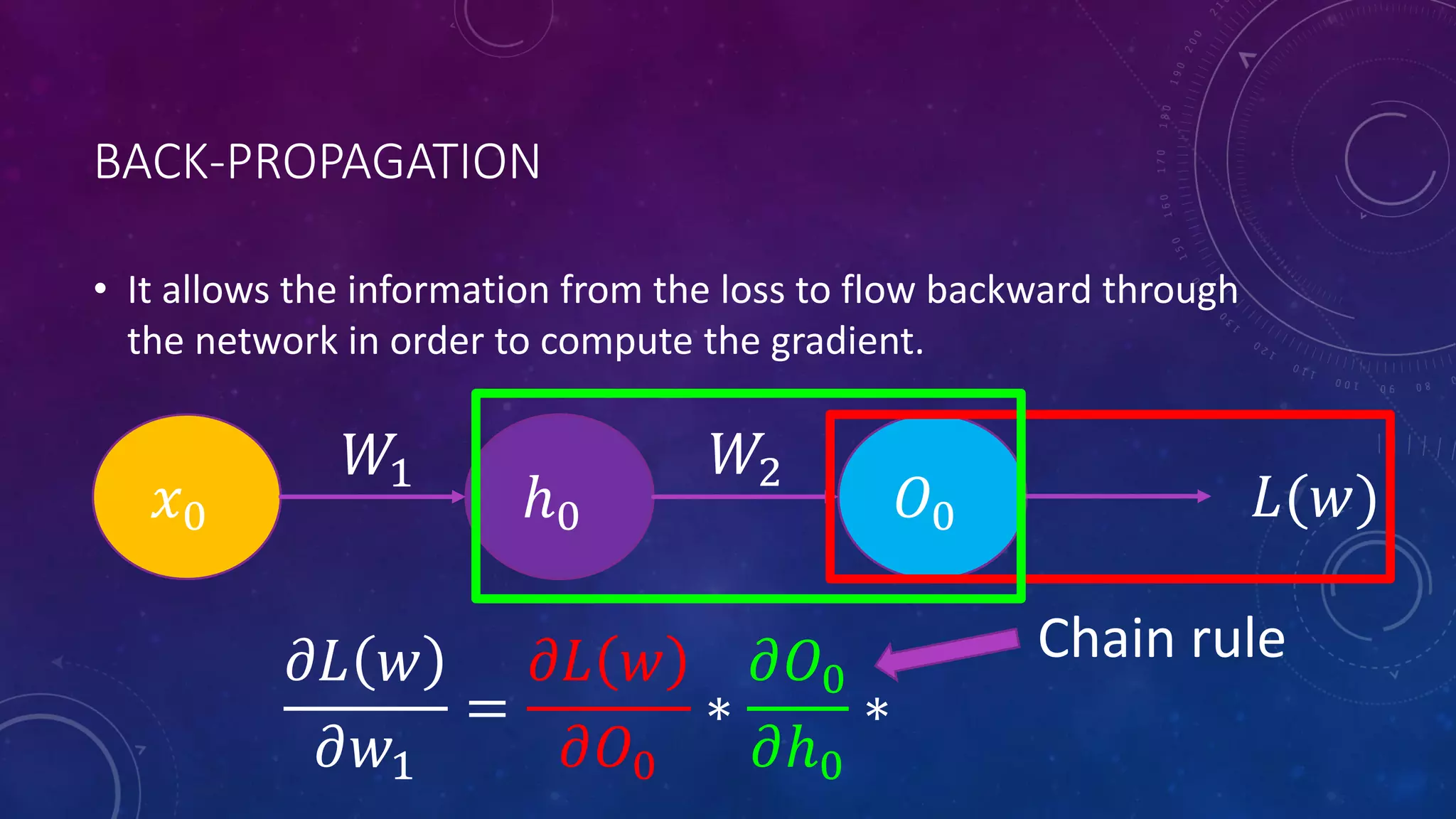
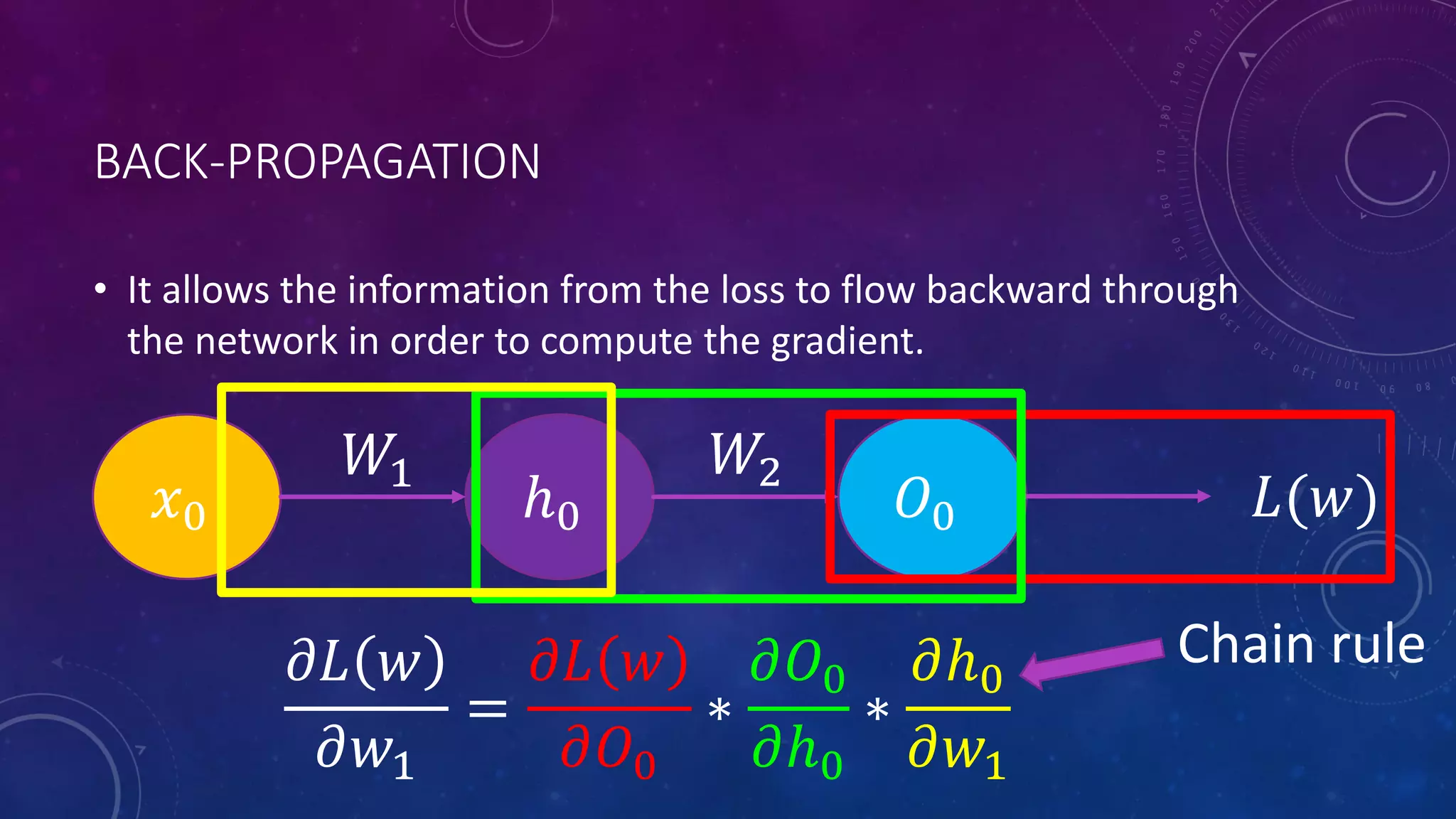
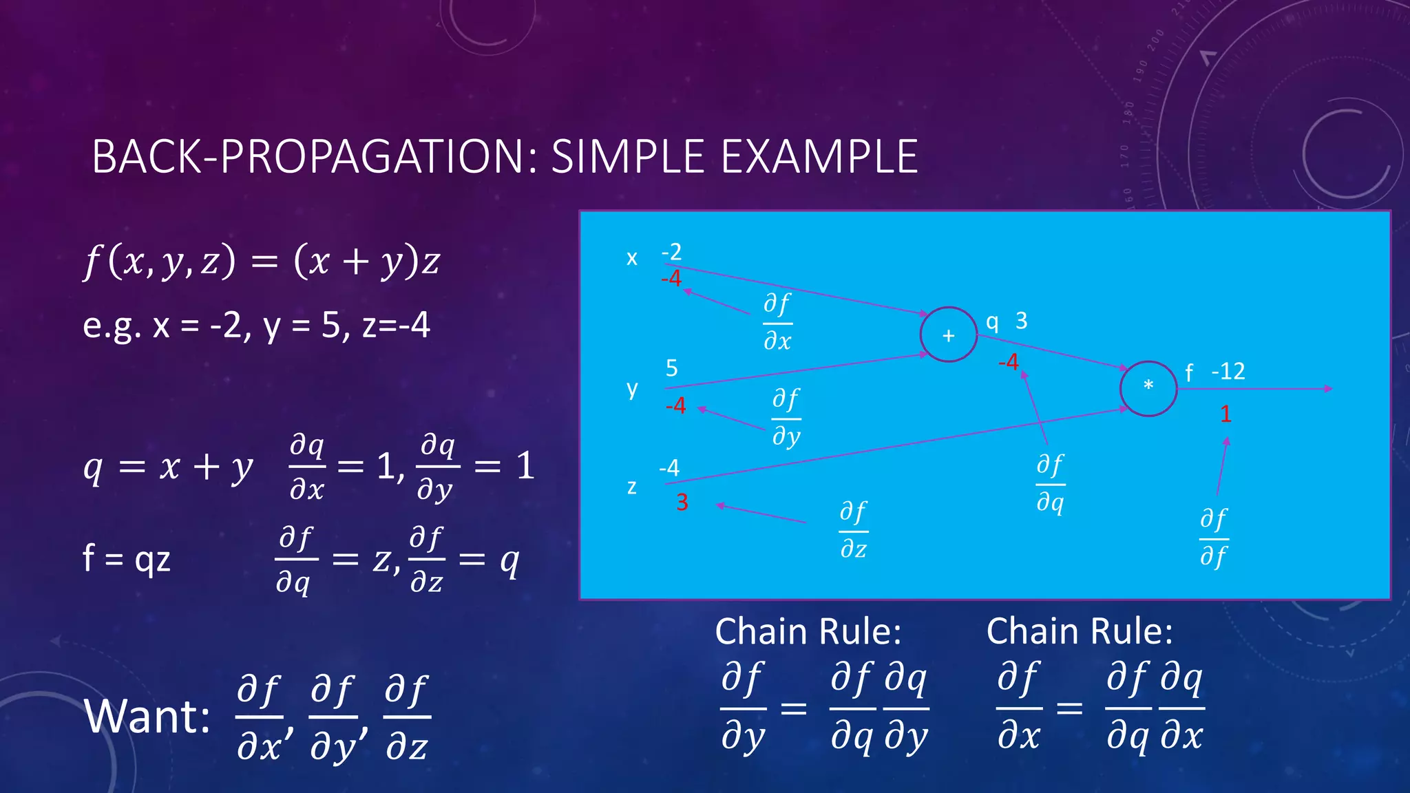


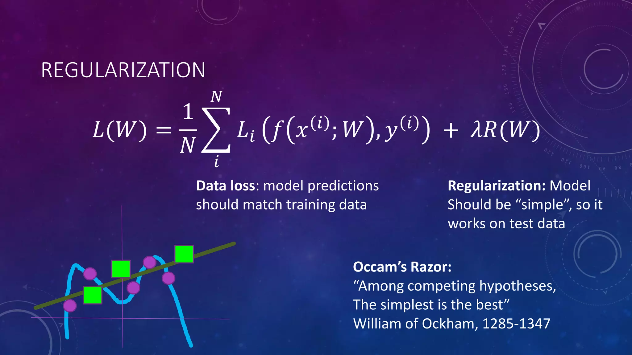

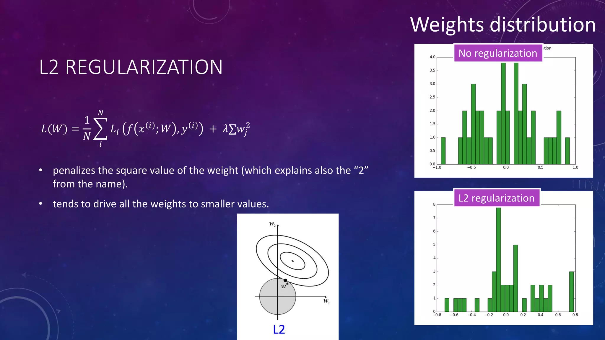
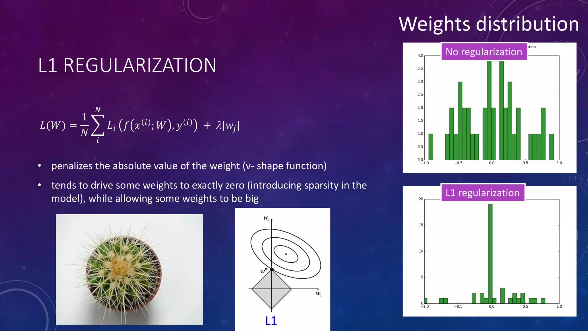
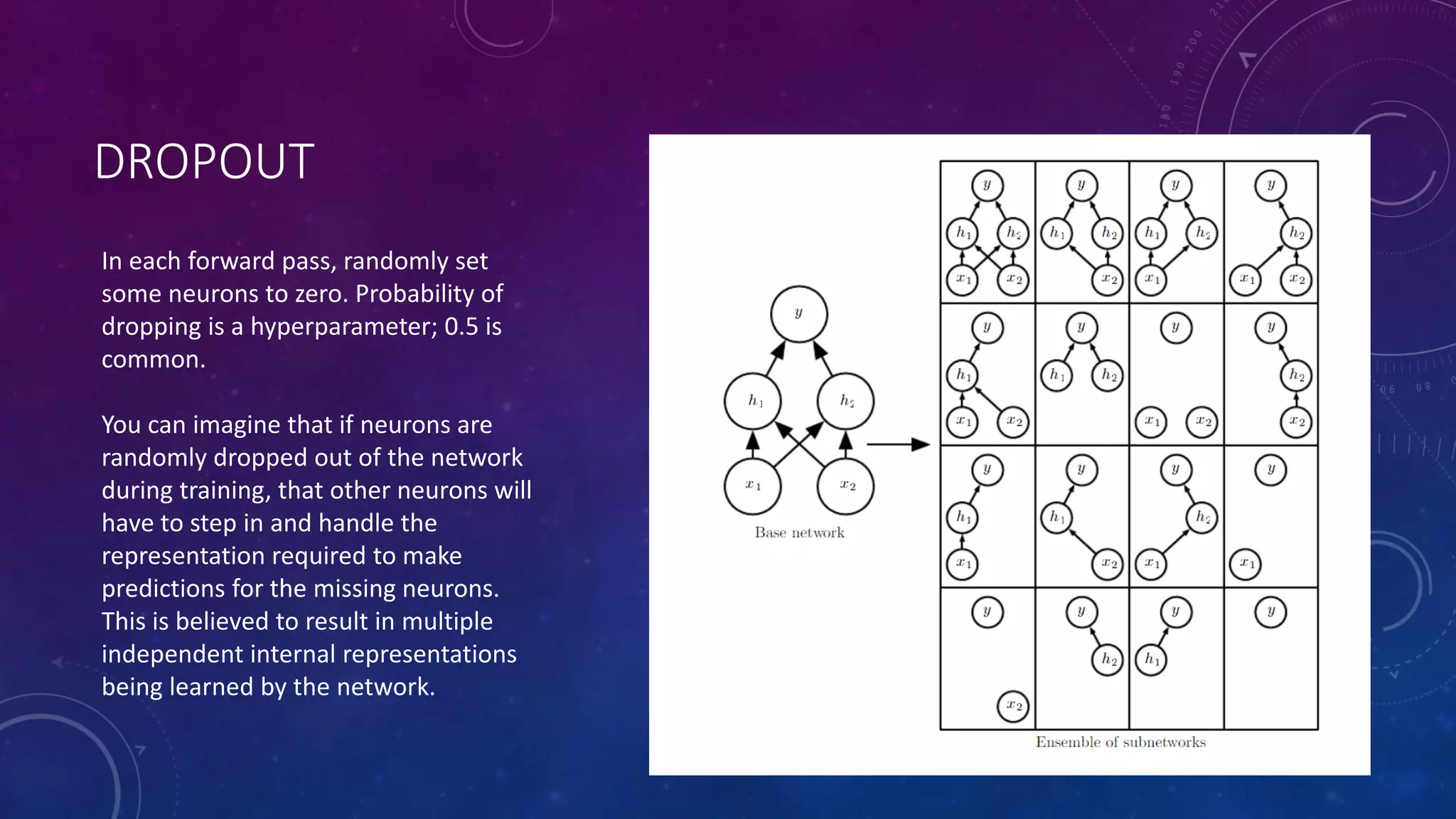
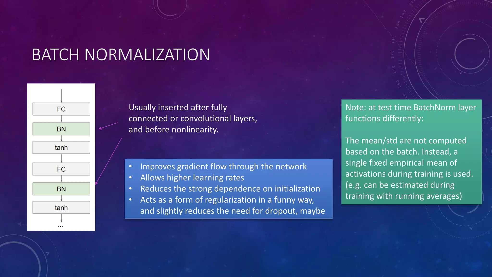
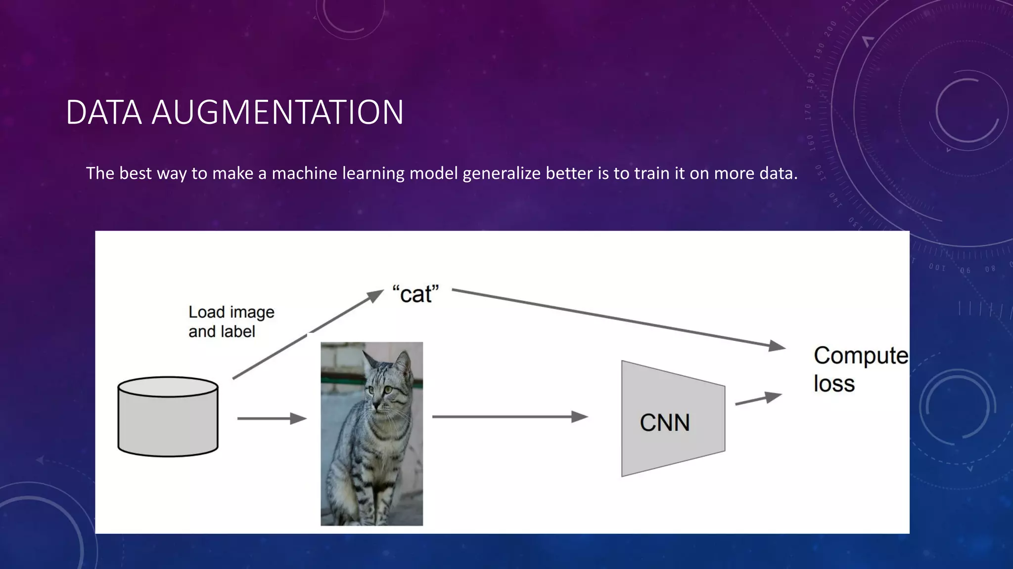
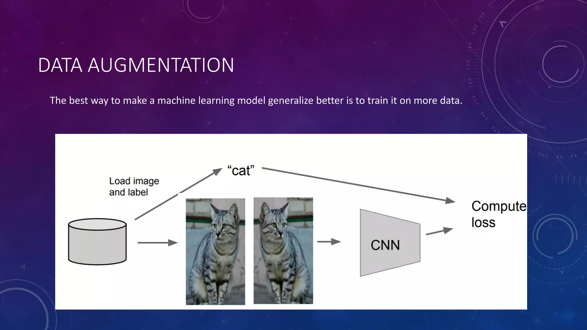
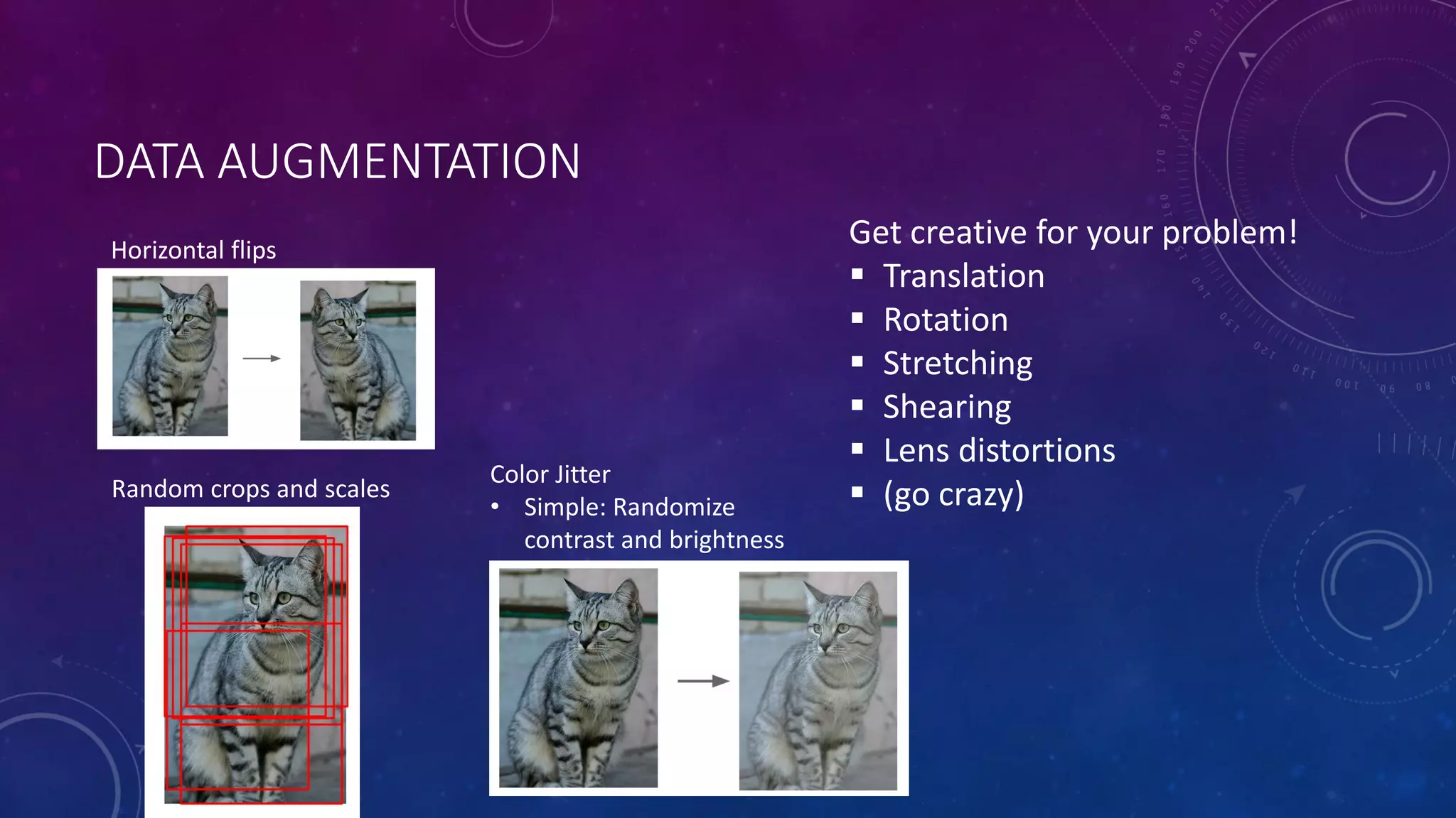


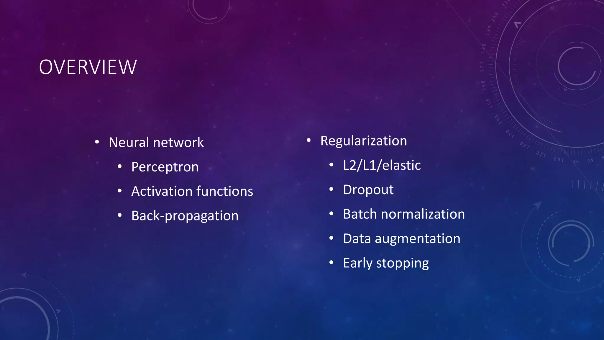
Deep feedforward networks use regularization techniques like L2/L1 regularization, dropout, batch normalization, and early stopping to reduce overfitting. They employ techniques like data augmentation to increase the size and variability of training datasets. Backpropagation allows information about the loss to flow backward through the network to efficiently compute gradients and update weights with gradient descent.