Download to read offline
![International Journal of Research in Advanced Technology - IJORAT Vol. 1, Issue 3, DECEMBER 2015 All Rights Reserved © 2015 IJORAT Page 1 An Adaptive Differential Evolution Algorithm for Reactive Power Dispatch Arun.G1 , Chandrasekar.T2 PG Scholar, M.E (PSE), Velammal College of Engineering and Technology, Madurai, India 1 Assistant Professor, M.E ,VelammalCollege of Engineering and Technology, Madurai, India 2 Abstract: Reactive power or VAR management is one of the most crucial tasks required for proper operation and control of a power system. Reactive power management is carried out to reduce losses in a power system, by adjusting the reactive power control variables such as generator voltages transformer tap-setting and other sources of reactive power such as capacitor banks or FACTS devices. VAR management provides better system security improved power transfer capability and overall system operation. VAR management is a complex combinatorial optimization problem involving non-linear functions having multiple local minima and non-linear and discontinuous constraints. In this paper, the VAR management problem is formulated as a non- linear constrained optimization problem with equality and inequality constraints for minimization of real power loss. The problem is solved using Differential evolution (DE), which is a population based search algorithm. For avoiding the time and the effort in tuning the parameters of DE algorithm, an Adaptive DE algorithm with time varying chaotic mutation and crossover is proposed for solving the optimization problem. Effectiveness of the proposed an Adaptive DE algorithm based approach has been demonstrated on the IEEE 57-bus and IEEE 118-bus system are found to be superior to classical DE and its variants Self- adaptive Differential Evolution (SaDE) in terms of convergence behavior and solution quality. Keywords:Adaptive differential Evolution algorithm, Real power loss minimization, VAR management,Voltage deviation. I. INTRODUCTION The main objective of reactive power (VAR) management in a power system is to identify the reactive power control variables settings such as generator voltages, transformer tap settings and other sources of reactive power such as capacitor banks or FACTS devices to reduce losses, system security, power transfer capability and overall system operation. Reactive power management is a sub problem of optimal power flow (OPF) calculation. OPF is an on-linear programming (NLP) problem that is solved find out the optimal control parameters/circumstance to minimize a desired objective function, subject to certain system constraints. It was first introduced by Carpentier [1,2] in 1960s.Reactive power management provides the power system operator a set of control variables to minimize transmission losses and to preserve bus voltage within permissible limits by rescheduling the power flows. In recent years, the issue of reactive power management for various objectives like voltage control and power loss reduction has received much attention. The main objective of VAR management is to improve the voltage profile and minimize real power losses through redistribution of reactive power in the system[3-5]. Through, the conventional optimization techniques like Gradient method, non-linear programming and interior point method can be applied to solve VAR management problem [6-10], but these techniques have several drawbacks, such as insecure convergence properties and excessive numerical iterations: resulting in huge computations and large execution time. Also, these methods are highly complex optimization techniques and insufficient for large-scale system applications [10]. Due to non- differential, non-linear, multi- modal and non- convex nature of the VAR management problem, most of these conventional techniques converge to local optimum[10]. With the advent of Evolutionary computing (EC) techniques like Genetic Algorithm (GA), Evolutionary programming (EP), Differential Evolution (DE) algorithm and Particle swarm optimization (PSO), these techniques have been applied for reactive power dispatch problem [11- 21]. These nature inspired stochastic search based methods are increasingly being proposed for solving power system optimization problems in recent years. The random parallel search capability and non-dependency on nature of the optimization problem has contributed to their popularity for handling various complexoptimization problems. The ease of formulating the equality and inequality constraints and stable convergence behavior also add to their merits. In recent years, Some evolutionary computing based algorithms, their advanced versions and hybrid EC algorithms have been developed and proposed for various optimization problems in power system[22, 23]. The advanced versions and hybrid EC algorithms are claimed to provide better solution for some functions and the problem under considerations, but there is no algorithm available which out performs other algorithms for all the optimization problems. The reason is that, these methods do not converge to the global best solution in every trial run but are able to produce a feasible near solution quit fast and are highly depend on parameter tuning. DE is the simple population based search algorithm, which is highly efficient in handling constrained optimization problems and is supposed to be an improved version of Genetic algorithm. This algorithm can be applied for optimization of a non-smooth, discontinuous and multi- modal function. Differential Evolution algorithm can find near optimal solution regardless the initial parameters, its](https://image.slidesharecdn.com/vol1issue3p001-160121144600/75/An-Adaptive-Differential-Evolution-Algorithm-for-Reactive-Power-Dispatch-1-2048.jpg)
![International Journal of Research in Advanced Technology - IJORAT Vol. 1, Issue 3, DECEMBER 2015 All Rights Reserved © 2015 IJORAT Page 2 convergence is fast and it requires a few numbers of parameters. In addition to this, its coding is simple and it can handle integer and discrete optimization [24, 25]. The performance of the Differential Evolution algorithm was compared with various heuristic techniques. It has been observed that DE algorithm is significantly better than that of other heuristic methods like GA, Particle swarm optimization and Evolutionary Algorithm.DE algorithm is found to be robust and able to provide the same results consistently over several trials [26, 27]. In addition to this, DE algorithm has been used to solve high dimensional function optimization [28]. It is found that, it has superior functioning on o set of widely used bench mark functions. Thus, DE algorithm seems to be a promising approach for various engineering optimization problems including reactive power management [29-32]. Differential evolution algorithm has been applied for single objective VAR management problem [18,19].and the results obtained are found to be better than those already reported earlier by using other such techniques. In this paper An Adaptive DE with time varying chaotic mutation and crossover has been proposed for solving the single objective VAR management problem. The problem has been formulated as a non-linear constrained single objective optimization problem, where the real power loss and the bus voltage deviations are to be optimized (minimized) simultaneously. Effectiveness of the proposed an Adaptive DE based approach to solve single objective VAR management problem has been demonstrated and compared on the standard IEEE 57-bus and IEEE 118-bus system[6]. II. PROBLEM FORMULATION AThe optimal VAR management problem is to optimize the steady state performance of a power system in terms of one or more objective functions while satisfying several equality and inequality constraints. The VAR management problemcan be formulated as follows [4]. 2.1 objective function 1. Minimization of real power loss (PL) This objective is to minimize the real power loss in transmission lines of a power system by managing reactive power and is expressed as F1=Ploss=∑nl K=1gk[Vi 2 +Vj 2 -2ViVj(δi-δj)] (1) 2.2 Problem constraints (1) Equality constraints The equality constraints represent typical load flow equations as follows PGi-PDi-Vi∑j≠1 Vj(Gijcosθij+ Bijsin θij)= 0 (2) Where θij=(δi– δj) QGi-QDi-Vi∑j≠1 Vj(Gijsin θij- Bijcosθij)= 0 (3) Whereθij=(δi– δj) For i=1,2,3…..NB (2) Inequality constraints The inequality constraints represent the system operating constraints as follows, a. Generation constraints: Generator voltages VG and reactive power outputs QG are restricted by their lower and upper limits as follows: Vi-min ≤Vi ≤ Vi-max (4) QGi-min≤QGi≤QGi-maxiЄ{Npv,N0}(5) b. Transformer constraints: Transformer tap T settings are bounded as follows: Ti-min≤ Ti ≤ Ti-max i Є NT(6) c. Switchable VAR sources constraints: Switchable VAR compensations Qc are restricted by their limits as follows: QCi-min≤QCi≤QCi-maxiЄNC(7) d. Security constraints: These include the constraints of voltages at load buses VL and transmission line loadings SL as follows:as follows: Vli-min ≤ Vli≤Vli-max i = 1,2,……NLB (8) Sli-min≤ Sli-max i = 1,2,……NLB (9) Aggregating the objectives and constraints, the problem can be mathematically formulated as a non-linear constrained multi-objective optimization problemas follows: Minimize [PL(x,u)] (10) Subject to : Equality constraint g(x,u)=0 (11) And Inequality constraint h(x,u) < 0 (12) Here x can be expressed as XT =[VL1…….VNLB,QG1…....QGNG,SL1……Sint] (13) While u can be expressed as UT =[VG1…….VGNG,T1…….TNT,Qc1……..QCNC] (14) I. Adaptive Differential Evolution algorithm has been applied for this multi-objective VAR management problem, which is a combinatorial optimization problem having multi-extremism and non-linear property. In this paper, the reactive power management. III. CLASSICAL DIFFERENTIAL EVOLUTIONARY ALGORITHM A Differential Evolution (DE) is a population based algorithmthat employs crossover, mutation (differential) and selection operators. In differential Evolution, all the solutions have the same probability of being selected as parents. DE employs a greedy selection process that is the best new solution and its parent win the competition](https://image.slidesharecdn.com/vol1issue3p001-160121144600/75/An-Adaptive-Differential-Evolution-Algorithm-for-Reactive-Power-Dispatch-2-2048.jpg)
![International Journal of Research in Advanced Technology - IJORAT Vol. 1, Issue 3, DECEMBER 2015 All Rights Reserved © 2015 IJORAT Page 3 providing significant advantage of converging performance over Genetic algorithms, Differential Evolution [18] algorithm works through a simple cycle of the stages as follows 3.1 Initialization At the beginning of DE algorithm implementation, i.e t=0 the problem independent variables are initialized somewhere in their feasible numerical range. Therefore, if the jth variable has its lower and upper bounds as xi andxj respectively, then the jth component of the ith population member may be initialized as: Xij(0)=Xj 1 +rand(0,1)*(Xj u –Xj l ) (15) Where rand(0,1) is a uniformly distributed random numbers between 0and 1. 3.2 Mutation In each generation, a donor vector V(t) is created in order to change the population member vector Xi(t). Generally, the method of creating this donor vector is different in various DE schemes. However, in this paper, DE/rand /1 mutation Strategy is implemented. In this mutation strategy, creation of the donor vector V(t)for the ith member Xi, three parameter vector Xr1,Xr2 and Xr2 are selected randomly from the current population not coinciding with the current member Xi. Next, a scalar number F scales the difference between any two of the three vectors and this scaled difference is added to the third one. Thus, the donor vector V(t) is obtained. The jth component of each vector can be expressed as: Vi,j(t+1)=Xr1,j(t)+F(Xr2,j(t)-Xr3,j(t)) (16) 3.3 Crossover To increase the diversity of the population, crossover operator is carried out in which the donor vector exchanges its components with those of the current member Xi(t). Two types of crossover schemes, namely exponential crossover and binomial crossover can be used by DE algorithm [24,25]. In this paper, binomial crossover scheme is used which is performed on all the D variables and can be expressed as: Ui,j(t)={Vi,j(t) if rand(0,1)< CR Xi,j(t) else (17) 3.4 Selection To keep the population size constant over subsequent generations, the selection process is applied to find out which one of the child and the parent will survive in the next generation, i.e at time t=t+1. Differential Evolution actually adopts the survival of the fittest principle in its selection process. The selection process can be expressed as Xi(t+1)={ Ui(t) iff (Ui(t)≤F(Xi(t)) Xi(t) iff(Xi(t)<F(Ui(t)) (18) Where F(.) is the function to be minimized. So ,if the child Ui(t) yields a better value of the fitness function, it replaces its parents in the next generation: otherwise, the parent Xi(t) is retained in the population. Thus the population either gets better in terms of the fitness function or remains fixed but never degenerates. Hence the population either gets better in terms of the fitness function or remains constant but never deteriorates. 3.4.1 Self-adaptive DE (SaDE) algorithm In Self adaptive DE (SaDE) algorithm, both strategies and their associated parameter are gradually Self-adapted by learning from their previous experiences in generating promising solutions. As a result, a more suitable generation strategy along with its parameter settings can be determined adaptively to match different search/evolution phases. In this algorithm, at each generation, a set of trial vector generation strategies together with their associated parameter values is separately assigned to different individual in current population according to the selection probabilities learned fromthe previous generations [32,34]. 3.4.3 An Adaptive DE algorithm Mutation rate F and crossover rate CR significantly affect the performance of the DE algorithm. The smaller the mutation rate F, longer time will be required for convergence of DE algorithm. While larger values of F allow exploration due to which the algorithm may not converge and skip good optimal solution. The value of F should be small to enough to enable the algorithm to explore tight valleys and large enough to allow global exploration in order to maintain population diversity. A higher CR creates more diversity and better exploration in the new population. In classical DE algorithm, both F and CR are fixed, so a lot of tuning parameters is required to achieve global best results. This problem can be solved by employing time - varying mutation and crossover rates. To improve the performance of classical DE, many hybrids of DE algorithm have been proposed that incorporates chaotic systems in various ways. The most common application of chaos theory in DE algorithm is for its parameter adaptation [36-38]. In addition to this, chaotic sequences have been utilized to initialize DE population diversity [36], to perform local search in the neighborhood of the selected individuals [40] etc. Chaotic sequences with the mutation factor have been integrated in DE algorithm to improve solution quality [38]. In [37], various chaotic sequences in evolutionary algorithms (EAs) were proposed in the place of the randomnumbers. In the present paper, the most commonly used chaotic sequence, known as logistics map has been applied to adapt the DE control parameters. The logistic equation is defined as follows: Y(t)=μ*Y(t-1)*[1-Y(t-1)] (19) Where t is the iteration count and μ is a control parameter 0≤ μ≤4. The behavior of the system represented by [26] significantly changes with the variation in μ. The value of μ controls the variation of the chaotic sequence. The DE variant with time varying F and CR is proposed in this paper. The variation of F chaotically, based on logistic map and time varying crossover rate CR, give rise to the following adaptive differential evolutionary algorithm: The mutation rate factor parameter F1is varied as per Eq.(16) where F1(0) lies between [0,1]. An index „t‟ is the current iteration and F1(t) is the new mutation factor based on the logistic map. F1(t)=μ*Y(t-1)*[1-F1(t-1)] (20) The control parameter μ decides whether mutation rate F1 oscillates between a limited sequences, varies chaotically or](https://image.slidesharecdn.com/vol1issue3p001-160121144600/75/An-Adaptive-Differential-Evolution-Algorithm-for-Reactive-Power-Dispatch-3-2048.jpg)
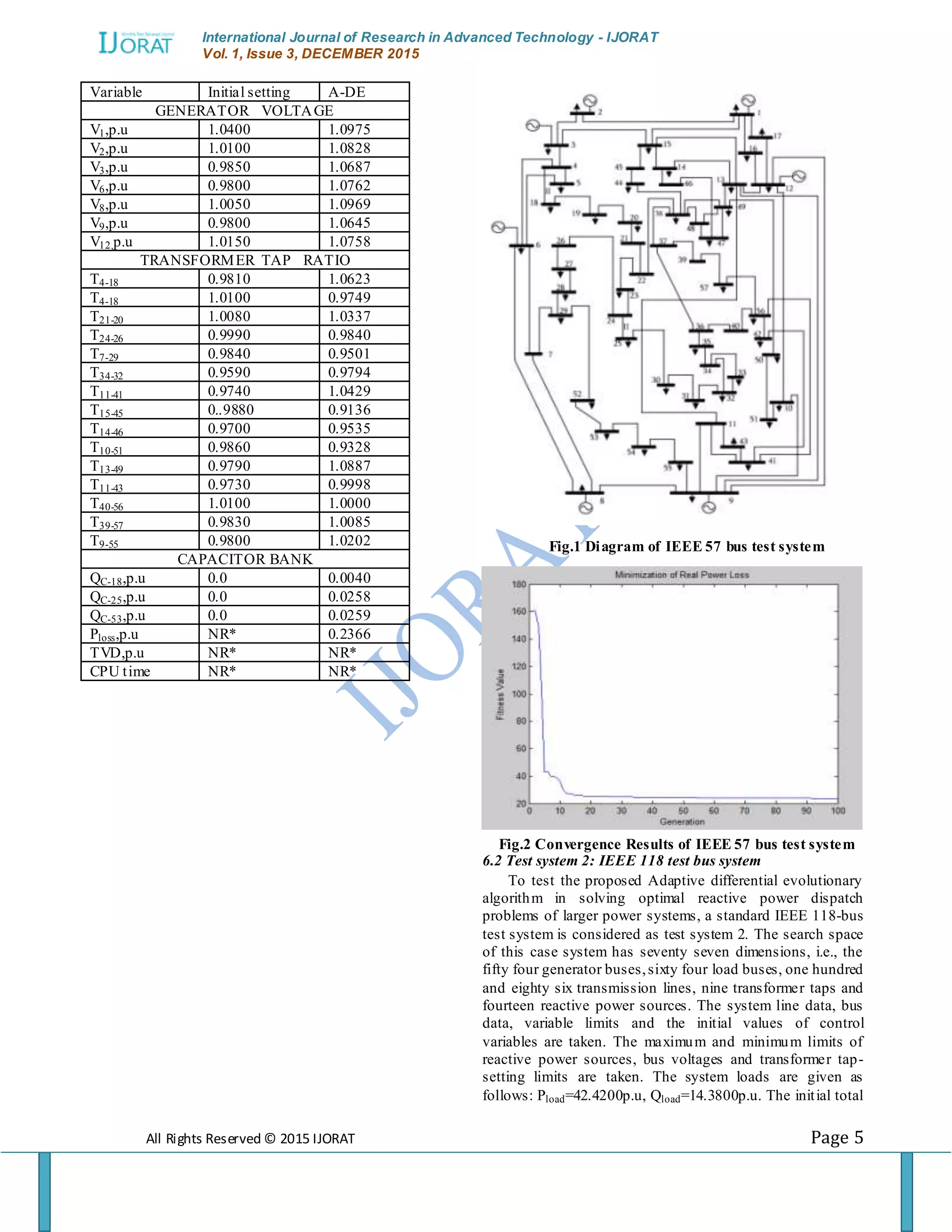
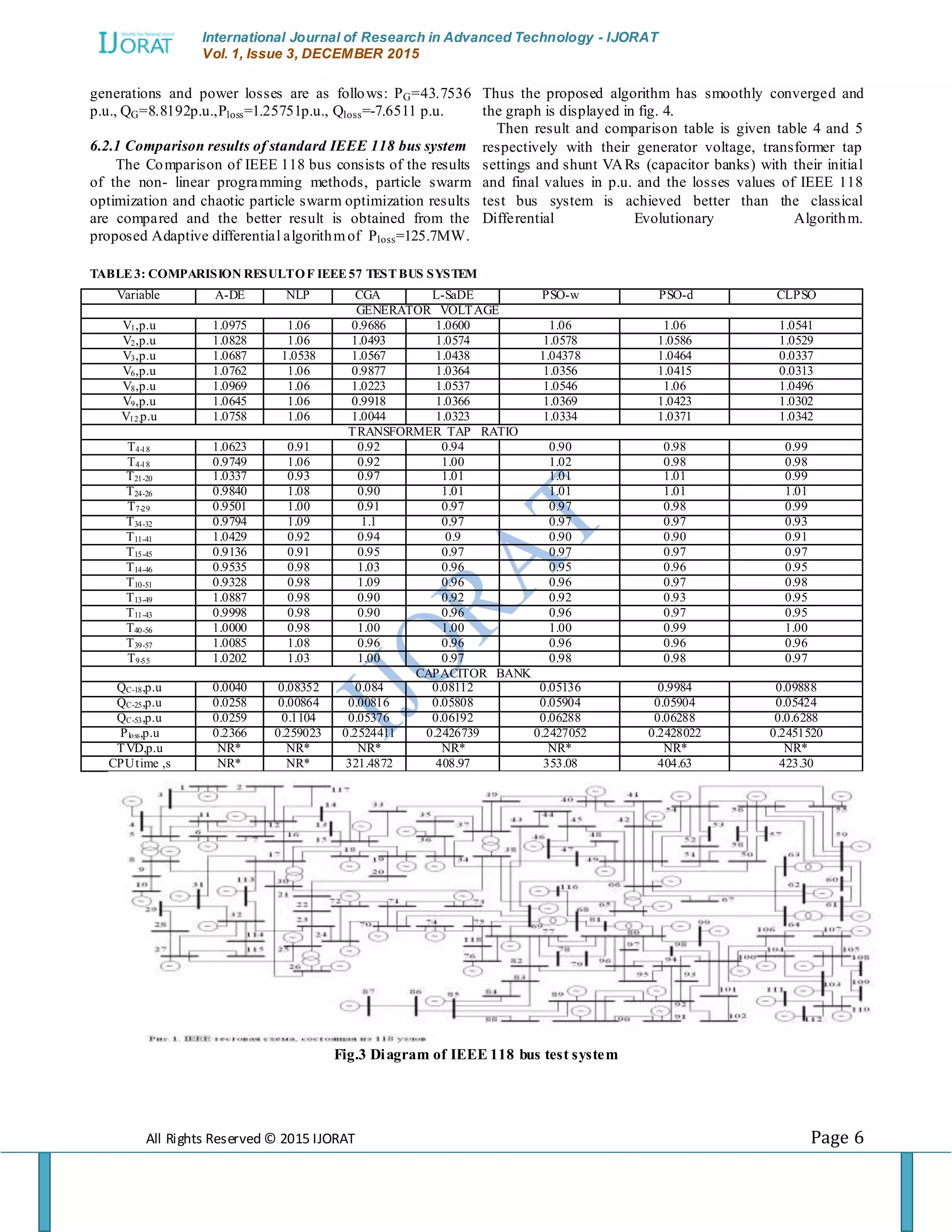
![International Journal of Research in Advanced Technology - IJORAT Vol. 1, Issue 3, DECEMBER 2015 All Rights Reserved © 2015 IJORAT Page 4 stabilizes to a constant value. A very small difference in F1(0) causes the significant difference in its variation pattern. The system at [27] is deterministic and displays chaotic behavior when μ=4 and F(0)€(0,0.25,0.5,0.75,1.0). The mutation parameter F is increased from an initial value F2i to a final value F2f with the iterative progress of the optimization algorithm, as per the dynamics given by [27- 28] by suitable choice of initial and final values of mutation rate. F(t)=[(F2f–F2i)(iter/itermax )+F2i]F1t (21) In the proposed adaptiveDE algorithm, the value of CR is changed iteratively as given below: CR(iter)=(CRmax –Cmin ) (22) IV. IMPLEMENTATION OF ADAPTIVE DE ALGORITHM The proposed Adaptive DE algorithm based approach has been formulated and implemented using matlab. Several trials have been taken with different values of DE key parameters such as differentiation (mutation) constant F, crossover constant CR, size of population NP, and the maximum number of generations (iterations) itermax which is used here as a stopping criteria to find the optimal DE key parameters. The first step in the DE algorithm and Adaptive DE algorithm is creating an initial population. All the independent variables which include generator voltages, transformer tap settings and shunt VAR compensations have to be generated according to [15], where each independent parameter of each individual in the population is assigned a value within its specified feasible region. This creates parent vector of independent variables for the first generation, after finding the independent variables, dependent variables like generator reactive power, and voltages at load buses and line flows were calculated using newton-raphson load flow (NRLF) program. 4.1Computational steps of DE algorithm DE algorithm, SaDE, EPSDE and Adaptive DE have been employed to find the best control variables setting starting from randomly generated initial population. At the end of the each iteration, the best individuals, based on the fitness value, are stored. The computational steps of the proposed DE algorithm are as follows: 1. Generate an initial population randomly within the control variables setting starting from randomly within the control variables lower and upper bounds. 2. For each individual in the population, run NRLF program, to find the operating points. 3. Evaluate the fitness of the individuals. 4. Perform mutation and crossover operation using (16)-(17). 5. Select the individuals for the next generations. 6. Store the best individuals of the current generation. 7.Repeat steps 2-5, till the termination criterion is met. 8.Select the control variables setting corresponding to the overall best individual. 9.If the solution is acceptable, find out the best individual and its objective value. Otherwise, change the settings of DE and repeat the steps 1-8. V. DESCRIPTION OF IEEE TEST BUS SYSTEM The description of the test bus system consists of three buses, namely standard IEEE 30-bus, IEEE 57-bus, and IEEE 118-bus respectively. Each bus is consists of their own generators, transformer tap settings and shunt VAR capacitors with their branches, equality and inequality constraints and base case of control variables and state variables. TABLE 1 description of IEEE test bus system VI. RESULTS AND DISCUSSIONS 6.1 Test Bus system : IEEE 57-bus power system The standard IEEE 57-bus system consists of eighty transmission lines, seven generators (at the buses 1, 2, 3, 6, 8, 9, 12) and fifteen branches under load tap setting transformers branches is taken as test system 1. There reactive power sources are considered at buses 18, 25 and 53. Line data, bus data, variable limits and the initial values of the control variables are considered. The search space of this case systemhas twenty five dimensions, including seven generator voltages, fifteen transformer tap and three reactive power sources. The system loads are given as follows: Pload=12.508 p.u, Qload=3.364p.u. The initial total generations and power losses are: PG=12.7926p.u. ,QG=3.4545p.u. 6.1.1 Comparison results of standard IEEE 57 bus system The Comparison of IEEE 57 bus consists of the results of the non- linear programming methods, particle swarm optimization and chaotic particle swarm optimization results are compared and the better result is obtained from the proposed Adaptive differential algorithmof Ploss=0.2336 p.u TABLE 2: SIMULATION RESULTS OF IEEE 57 BUS TEST SYSTEM description IEEE30 bus IEEE57 bus IEEE 118 bus Buses,NB 30 57 118 Generators,NG 6 7 54 Transformers,NT 4 15 9 Shunts,NQ 9 3 14 Branches,NE 41 80 186 Equality constraints 60 114 236 Inequality constraints 125 245 572 Control variables 19 27 77 State variables 6 20 21 Base case for Ploss,MW 5.660 27.8637 132.4500 Base case for TVD,p.u 0.58217 1.23358 1.439337](https://image.slidesharecdn.com/vol1issue3p001-160121144600/75/An-Adaptive-Differential-Evolution-Algorithm-for-Reactive-Power-Dispatch-4-2048.jpg)
![International Journal of Research in Advanced Technology - IJORAT Vol. 1, Issue 3, DECEMBER 2015 All Rights Reserved © 2015 IJORAT Page 9 promising algorithm for solving some more other complex engineering optimization problem for future researchers. ACKNOWLEDGMENT I would especially like to express my extreme gratitude and sincere thanks to: Dr.A. SHUNMUGALATHAM.E,Ph.d, Professor and Head of the Department, Electrical and Electronics Engineering, Velammal College of Engineering and Technology for her enthusiastic and innovative guidance during the entire period of my project. I would like to express my deep sense of gratitude and heartiest thanks to: My guide MR.T.CHANDRASEKAR M.E, Assistant Professor II, Electrical and Electronics Engineering, Velammal College of Engineering and Technology for her constant source of encouragement and for the valuable guidance. Her moral support encouraged me to process through my work successfully. REFERENCES [1] Abido MA, “Optimal power flow using particle swarm optimization,” Elecric power Energy Syst 2002:24(7):563-571. [2] Dommel HW,Tinney WF, “Optimal power flow solutions,” IEEE Trans power apparatus Syst 1968:1866-1876. [3] Durairaj S,kannan PS, Devaraj D, “ Multi-objective VAR dispatch using particle swarm optimization”,EmergElect power Syst 2005:4. [4] Abido MA,Bakshawain JM,” Optimal VAR dispatch using a multi- objective evolutionary algorithm”, In: IEEE congress on evolutionary computation,” van cover, BC, Canada:2006. P. 730-736. [5] Abido MA,” Multi-objective VAR dispatch using strength pareto evolutionary algorithm” W.-K. Chen, Linear Networks and Systems, Belmont, CA: Wadsworth, 1993, pp. 123-135. [6] Lee KY, Park YM, Ortiz JL”A united approach to optimal real and reactive power dispatch”, IEEE Trans power apparatus Syst PAS 1985:104(5):1147-1153. [7] Granville s,” Optimal reactive power dispatch through interior point methods”,IEEE Trans power Syst 1994:9(1):98-105. [8] Mansour MO, Abdel-Rahaman TM,” Non-linear VAR optimization using decomposition and coordination”,IEEE Trans power apparatus Syst PAS1984:103(2):246-255. [9] Mamandur KRC, Chenweth RD,” Optimal control of reactive power flow for improvements in voltage profiles and for real power loss minimization”,IEEE Trans power apparatus Syst PAS 1981:100(7):3185-3193. [10] Roy PK, Ghoshal SP, Thakur SS,” Optimal VAR for improvements in voltage profiles and for real power loss minimization using biogeography based optimization”, Electric Power Energy Syst 199:10(3):1243-9. [11] Iba k,” Reactive power optimization by genetic algorithm”,IEEE Transpower Syst 1994:9(2):685-692. [12] Wu QH, Ma JT,” Power system optimal reactive power dispatch using evolutionary programming”,IEEE Trans power apparatus Syst 1995:10(3):1243-1249. [13] Lai LL, MA JT,” Application of evolutionary programming to reactive power planning-comparison with nonlinear programming approach”,IEEE Trans power Syst 1997:12(7):198-206. [14] Swain AK, Morries AK“A novel hybrid evolutionary programming method for function optimization”, In: proc congress on evolutionary computation, Vol. 1:2000, p.699-705. [15] Das Bhagwan D, Patvardhan c,” A new hybrid evolutionary strategy for reactive power dispatch”, IEEE Trans power Syst Res 2003;65:83-90. 1995:10(3):1243-1249. [16] Yoshida H, Kawata K, Fukuyama S, Nakanishi Y,” A particle swarm optimization for reactive power and voltage control considering voltage security assessment”,IEEE Trans power Syst 2000:15(4):1232-1239. [17] Esmin AAA, Lambert-Torres G, de souza ACZ,” A hybrid particle swarm optimization appliedto loss power minimization”,IEEE Trans power Syst 2005:20(2):859-866. [18] AbouELEla, Abido MA, Spea SR, “ Differential evolution algorithm for optimal reactive power dispatch”,IEEE Trans power Syst Res 2011:81:458-464. [19] Vardarajan M, Swarup KS,” Differential evolution for optimal reactive power dispatch”, IEEE Trans power Energy Syst 2008;30:435-441. [20] BadarAltaf QH, Urme BS, Jungre AS,” Reactive power control using dynamic particle swarm optimization for real power loss minimization”, Int J Electric Power Energy Syst 2012;41:133-136. [21] Li Yuancheng, Wang Yiliyang Li Bin,” A hybrid artificial bee colony assisted differential evolutionary algorithm for optimal reactive power flow”,Int J Electric power Energy Syst 2013;52:25- 33. [22] Chaturvedi KT, Pandit M, Srivastava I,” Self-organizing hierarchical particle swarm optimization for non-convex economic dispatch”,Roy PK, Ghoshal SP, Thakur SS,” Optimal VAR for improvements in voltage profiles and for real power loss minimization using biogeography based optimization”, IEEE Trans Power Syst 2008;23(3):1079-1087. [23] Pandit M, Srivastava L, Pal K,” Static/dynamic optimal dispatch of energy and reserveusing recurrent differential evolution,” to appear in IET proceedings- GenerTrasmDistri, doi:10.1049/iet- gtd.2013.0127.ISSN1751-8687. [24] Storn R, Price K,” Differential evolution- a simple and efficient heuristic for global optimization over continuous spaces”, Tech Report TR-95-012,ICSI;1995. [25] Storn R, Price K,” Differential evolution- a simple and efficient heuristic for global optimization over continuous spaces”, J global optim 1997;11: 34-359. [26] Vesterstrom J, Thomsen R,” A comparative study of differential evolution, particle swarm optimization and evolutionary algorithm: on numerical benchmark problems,” In; IEEE congress on evolutionary computation:2004. p. 90-987. [27] Das S, Abrham A, Konar A,” particle swarm optimization and differential evolutionary algorithms: technical analysis, applications and hybridization perspectives. <http;//www.softcomputing.net/aciis.pdf>. [28] Yang Zhenyu, Tang KE, Yao Xin,”Differential evolution for high dimensional function optimization‟, In IEEE congress on, Evolutionary computation (CEC2007); p.3523-3530. [29] Vaisakh K, KantaRao P,‟ differential evolution based optimal power dispatch for voltage stability enhancement „, J theorAppl Inform Technol 2008; 638- 646. [30] Balamurugan R, Suramanian S,” Self adaptive differential evolution based power dispatch of generators with valve-point effects and multiple fuel options”. computingSciEng 2007;1:10-17. [31] Arya LD, Singh Pushpendra, Titare LS,” Anticipatory reactive power reserve maximization using differential evolution. Int J Electric Power Energy Syst 2012;35:66-73. [32] Arya LD, Singh Pushpendra, Titare LS,” Optimum load shedding based on sensitivity to enhance static voltage stability using DE”, Swarm EvolutComput 2012;6:25-38. [33] Kalanmony Deb,” multi-objective optimization using evolutionary algorithm”, John wiley& Sons Ltd.2010. [34] Qin AK, Huang VL, Suganthan PN,” Differential algorithm with strategy adaptation for global numerical optimization”, IEEE Trans EvolutComput 2009;13(2):398-417. [35] Mallipeddi R, Suganthan PN, Pan QK, Tasgetiren MF,” Differential algorithm with ensemble of parameters and mutation strategies”, Appl Soft Comput 2011;11(2):1679-1696. [36] Yu G, Wang X, Li P,” Application of chaotic theory in differential evolution algorithms”, In : proceedings of international conference on natural Coputation (ICNC);2010. P. 3816-3820. [37] Capnetto R, ForttunaFazzino S, XibiliaMG,‟Chaotic sequences to improve the performance of evolutionary algorithms”, IEEE Trans EvolutComput 2003;7(3):289-304. [38] Coelho R, Mariani VC,” Combining of Chaotic differential evolution and quadratic programming for economic dispatch optimization with valve point effect”, IEEE Trans Power Syst 2006;21(2):989-996.](https://image.slidesharecdn.com/vol1issue3p001-160121144600/75/An-Adaptive-Differential-Evolution-Algorithm-for-Reactive-Power-Dispatch-9-2048.jpg)
![International Journal of Research in Advanced Technology - IJORAT Vol. 1, Issue 3, DECEMBER 2015 All Rights Reserved © 2015 IJORAT Page 10 [39] He D, Dong G, Wang F, Mao Z,” optimization of dynamic economic dispatch with valve point effect using chaotic sequence based differential evolution algorithms”, Energy Convers Manage 2011;52(2):1026-1032. [40] Pal Kirti, Pandit M, Srivastava L,” Joint energy and reserve dispatch in a multi-area competitive market using time varying differential evolution”, Int J EngSciTechnol (IJEST)2011;3(1):87-10. [41] StandardIEEE 57 Test Bus System. [42] StandardIEEE 118 Test Bus System.](https://image.slidesharecdn.com/vol1issue3p001-160121144600/75/An-Adaptive-Differential-Evolution-Algorithm-for-Reactive-Power-Dispatch-10-2048.jpg)

This document summarizes an adaptive differential evolution algorithm for solving the reactive power dispatch problem, which involves minimizing real power losses. The problem is formulated as a non-linear constrained optimization problem. An adaptive differential evolution algorithm is proposed that uses time-varying chaotic mutation and crossover to avoid parameter tuning. The algorithm is applied to the IEEE 57-bus and 118-bus test systems and found to provide superior convergence and solution quality compared to classical differential evolution and self-adaptive differential evolution algorithms.