Algorithmic Data Science = Theory + Practice

Algorithmic Data Science = Theory + Practice Matteo Riondato – Labs, Two Sigma Investments @teorionda – http://matteo.rionda.to IEEE MIT URTC – November 5, 2016 1 / 24

Matteo Riondato Ph.D. in CS Working at Labs, Two Sigma Investments (Research Scientist); CS Dept., Brown U. (Visiting Asst. Prof.); Doing research on algorithmic data science; Tweeting @teorionda; Reading matteo@twosigma.com; “Living” at http://matteo.rionda.to. 2 / 24

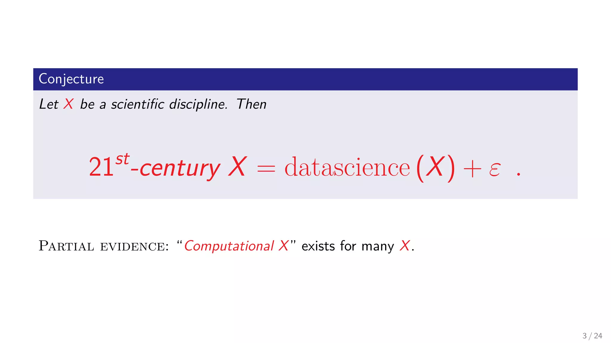
Conjecture Let X be a scientiﬁc discipline. Then 21st -century X = datascience (X) + ε . Partial evidence: “Computational X” exists for many X. 3 / 24

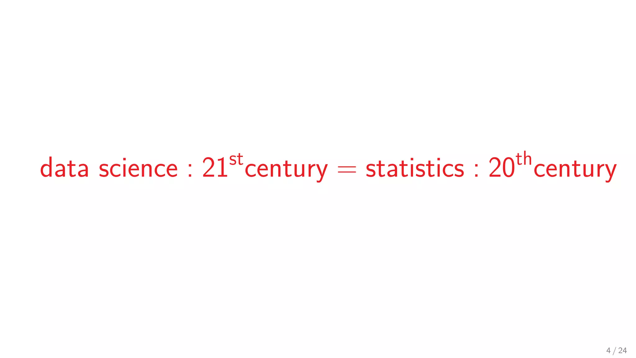
data science : 21st century = statistics : 20th century 4 / 24

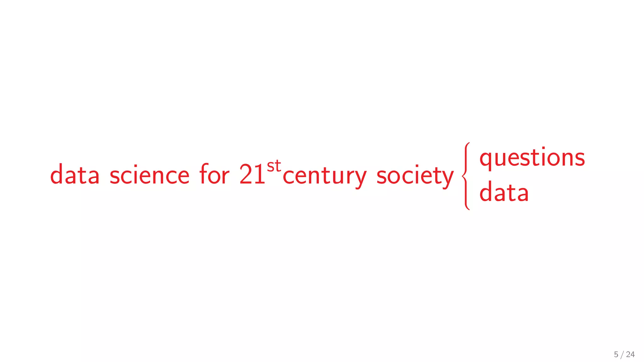
data science for 21st century society    questions data 5 / 24

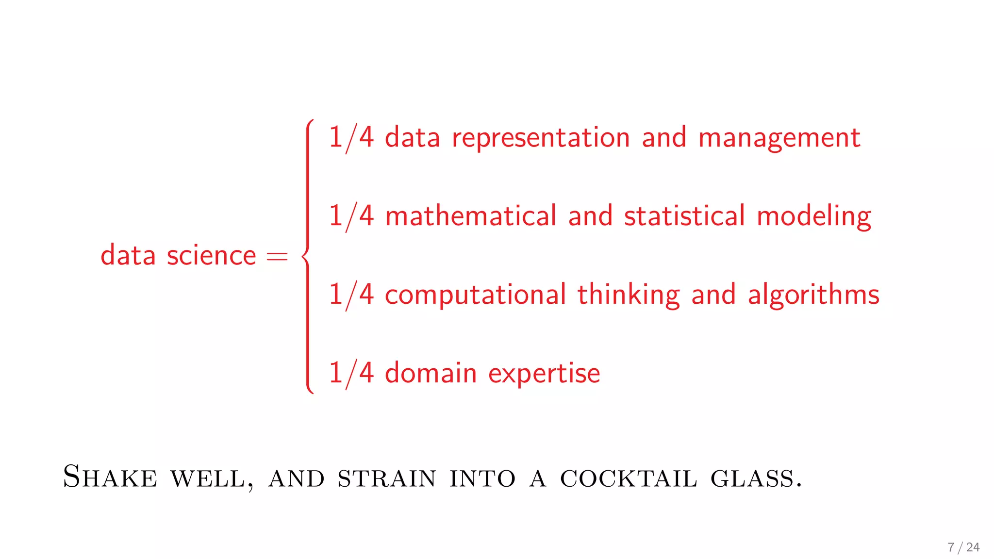
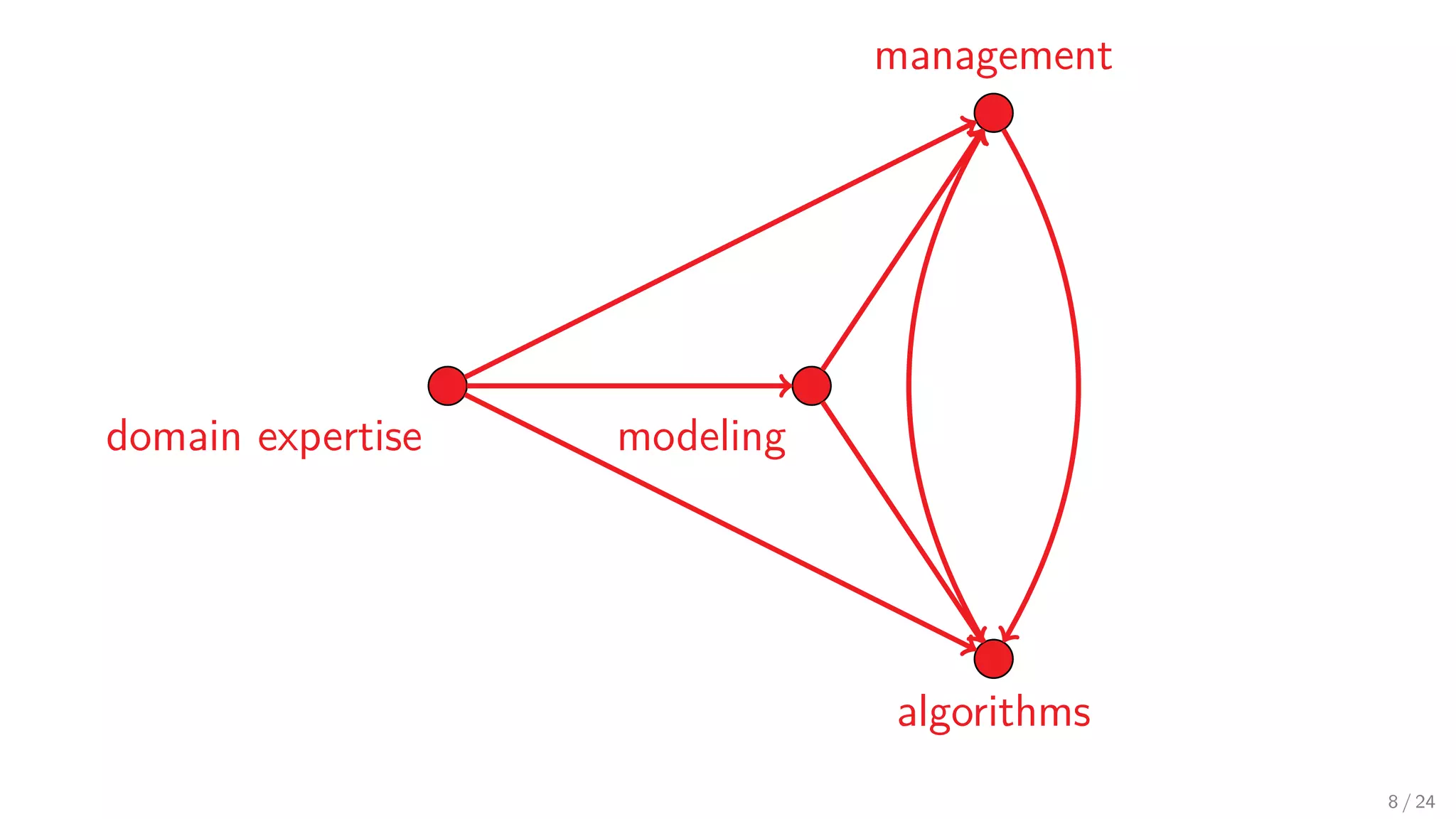
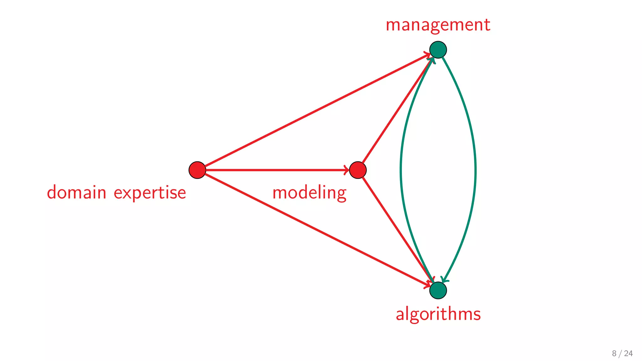
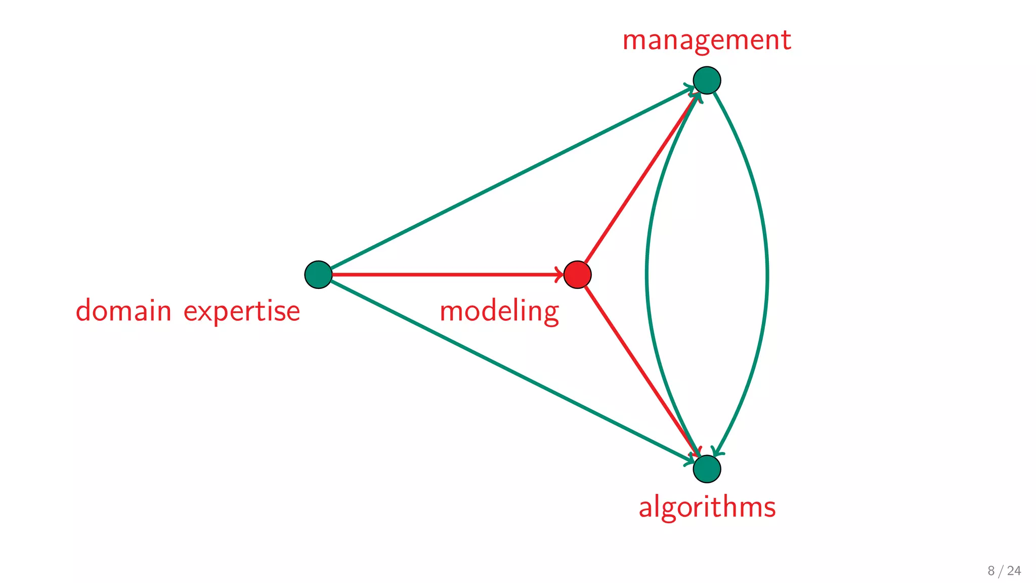
data science =    1/4 data representation and management 1/4 mathematical and statistical modeling 1/4 computational thinking and algorithms 1/4 domain expertise Shake well, and strain into a cocktail glass. 7 / 24

domain expertise modeling management algorithms 8 / 24

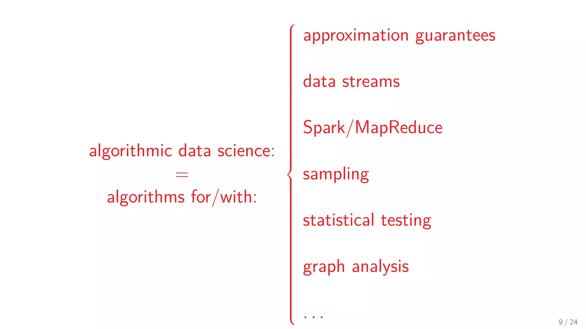
algorithmic data science: = algorithms for/with:    approximation guarantees data streams Spark/MapReduce sampling statistical testing graph analysis . . . 9 / 24

algorithmic data science = theory 10 / 24

algorithmic data science ≈ theory + practice 10 / 24

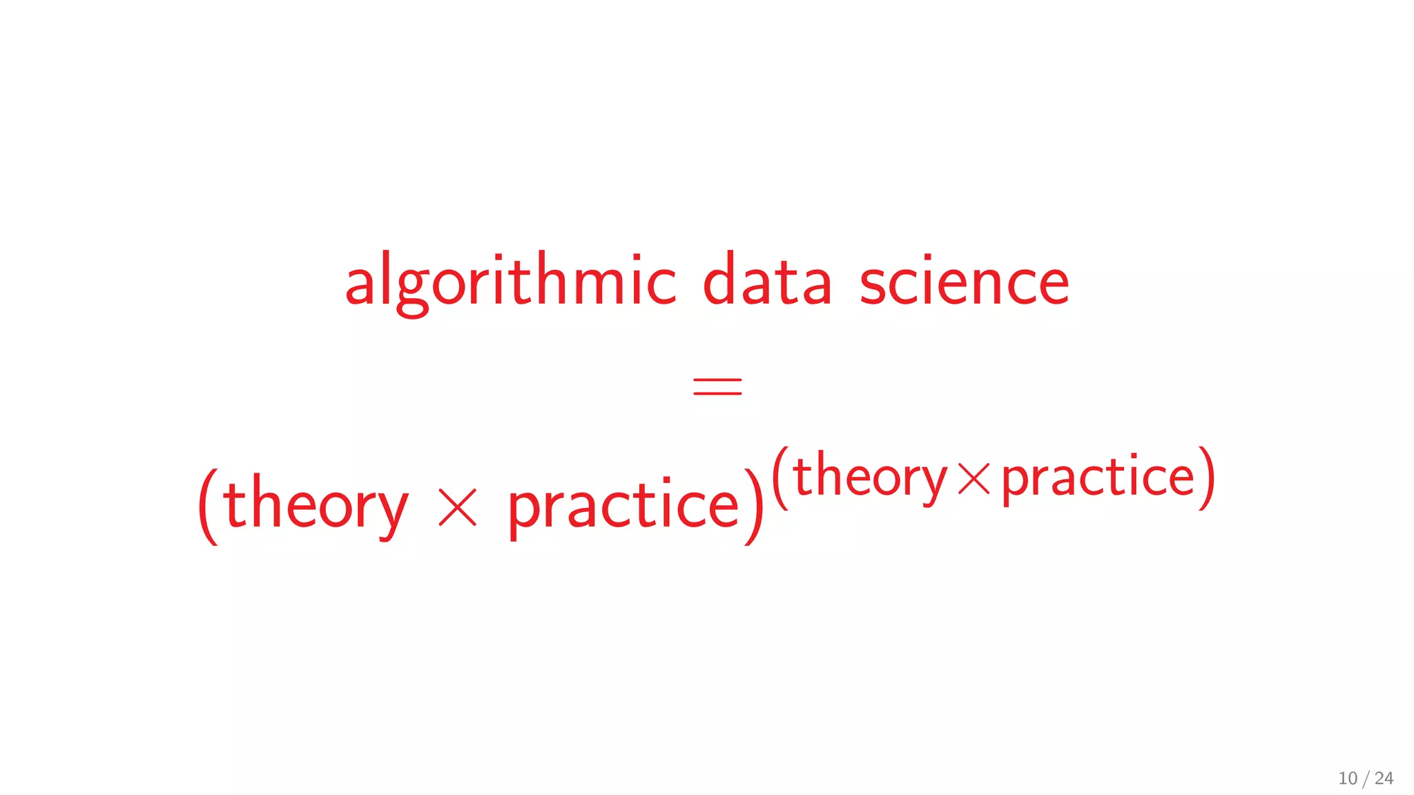
algorithmic data science = (theory × practice)(theory×practice) 10 / 24

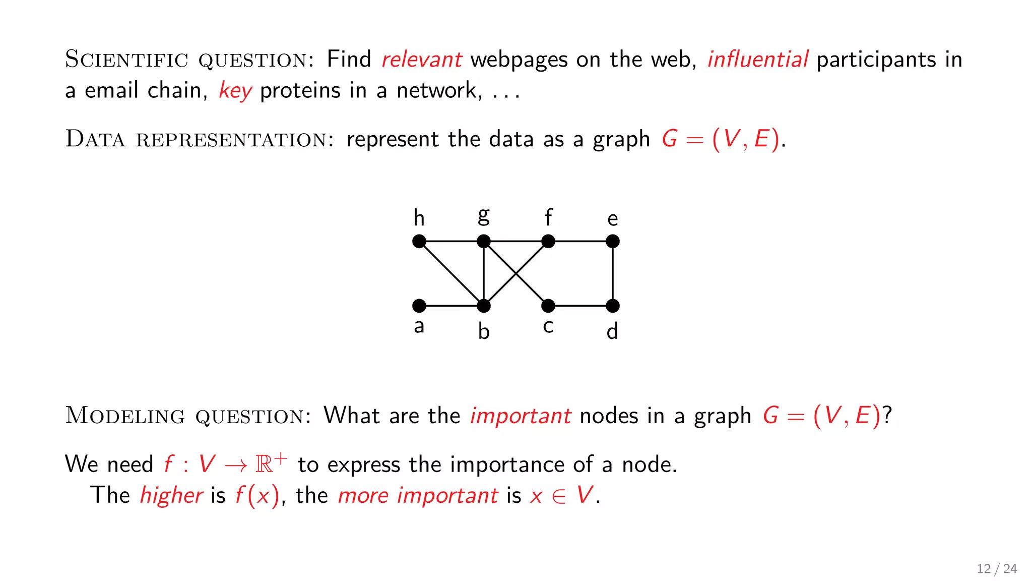
Scientific question: Find relevant webpages on the web, inﬂuential participants in a email chain, key proteins in a network, . . . Data representation: represent the data as a graph G = (V , E). a h b g f e c d Modeling question: What are the important nodes in a graph G = (V , E)? We need f : V → R+ to express the importance of a node. The higher is f (x), the more important is x ∈ V . 12 / 24

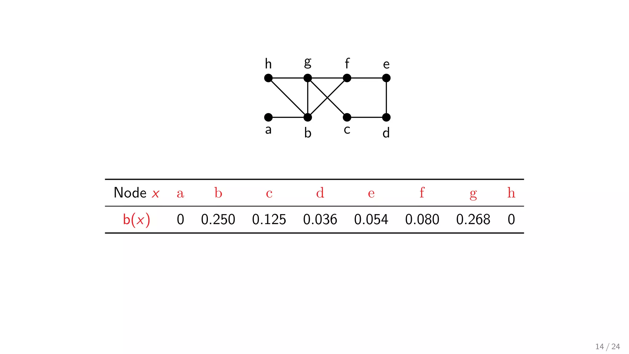
Domain Knowledge / Modeling: Assume that 1) every node wants to communicate with every node; and 2) communication progresses along Shortest Paths (SPs). Then, the higher the no. of SPs that a node v belongs to, the more important v is. Deﬁnition For each node x ∈ V , the betweeness b(x) of x is: b(x) = 1 n(n − 1) u=x=v∈V σuv (x) σuv ∈ [0, 1] • σuv : number of SPs from u to v, u, v ∈ V ; • σuv (x): number of SPs from u to v that go through x. I.e., b(x) is weighted fraction of SPs that go through x, among all SPs in G. 13 / 24

a h b g f e c d Node x a b c d e f g h b(x) 0 0.250 0.125 0.036 0.054 0.080 0.268 0 14 / 24

Algorithmic question: How to compute all b(x)? 15 / 24

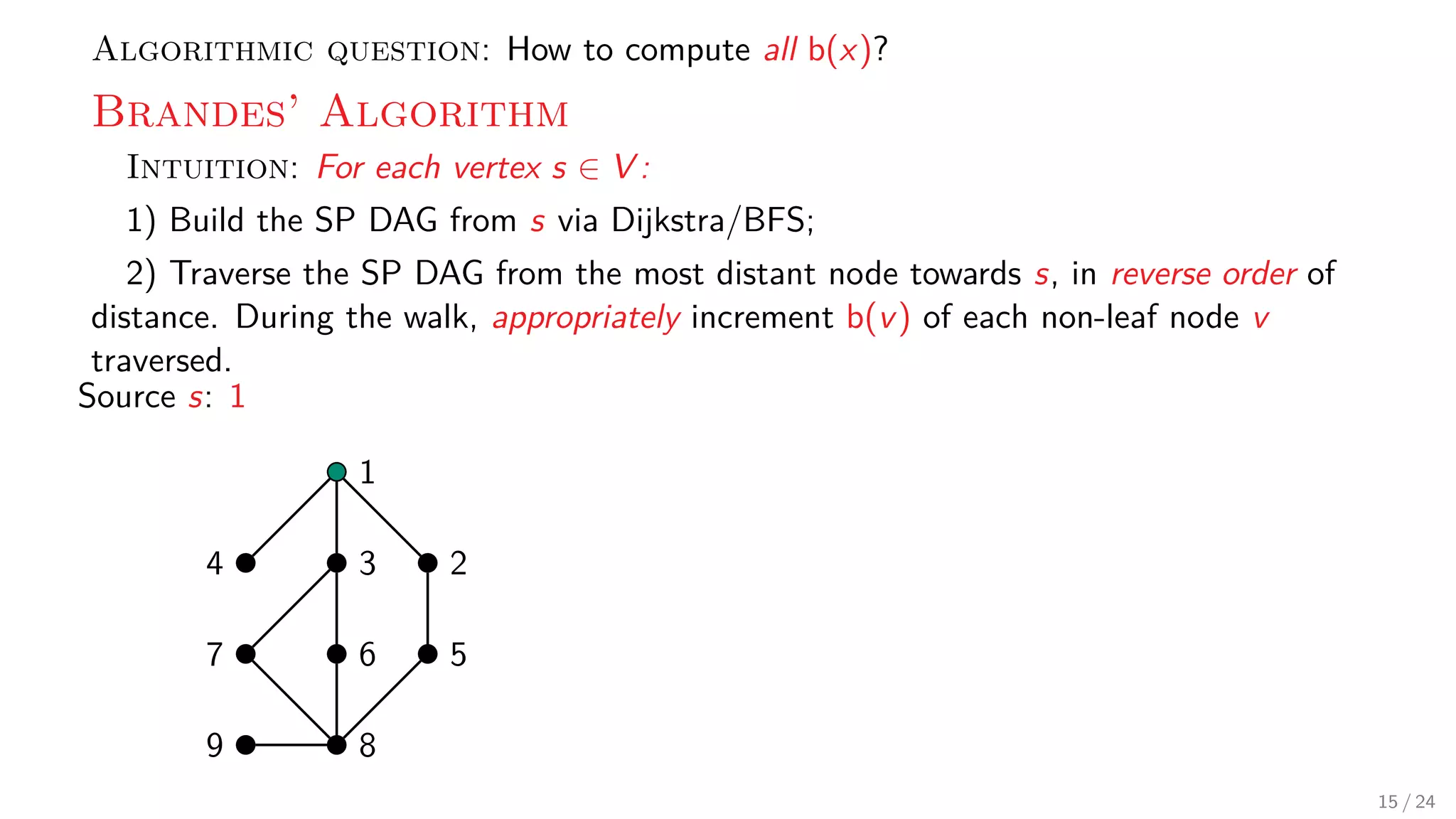
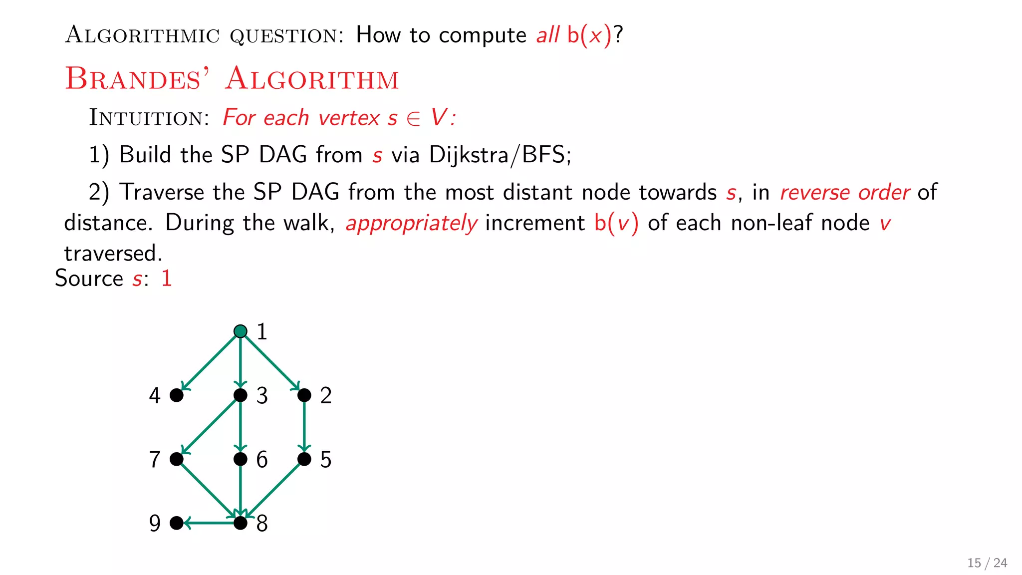
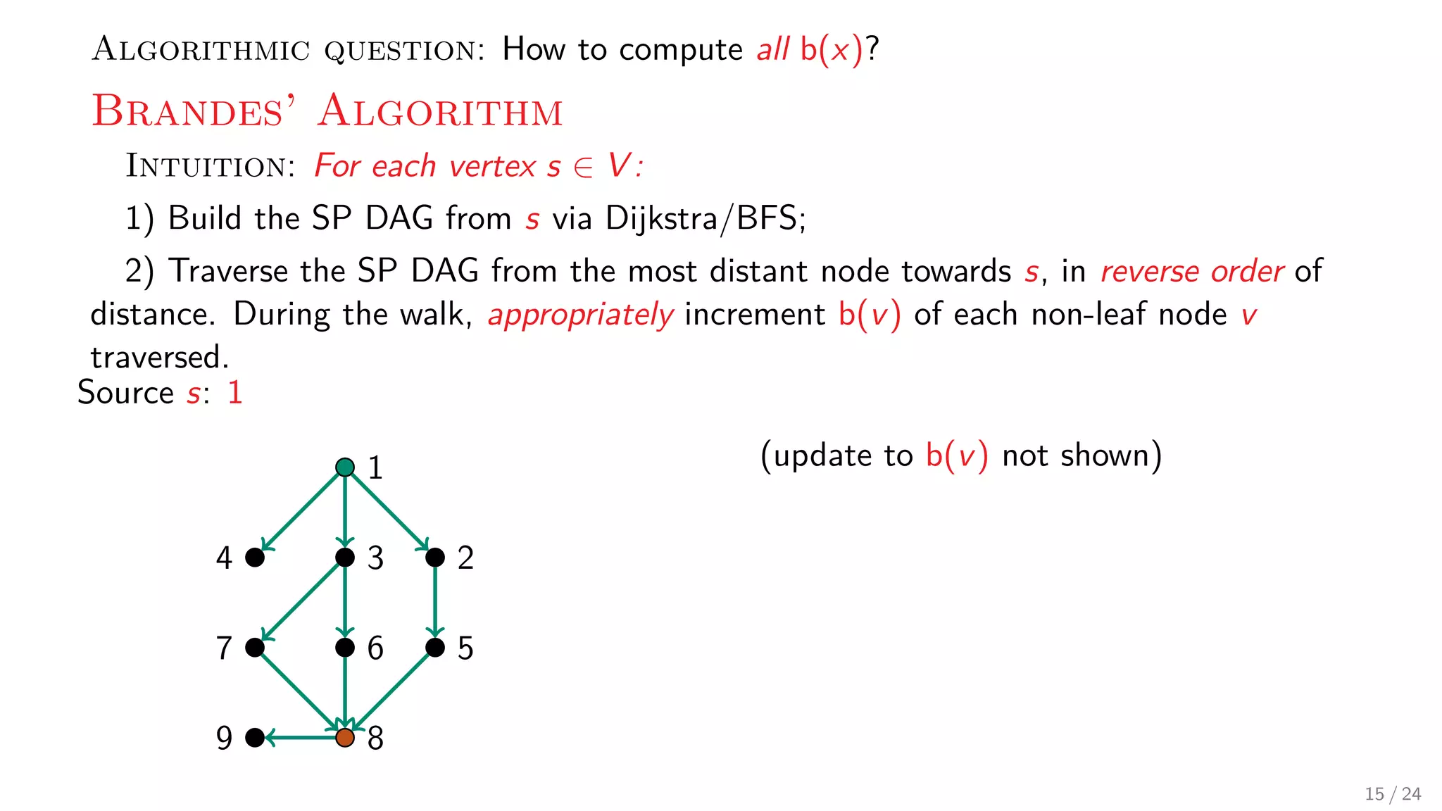
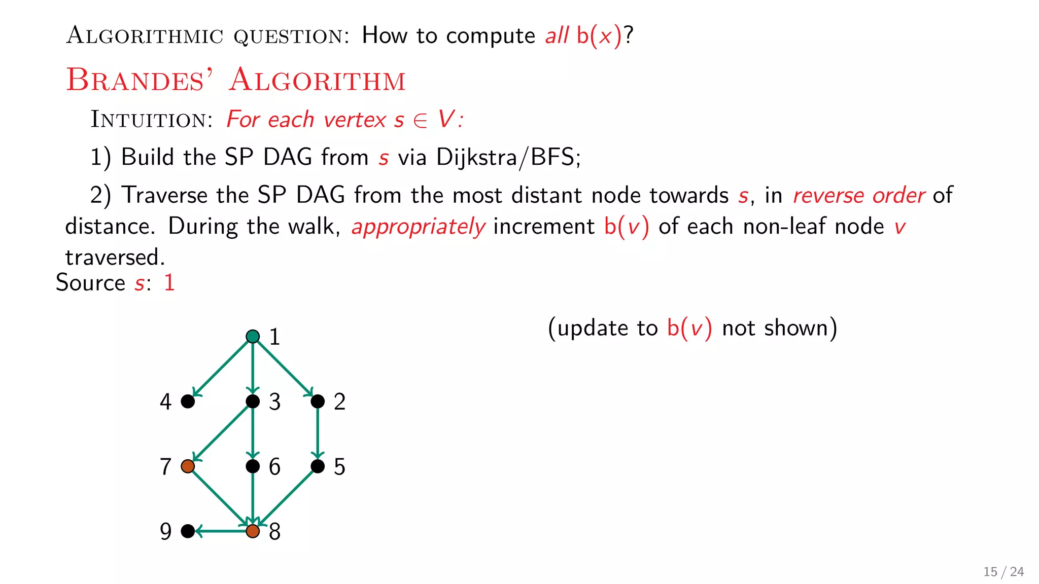
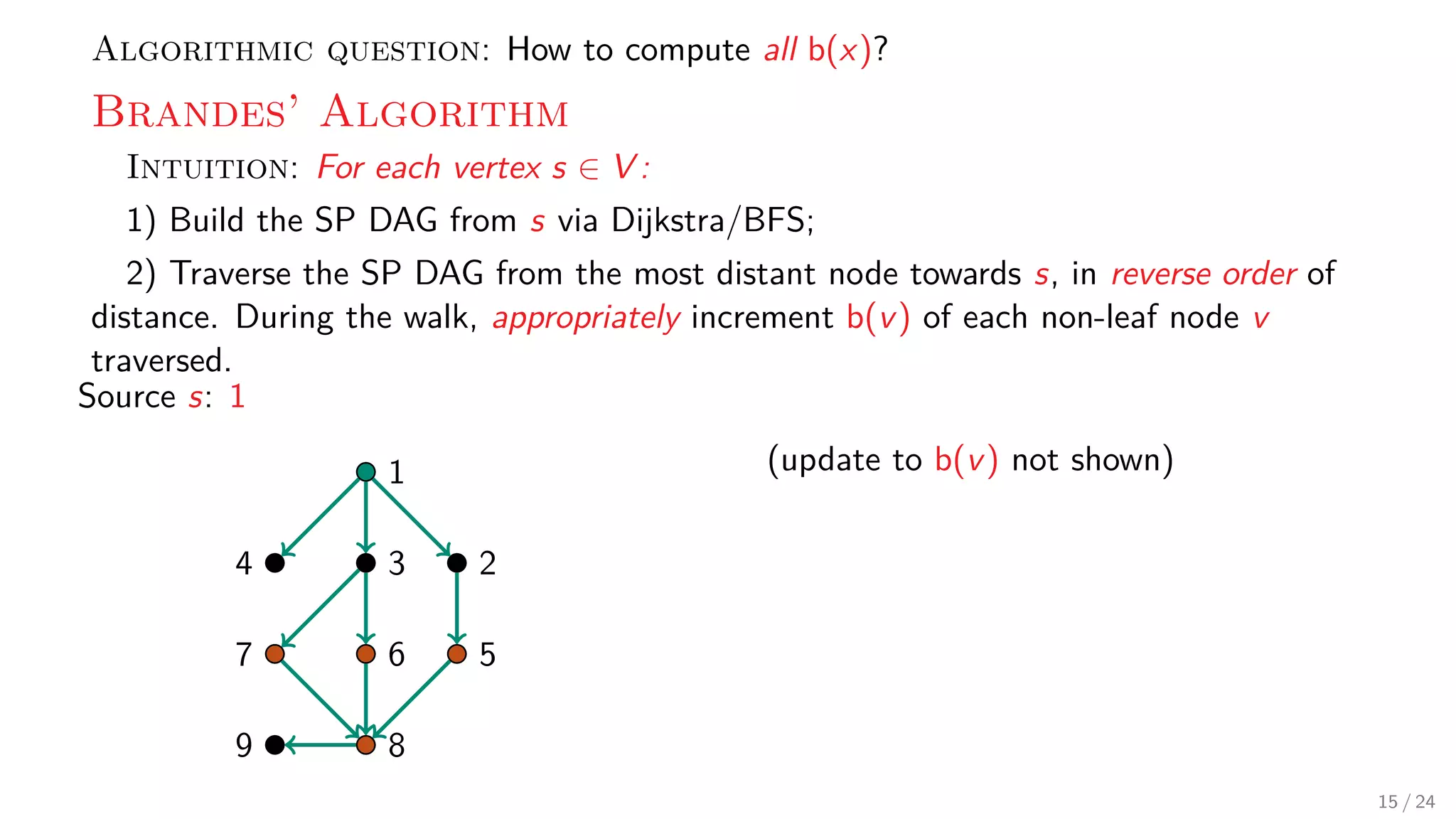
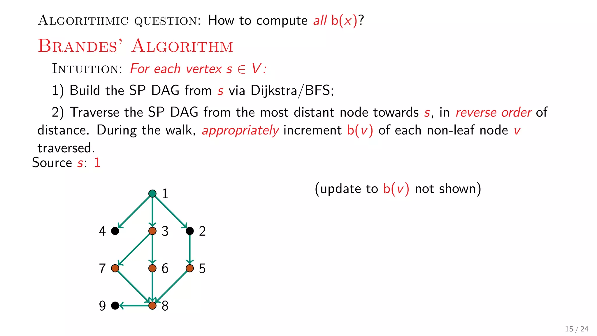
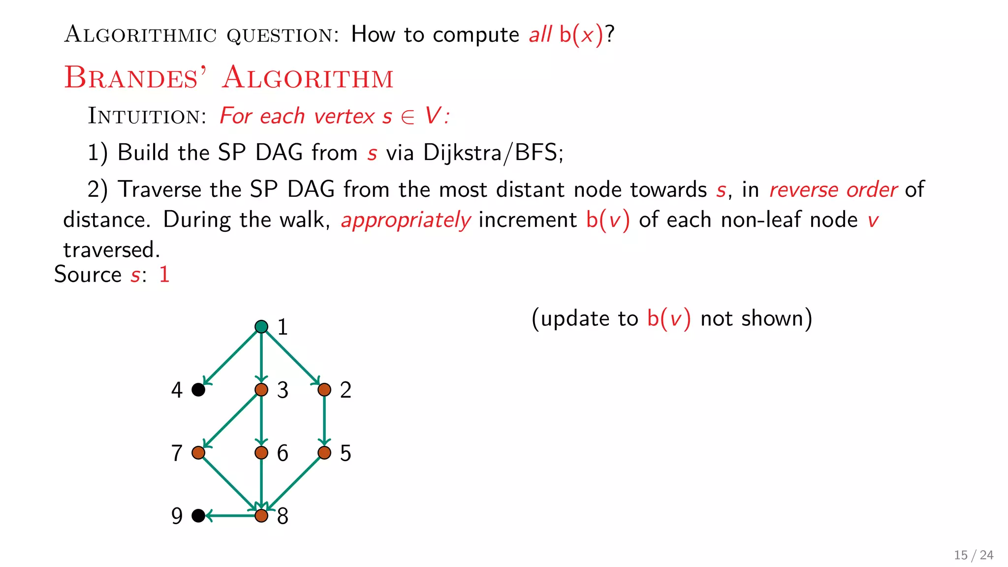
Algorithmic question: How to compute all b(x)? Brandes’ Algorithm Intuition: For each vertex s ∈ V : 1) Build the SP DAG from s via Dijkstra/BFS; 2) Traverse the SP DAG from the most distant node towards s, in reverse order of distance. During the walk, appropriately increment b(v) of each non-leaf node v traversed. Source s: 1 1 234 567 89 15 / 24

Algorithmic question: How to compute all b(x)? Brandes’ Algorithm Intuition: For each vertex s ∈ V : 1) Build the SP DAG from s via Dijkstra/BFS; 2) Traverse the SP DAG from the most distant node towards s, in reverse order of distance. During the walk, appropriately increment b(v) of each non-leaf node v traversed. Source s: 1 1 234 567 89 (update to b(v) not shown) 15 / 24

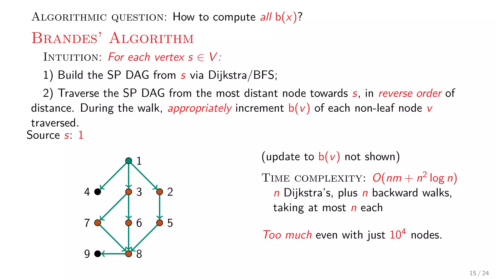
Algorithmic question: How to compute all b(x)? Brandes’ Algorithm Intuition: For each vertex s ∈ V : 1) Build the SP DAG from s via Dijkstra/BFS; 2) Traverse the SP DAG from the most distant node towards s, in reverse order of distance. During the walk, appropriately increment b(v) of each non-leaf node v traversed. Source s: 1 1 234 567 89 (update to b(v) not shown) Time complexity: O(nm + n2 log n) n Dijkstra’s, plus n backward walks, taking at most n each Too much even with just 104 nodes. 15 / 24

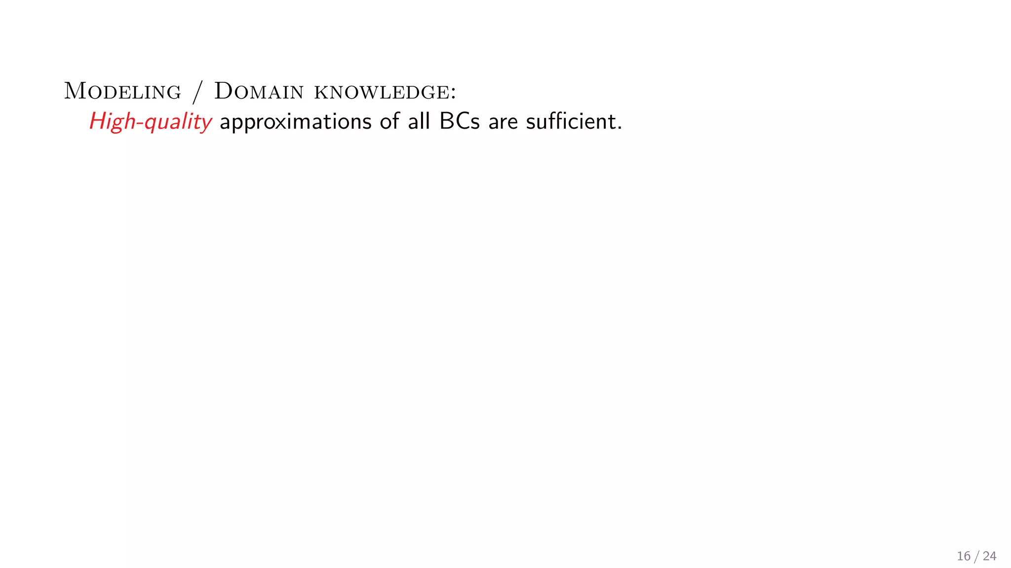
Modeling / Domain knowledge: High-quality approximations of all BCs are suﬃcient. 16 / 24

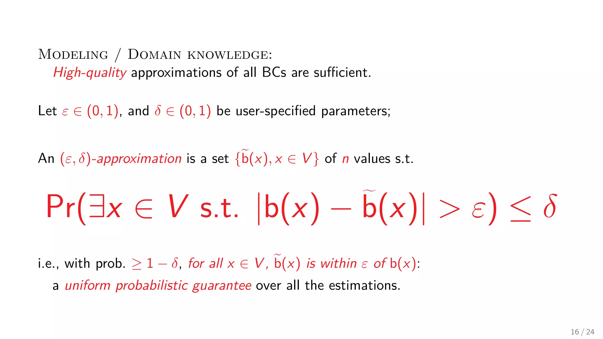
Modeling / Domain knowledge: High-quality approximations of all BCs are suﬃcient. Let ε ∈ (0, 1), and δ ∈ (0, 1) be user-speciﬁed parameters; An (ε, δ)-approximation is a set {b(x), x ∈ V } of n values s.t. Pr(∃x ∈ V s.t. |b(x) − b(x)| > ε) ≤ δ i.e., with prob. ≥ 1 − δ, for all x ∈ V , b(x) is within ε of b(x): a uniform probabilistic guarantee over all the estimations. 16 / 24

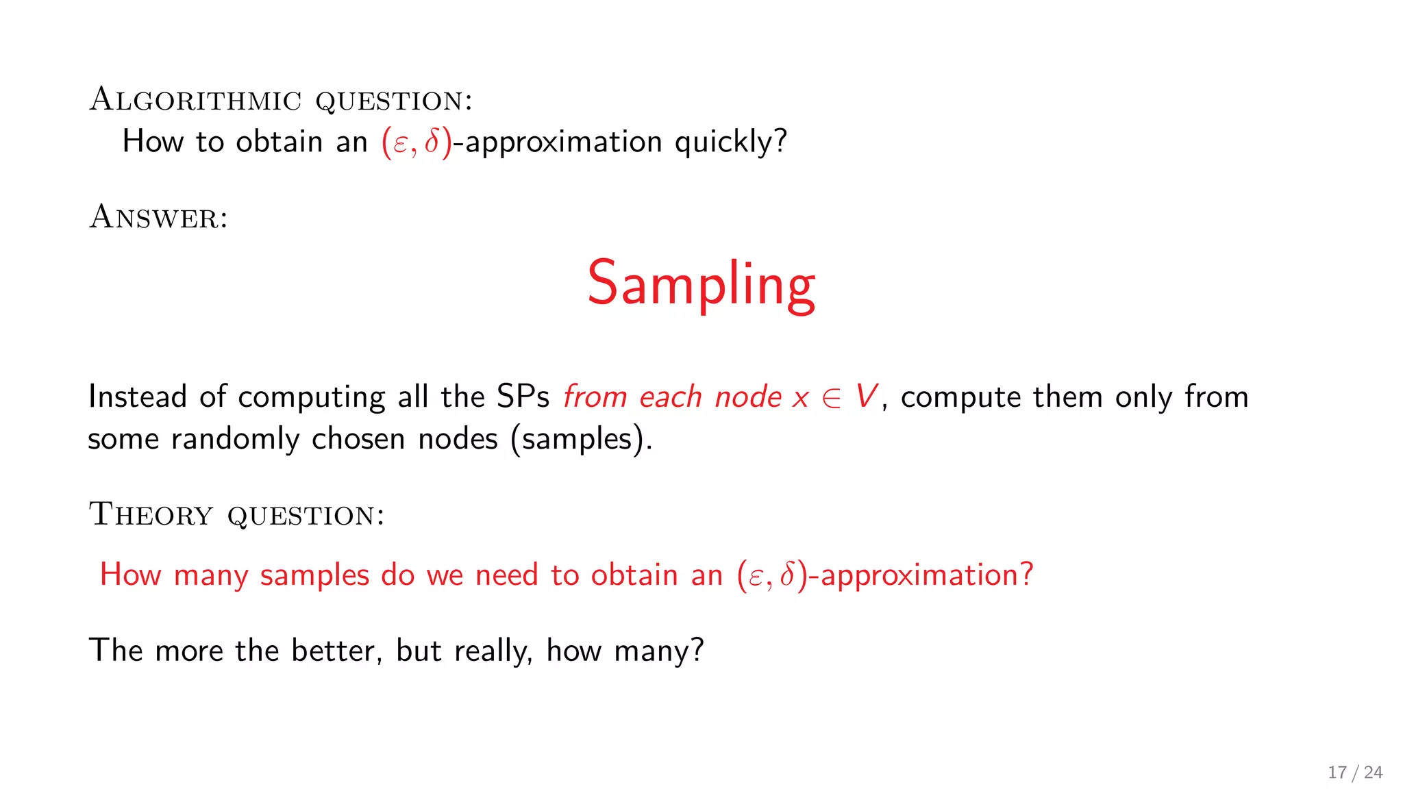
Algorithmic question: How to obtain an (ε, δ)-approximation quickly? Answer: Sampling Instead of computing all the SPs from each node x ∈ V , compute them only from some randomly chosen nodes (samples). Theory question: How many samples do we need to obtain an (ε, δ)-approximation? The more the better, but really, how many? 17 / 24

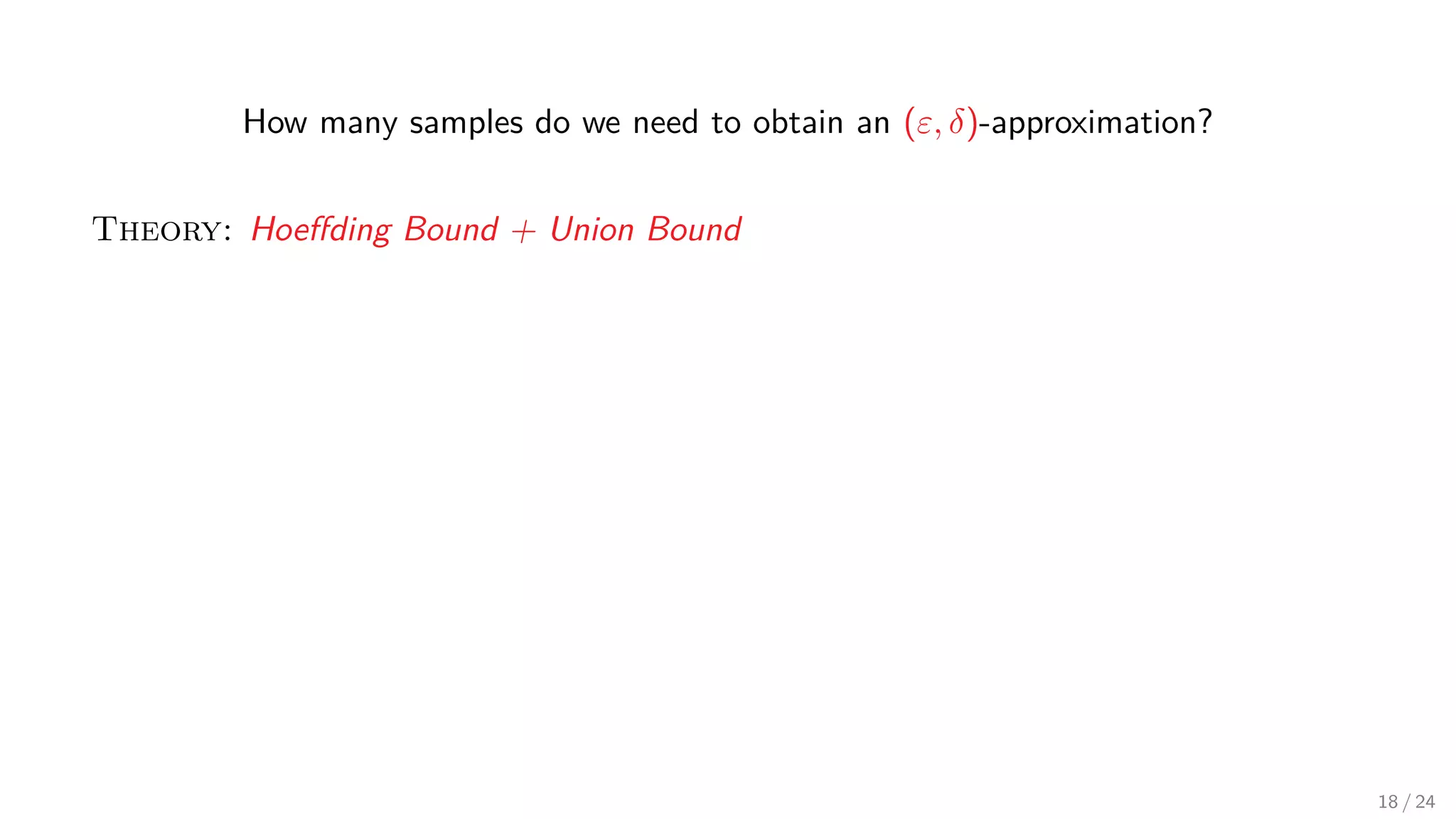
How many samples do we need to obtain an (ε, δ)-approximation? Theory: Hoeﬀding Bound + Union Bound 18 / 24

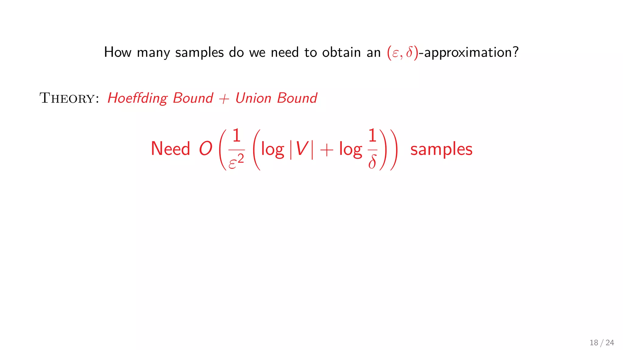
How many samples do we need to obtain an (ε, δ)-approximation? Theory: Hoeﬀding Bound + Union Bound Need O 1 ε2 log |V | + log 1 δ samples 18 / 24

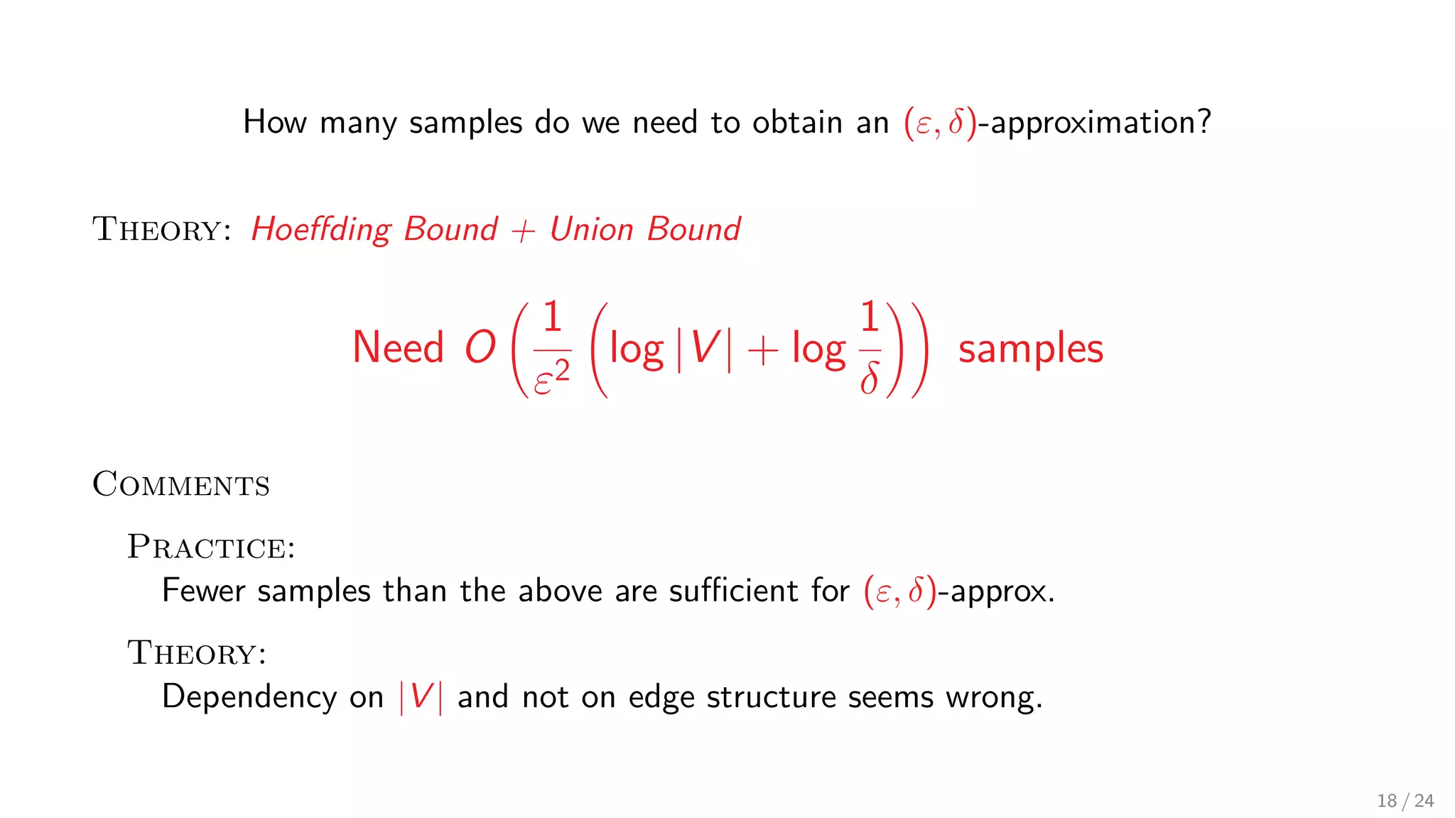
How many samples do we need to obtain an (ε, δ)-approximation? Theory: Hoeﬀding Bound + Union Bound Need O 1 ε2 log |V | + log 1 δ samples Comments Practice: Fewer samples than the above are suﬃcient for (ε, δ)-approx. Theory: Dependency on |V | and not on edge structure seems wrong. 18 / 24

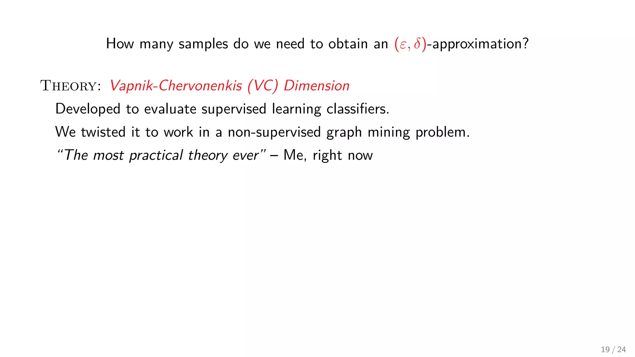
How many samples do we need to obtain an (ε, δ)-approximation? Theory: Vapnik-Chervonenkis (VC) Dimension Developed to evaluate supervised learning classiﬁers. We twisted it to work in a non-supervised graph mining problem. “The most practical theory ever” – Me, right now 19 / 24

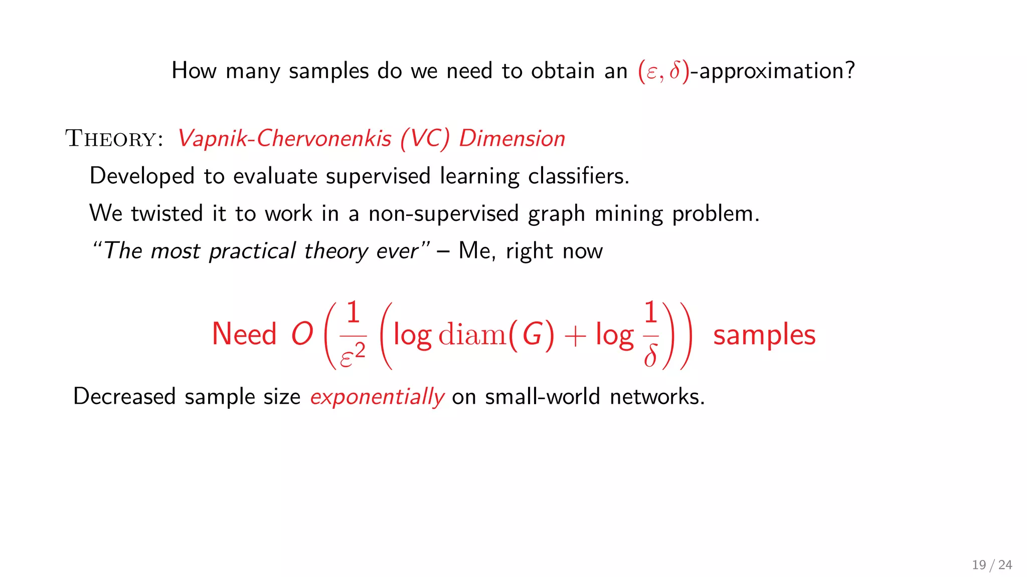
How many samples do we need to obtain an (ε, δ)-approximation? Theory: Vapnik-Chervonenkis (VC) Dimension Developed to evaluate supervised learning classiﬁers. We twisted it to work in a non-supervised graph mining problem. “The most practical theory ever” – Me, right now Need O 1 ε2 log diam(G) + log 1 δ samples Decreased sample size exponentially on small-world networks. 19 / 24

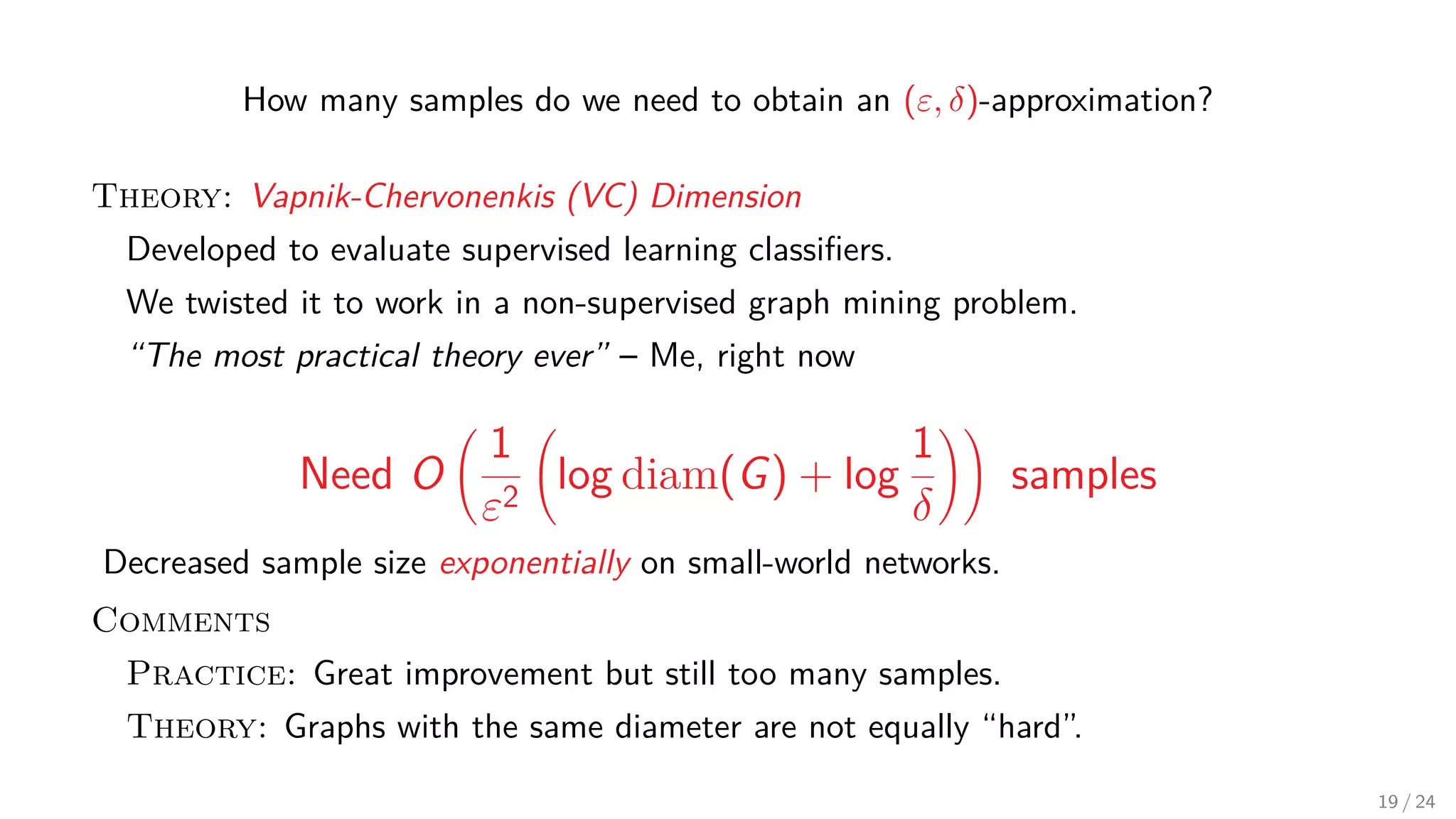
How many samples do we need to obtain an (ε, δ)-approximation? Theory: Vapnik-Chervonenkis (VC) Dimension Developed to evaluate supervised learning classiﬁers. We twisted it to work in a non-supervised graph mining problem. “The most practical theory ever” – Me, right now Need O 1 ε2 log diam(G) + log 1 δ samples Decreased sample size exponentially on small-world networks. Comments Practice: Great improvement but still too many samples. Theory: Graphs with the same diameter are not equally “hard”. 19 / 24

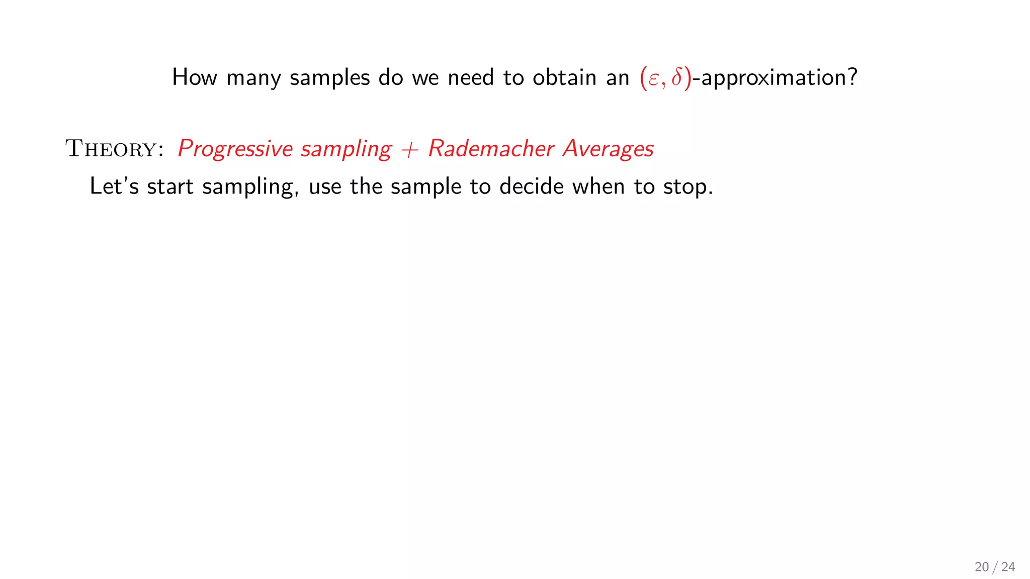
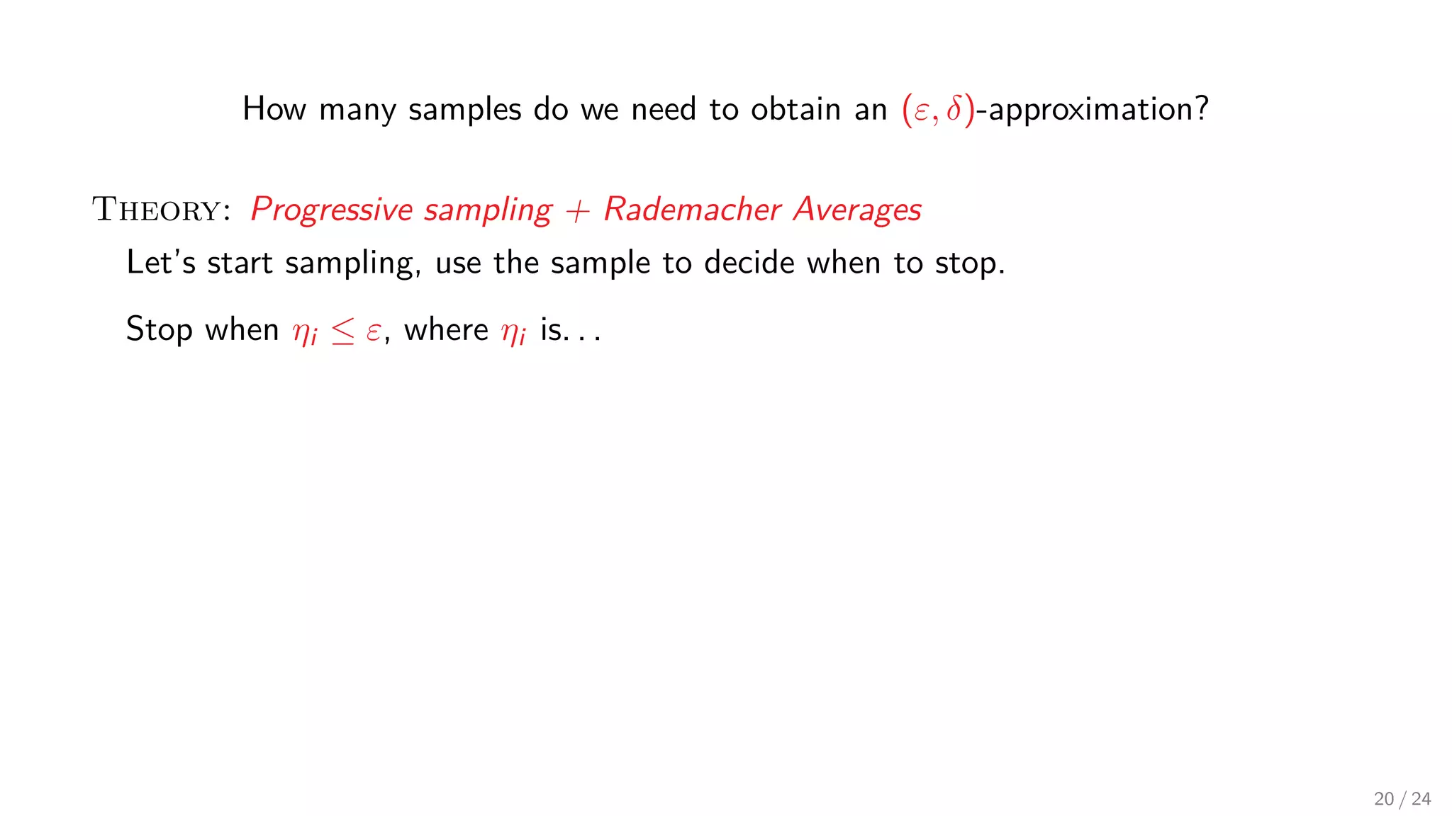
How many samples do we need to obtain an (ε, δ)-approximation? Theory: Progressive sampling + Rademacher Averages Let’s start sampling, use the sample to decide when to stop. 20 / 24

How many samples do we need to obtain an (ε, δ)-approximation? Theory: Progressive sampling + Rademacher Averages Let’s start sampling, use the sample to decide when to stop. Stop when ηi ≤ ε, where ηi is. . . 20 / 24

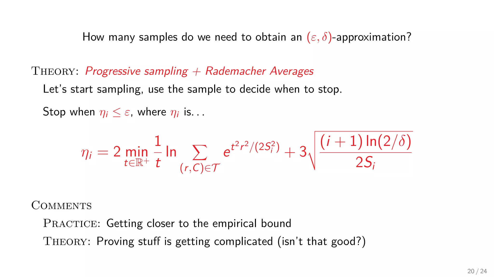
How many samples do we need to obtain an (ε, δ)-approximation? Theory: Progressive sampling + Rademacher Averages Let’s start sampling, use the sample to decide when to stop. Stop when ηi ≤ ε, where ηi is. . . ηi = 2 min t∈R+ 1 t ln (r,C)∈T et2 r2 /(2S2 i ) + 3 (i + 1) ln(2/δ) 2Si Comments Practice: Getting closer to the empirical bound Theory: Proving stuﬀ is getting complicated (isn’t that good?) 20 / 24

Theory + Practice: Get rid of “theoretical elegance” while maintaining correctness. 21 / 24

Theory + Practice: Get rid of “theoretical elegance” while maintaining correctness. Let gS(x, y) = 2 exp −2 x2 (y − 2RF (S))2 + exp − ((1 − x)y + 2xRF (S)) φ 2RF (S) (1 − x)y + 2xRF (S) − 1 . Then compute min x,ξ ξ s.t. gS(x, ξ) ≤ η ξ ∈ (2RF (S), 1] x ∈ (0, 1) and check if ξ < ε. 21 / 24

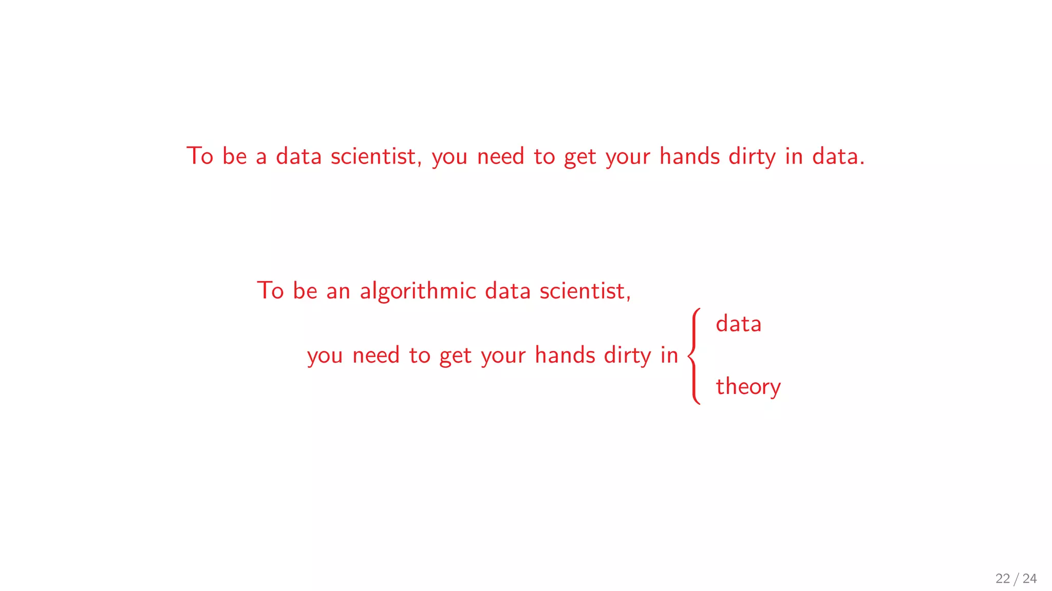
To be a data scientist, you need to get your hands dirty in data. To be an algorithmic data scientist, you need to get your hands dirty in    data theory 22 / 24

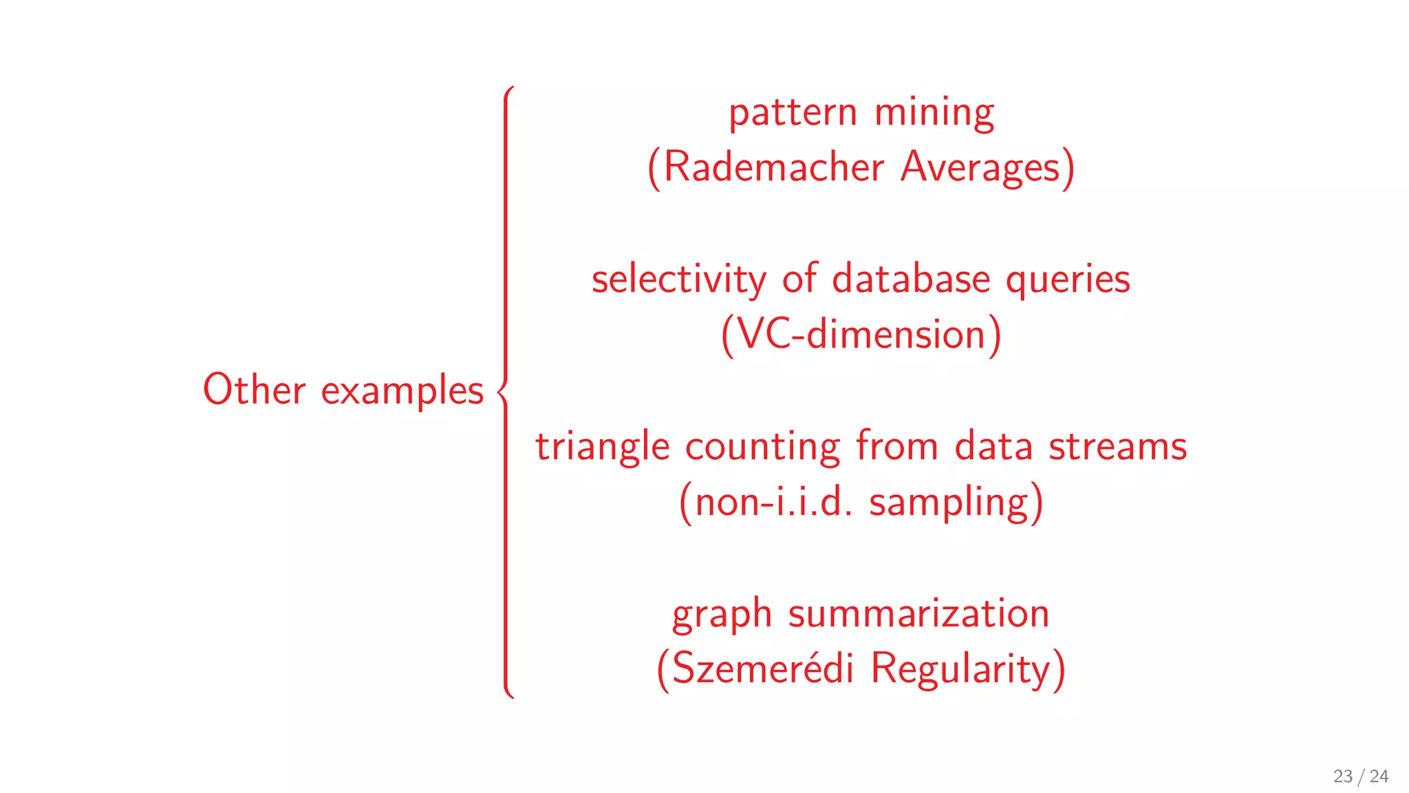
Other examples    pattern mining (Rademacher Averages) selectivity of database queries (VC-dimension) triangle counting from data streams (non-i.i.d. sampling) graph summarization (Szemerédi Regularity) 23 / 24

1) Embrace data science 2) Combine theory and practice 24 / 24

1) Embrace data science 2) Combine theory and practice Thank you! EML: matteo@twosigma.com TWTR: @teorionda WWW: http://matteo.rionda.to 24 / 24

This document is being distributed for informational and educational purposes only and is not an offer to sell or the solicitation of an offer to buy any securities or other instruments. The information contained herein is not intended to provide, and should not be relied upon for investment advice. The views expressed herein are not necessarily the views of Two Sigma Investments, LP or any of its affiliates (collectively, “Two Sigma”). Such views reflect significant assumptions and subjective of the author(s) of the document and are subject to change without notice. The document may employ data derived from third-party sources. No representation is made as to the accuracy of such information and the use of such information in no way implies an endorsement of the source of such information or its validity. The copyrights and/or trademarks in some of the images, logos or other material used herein may be owned by entities other than Two Sigma. If so, such copyrights and/or trademarks are most likely owned by the entity that created the material and are used purely for identification and comment as fair use under international copyright and/or trademark laws. Use of such image, copyright or trademark does not imply any association with such organization (or endorsement of such organization) by Two Sigma, nor vice versa.

Algorithmic Data Science = Theory + Practice

More Related Content

What's hot

Similar to Algorithmic Data Science = Theory + Practice

More from Two Sigma

Recently uploaded

Algorithmic Data Science = Theory + Practice