2. Array in Data Structure

Data Structures 2  An array is a list of a finite number of homogenous (similar data) elements.  This means that an array can store either all integers, all floating point numbers, all characters (string) or any other complex data type but all of same type. Arrays

• There are some important points : – Arrays are always stored in successive memory locations. – An array can store multiple values which can be referenced by a single name. – Array name is actually a pointer to the first location of the memory block allocated to the name of the array – An array either be an integer, character or floating data type can be initialized only during declaration time, and not afterwards – There is no bound checking concept for arrays in C. Data Structures 3

• Elements of an array A may be denoted by the subscript notation A1, A2, …………… An Or A[1], A[2],………..A[n] • The number n of elements is called the length or size of the array. • The number n in A[n] is called a subscript / index and A[n] is called a subscript variable. Data Structures 4

• Length / Size of array = UB – LB + 1 • Where UB is the largest index, called the upper bound, and LB is the smallest index, called the lower bound of the array Length = UB where LB =1 Data Structures 5

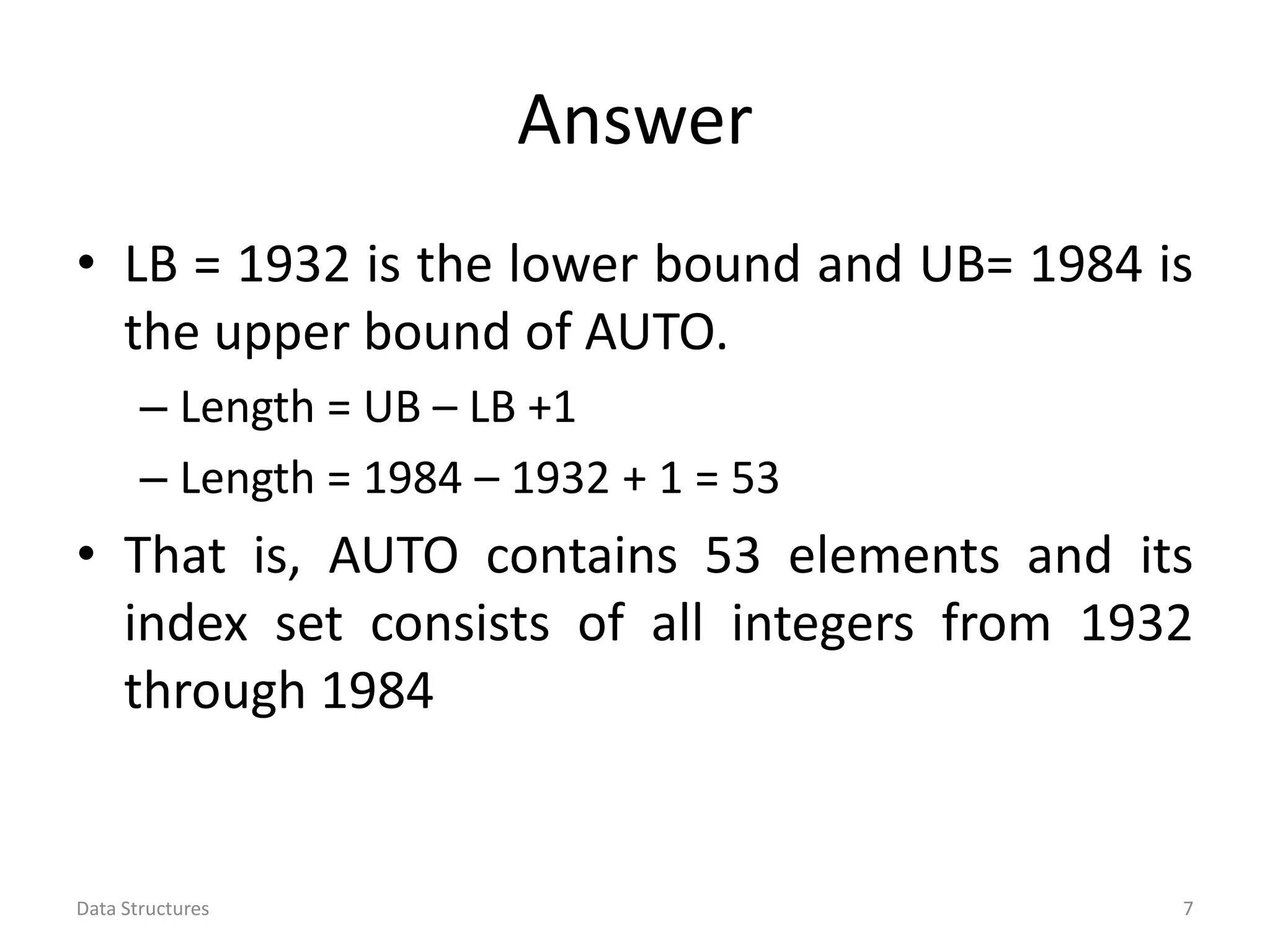
Example • An automobile company uses an array AUTO to record the number of automobiles sold each year from 1932 through 1984. Rather than beginning the index set with 1, it is more useful to begin the index set with 1932 so that • AUTO[K] = number of automobiles sold in the year K. Data Structures 6

Answer • LB = 1932 is the lower bound and UB= 1984 is the upper bound of AUTO. – Length = UB – LB +1 – Length = 1984 – 1932 + 1 = 53 • That is, AUTO contains 53 elements and its index set consists of all integers from 1932 through 1984 Data Structures 7

One Dimensional Arrays • A one dimensional array is one in which only one subscript specification is needed to specify a particular element of the array. • One dimensional array can be declared as : Data_type var_name [expression]; • Where data_type is the type of elements to be stored in the array. • Var_name specifies the name of array, • Expression or subscript specifies the number of values to be stored in the array. Data Structures 8

• Example : • Int num[5] • The array will store five integer values, its name is num • num[0]=22, num[1] = 1, num[2]=30, num[3]=9, num[4]=3 num 0 1 2 3 4 Data Structures 9 22 1 30 9 3

• The size of array can be determine as : • Size = UB – LB +1 • For array num size will be : • UB = 4 • LB = 0 • Size = 4 – 0 +1 = 5 • Size of array in bytes (i.e. amount of memory array occupies) Data Structures 10

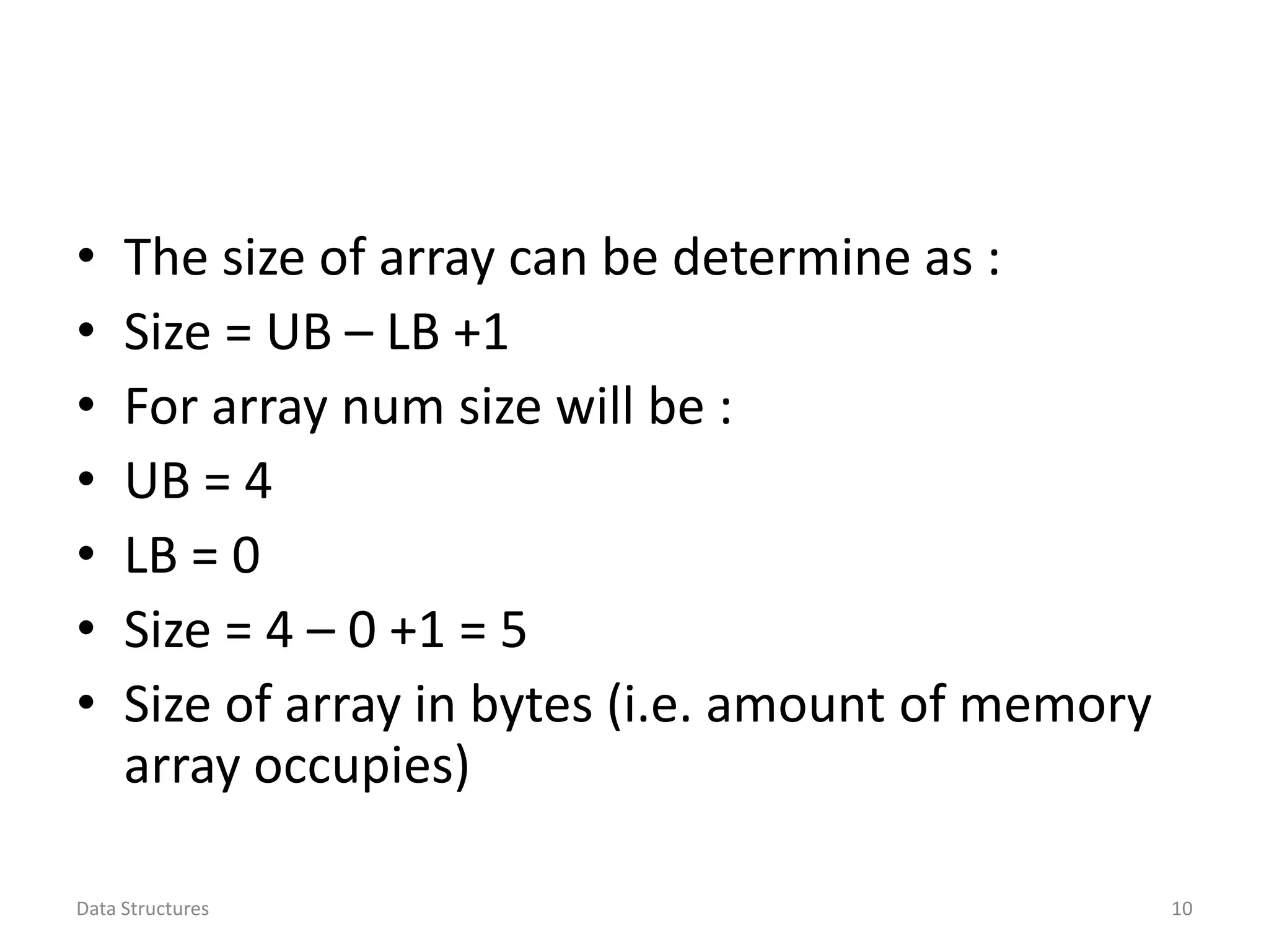
• Size in bytes = size of array x size of base type • E.g. if we have array int num [5]; • Then size in bytes = 5 x 2 = 10 bytes • Similarly, if we have array float num[5]; • Then size in bytes = 5 x 4 = 20 bytes Data Structures 11

Data Structures 12 Initializing Array • int n[ 5 ] = { 1, 2, 3, 4, 5 }; – If not enough initializers, rightmost elements become 0 –int n[ 5 ] = { 0 }  All elements 0 – If too many initializers, a syntax error occurs – C arrays have no bounds checking!! • If size omitted, initializers determine it  int n[ ] = { 1, 2, 3, 4, 5 }; – 5 initializers, therefore 5 element array

Data Structures 13 Addressing of element in 1-D Array • Let A be a linear array stored in successive memory cells. LOC(A[K]) = address of the element A[K] of the array A 1000 1001 1002 1003 • To calculate the address of any element of A formula is:: LOC(A[K])= Base (A) + w (K-lower bound) • Base (A) =Address of the first element of A • w =number of words per memory cell for the array • K =any index of A

Example • Consider the array AUTO in which records the number of automobiles sold each year from 1932 through 1984. Suppose AUTO appears in memory as pictured. That is Base(AUTO) = 200 and w = 4 words per memory cell for AUTO Then • LOC(AUTO[1932]) = 200, • LOC(AUTO[1933])=204, • LOC(AUTO[1934])=208,….. • The address of the array element for the year K=1965 can be obtained by using formula. Data Structures 14

Answer • LOC(AUTO[1965]) = Base(AUTO) + w (1965 – lower bound) • LOC(AUTO[1965])= 200 + 4 (1965 – 1932) • LOC(AUTO[1965]) = 332 Data Structures 15

Data Structures 16 Implementation of linear array • Let LA be a linear array and stored in computer memory .Now we want to count the no. of elements of LA or print the contents of each element of LA, this is done by traversing LA • Also we want to insert an item in the linear array, done by Insert operation • Also we want to delete an item in the linear array, done by Delete operation

Data Structures 17 Algo. For Traversing in linear array • LA is a linear array with UB upper bound and LB lower bound for traversing we apply PROCESS to each element of LA Steps are: 1.Set k=LB 2.Repeat step 3 and 4 while k<=UB 3.Apply PROCESS to LA [k] 4.k=k+1 5.exit

Data Structures 18 Inserting an element in array • INSERT (LA, N, k, ITEM) Here LA is a Linear array with N elements and K is a positive integer. This algorithm inserts an element ITEM into the Kth position in LA. Steps are: 1.Set j=N 2. Repeats step 3 and 4 while j>=k 3.Set LA[j+1]=LA[j] 4.Set j=j-1 5.Set LA[k]=ITEM 6.Set N=N+1 7.Exit

Data Structures 19 Delete an element in array • DELETE (LA, N, k, ITEM) Here LA is a Linear array with N elements and K is a positive integer. This algorithm deletes the Kth element from LA. Steps are: 1.Set ITEM = LA[k] 2. Repeat for j = k to N-1 Set LA[j] = LA[j+1] 3.Set N=N-1 4.Exit

Disadvantages of linear Array • The number of elements, which is to be stored in an array must be known first. • These are static structures. Static in the sense that memory is allocated at compilation time. • When an array is declared, memory is allocated to it. If memory is not filled completely, the vacant place occupies memory. Data Structures 20

• The elements of the arrays are stored in consecutive locations, the insertion and deletion into the array are time consuming. Because to insert/delete an item require moving elements down to create a space for new element or moving elements up to occupy the space by the deleted element. Data Structures 21

Data Structures 22 Two-Dimensional Array (Table) Col 0 Col 1 Col 2 Col 3 Col 4 Row 0 a[0][0] a[0][1] a[0][2] a[0][3] a[0][4] Row 1 a[1][0] a[1][1] a[1][2] a[1][3] a[1][4] Row 2 a[2][0] a[2][1] a[2][2] a[2][3] a[2][4] ►short a[3][5]; // a table with 3 rows,5 columns ►The first dimension denotes the row-index, which starts with 0. ►The second dimension denotes the column- index, which also starts with 0.

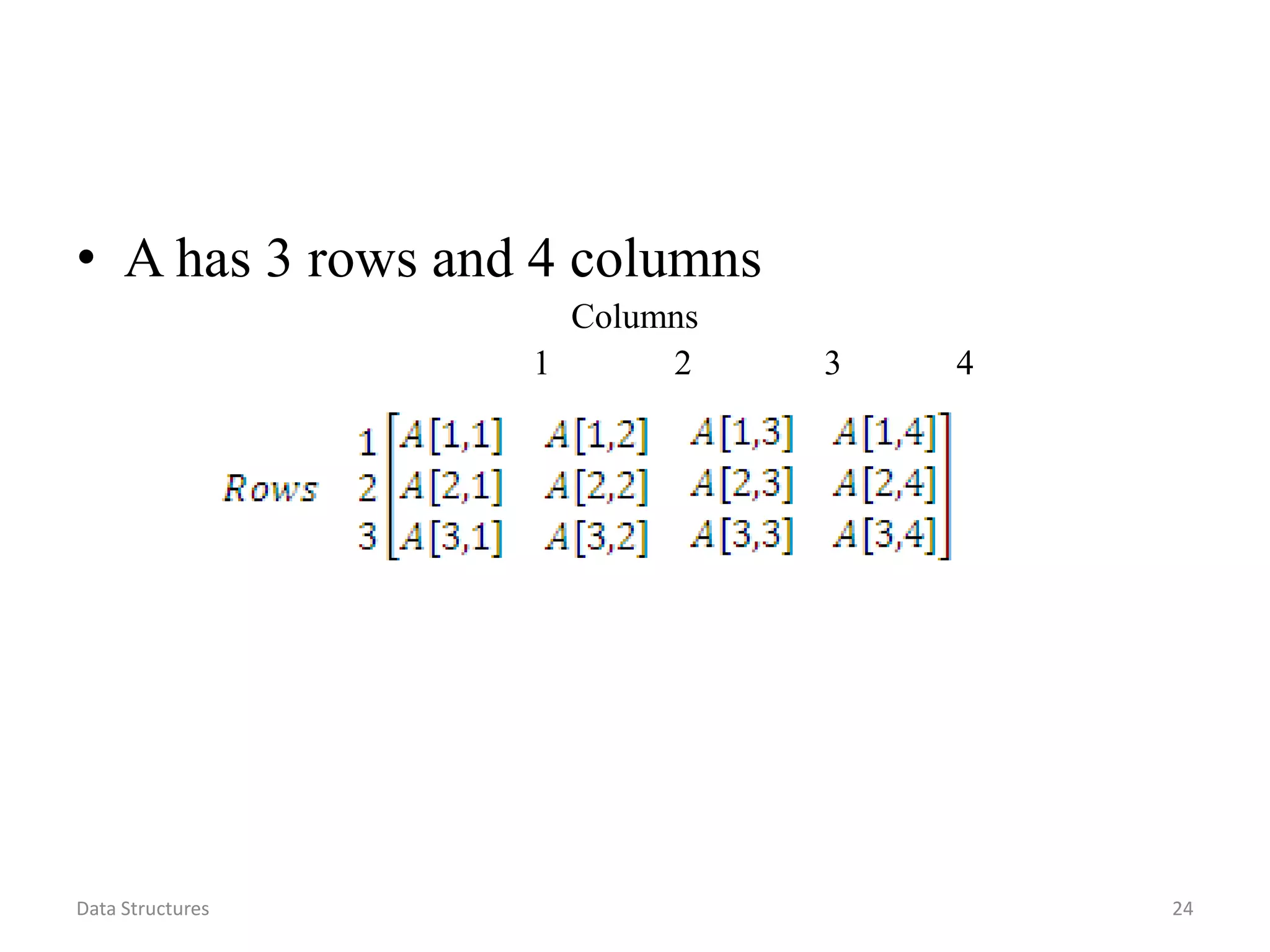
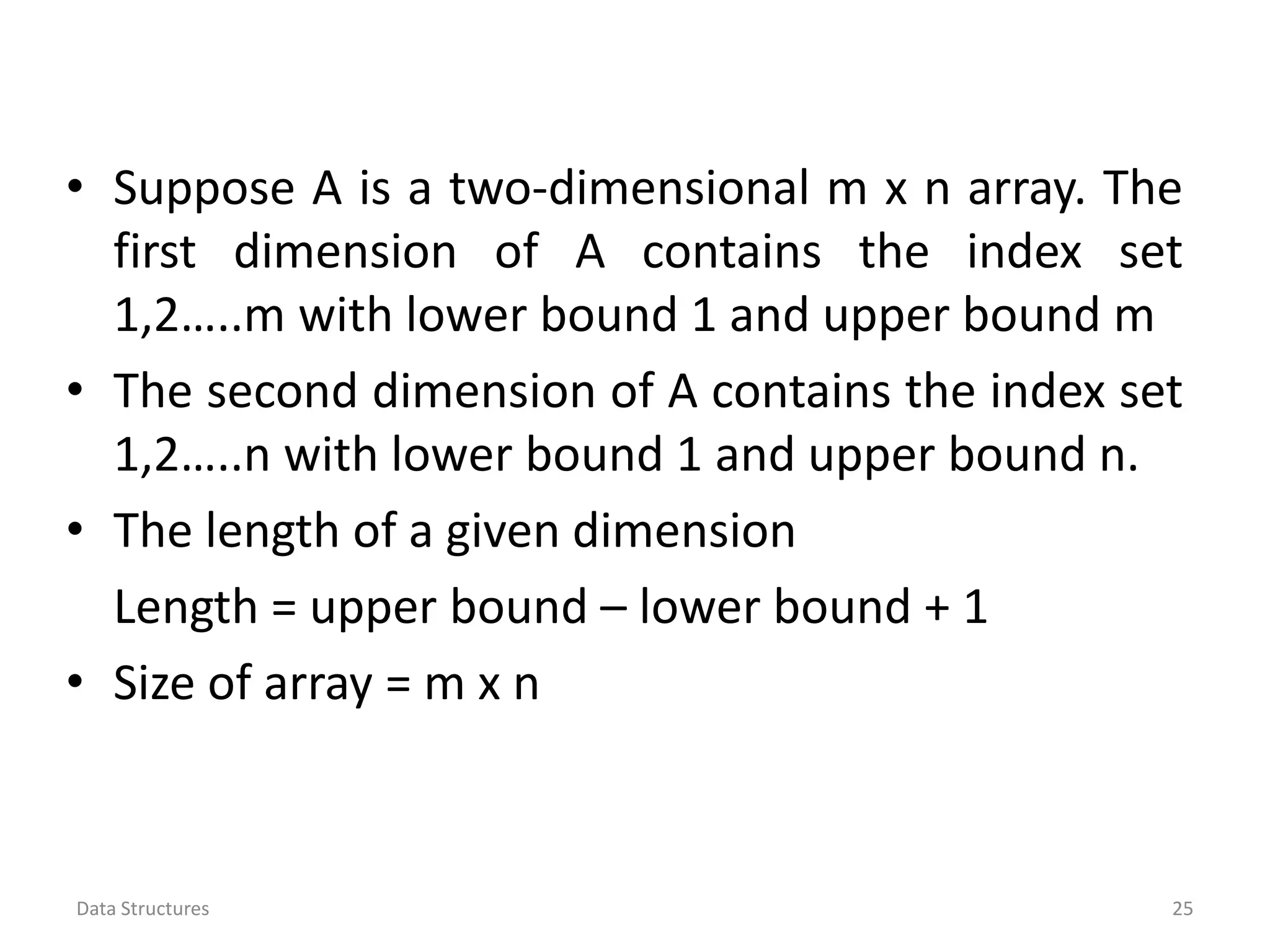
Data Structures 23 Two-Dimensional Array • A two dimensional array A is a collection of m * n elements and each element is specified by pair of integers (such as J, K) called subscripts 1<=J<= m AND 1<=K<=n • Element of A with first subscript j and second subscript k will denoted by AJ,K or A[J,K] • Two-dimensional arrays are called matrices in mathematics and tables in business applications. • The element A[J,K] appears in row J and column K • A row is a horizontal list of elements and a column is a vertical list of elements.

• A has 3 rows and 4 columns Columns 1 2 3 4 Data Structures 24

• Suppose A is a two-dimensional m x n array. The first dimension of A contains the index set 1,2…..m with lower bound 1 and upper bound m • The second dimension of A contains the index set 1,2…..n with lower bound 1 and upper bound n. • The length of a given dimension Length = upper bound – lower bound + 1 • Size of array = m x n Data Structures 25

Data Structures 26 EXAMPLE • Let A be a 2D array such that • A(2:5,-3:1) • Here index set of dimensions 2,3,4,5 and -3,- 2,-1,0,1 • Length of first dimension is 5-2+1=4 • Length of second dimension is 1-(-3)+1=5 • Size of A=4*5=20

Representation of 2D array in memory • There are two ways of representing 2D array • Row major array • Column major array • Row major array : The elements are stored row by row i.e. n elements of the first row stored in first n locations, elements of the second row stored in next n locations and so on. • Column major array : The elements are stored column by column i.e. m elements of the first column stored in first m locations, elements of the second column stored in next m locations and so on. Data Structures 27

Data Structures 28 Representation of 2D array in memory (1,1) (1,2) (1,3) (2,1) (2,2) (2,3) subscriptsA Row 1 Row2 Row-major order

Data Structures 29 Representation of 2D array in memory (1,1) (2,1) (3,1) (2,1) (2,2) (2,3) subscriptsA column 1 column2 Column major order

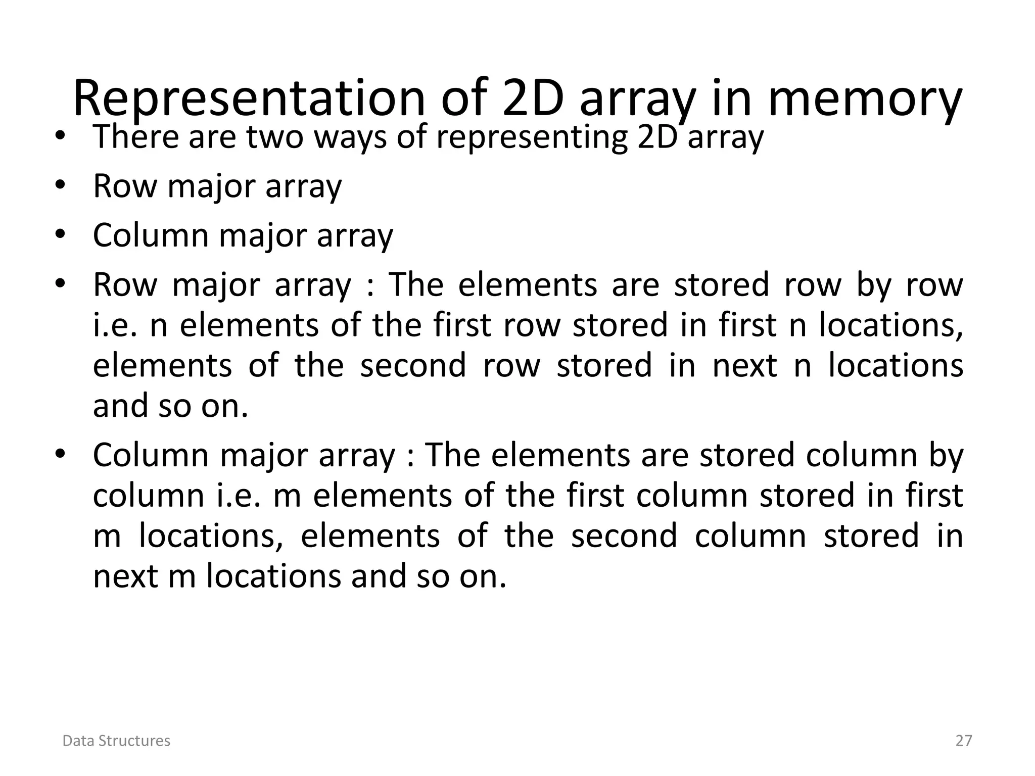
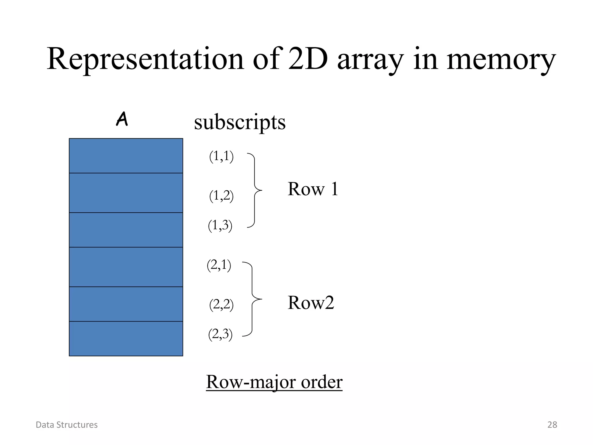
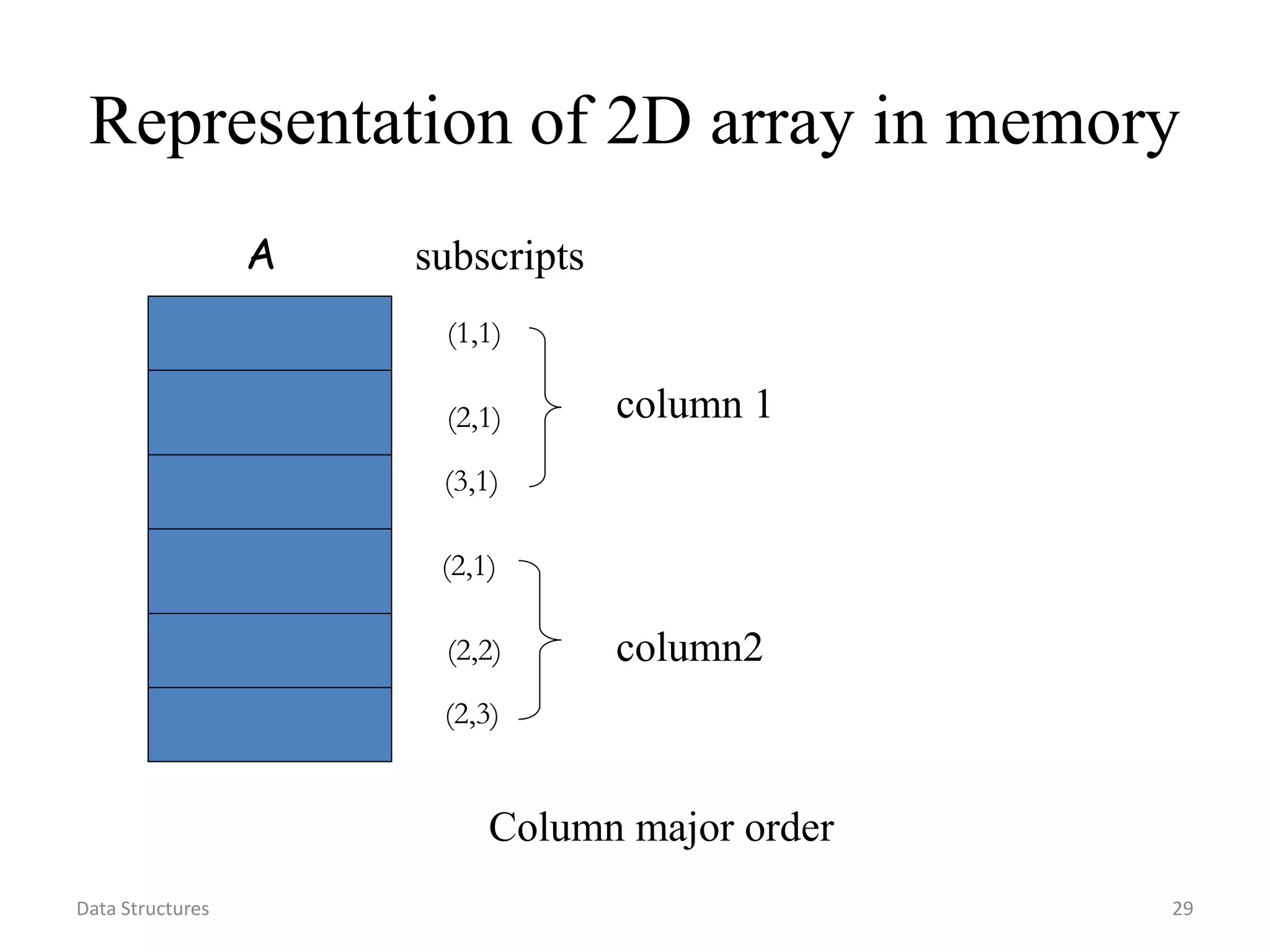
Data Structures 30 Address calculation in 2D array • Let a 2D array A of m*n size, to compute the LOC (A[j,k]) using the formula LOC (A[j,k])=Base(A)+w[(N(j-1)+(k-1)] (row major order) Where Base(A) = address of 1st element of A, w = words per memory cell and N = total no. of columns in array LOC (A[j,k])=Base(A)+w[(M(k-1)+(j-1)] (column major order) Where Base(A) = address of 1st element of A, w = words per memory cell and M = total no. of rows in array

Example • Consider the 25 x 4 matrix array SCORE. Suppose Base(SCORE) = 200 & w= 4. Calculate the address of SCORE = [12,3] i.e. the 12th row and 3 column using row major order and column major order. Data Structures 31

Answer • M = 25, • N = 4 • J = 12 • K = 3 • W = 4 • Base (SCORE) =200 Data Structures 32

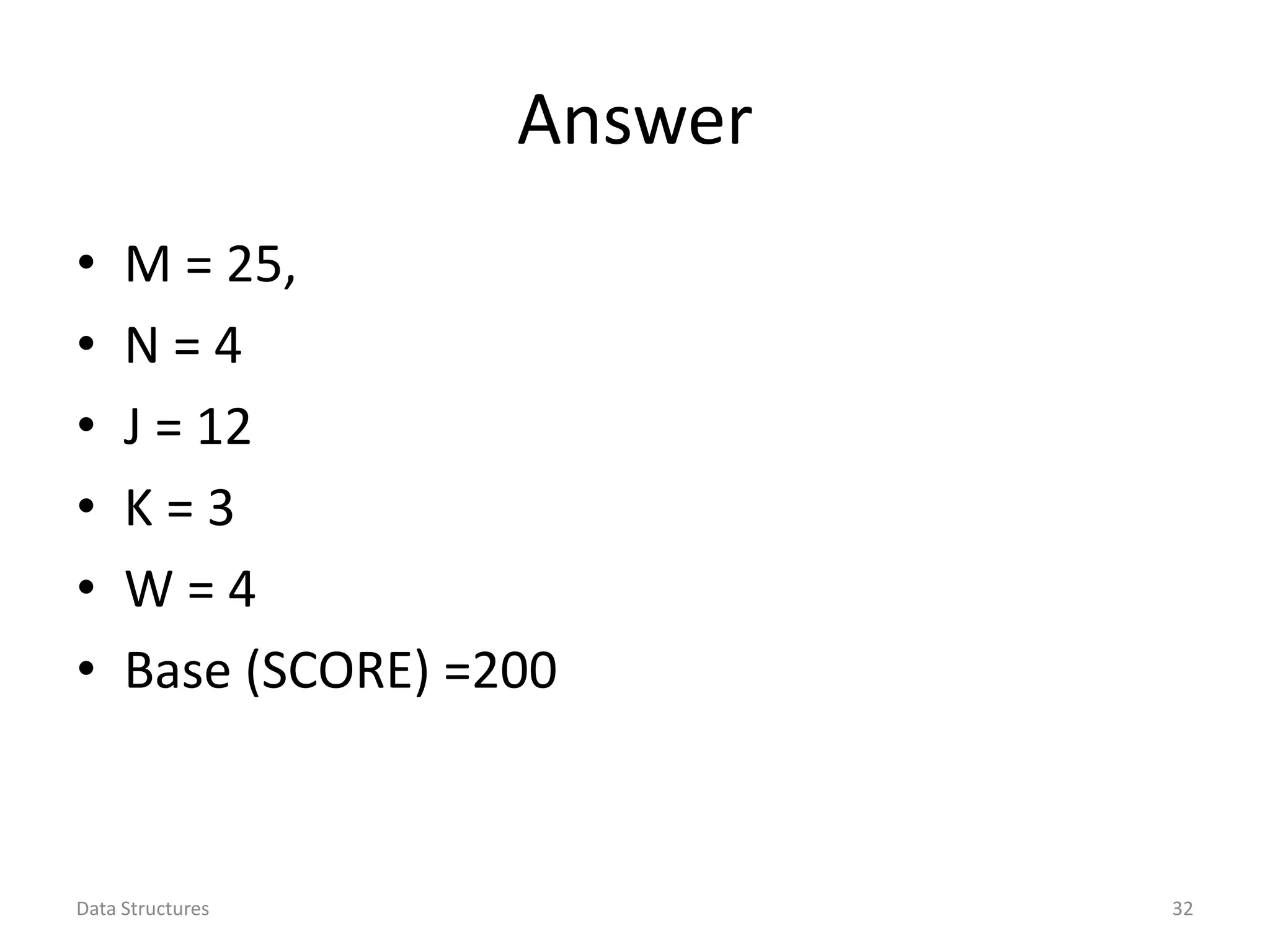
Using Row-major order • LOC (SCORE[12,3]) = Base (SCORE) + w [N(J-1) + (K-1)] = 200 + 4 [4(12-1) + (3-1)] = 200 + 4 [4(11) + 2)] = 200 + 4 [44 +2] = 200 + 4 [46] = 200 + 184 = 384 Data Structures 33

Using Column Major Order • LOC (SCORE[12,3]) = Base (SCORE) + w [M(K-1) + (J-1)] = 200 + 4 [25(3-1) + (12-1)] = 200 + 4 [25(2) + 11)] = 200 + 4 [50 +11] = 200 + 4 [61] = 200 + 244 = 444 Data Structures 34

Multidimensional Array • When array can be extended to any number of dimensions. E.g. 3D array may be defined as : • int a[2][4][3] • Multidimensional array also called arrays of arrays • Suppose C is a 3D 2 x 4 x 3 array. Then B contains 2 x 4 x 3 = 24 elements. These elements appear in 3 layer called pages, column and row. Data Structures 35

2. Array in Data Structure

More Related Content

What's hot

Similar to 2. Array in Data Structure

More from Mandeep Singh

Recently uploaded

In this document

2. Array in Data Structure