NumPy - Logistic Distribution

---

---

What is a Logistic Distribution?

The Logistic Distribution is a continuous probability distribution used to model growth and logistic regression.

It is defined by two parameters: the location parameter (mean) and the scale parameter s. The distribution is similar to the normal distribution but has heavier tails, meaning it has a higher probability of extreme values.

Example: The logistic distribution can describe population growth where the rate of increase is proportional to both the amount present and the amount of growth remaining.

The probability density function (PDF) of the logistic distribution is defined as −

 f(x; , s) = (e-(x-)/s) / (s * (1 + e-(x-)/s)2) 

Where,

• : Location parameter (mean).
• s: Scale parameter (related to the standard deviation).
• x: Value of the random variable.
• e: Euler's number (approximately 2.71828).

Generating Logistic Distributions with NumPy

NumPy provides the numpy.random.logistic() function to generate samples from a logistic distribution. You can specify the location parameter , the scale parameter s, and the size of the generated samples.

Example

In this example, we generate 10 random samples from a logistic distribution with a location parameter =0 and a scale parameter s=1 −

 import numpy as np # Generate 10 random samples from a logistic distribution with =0 and s=1 samples = np.random.logistic(loc=0, scale=1, size=10) print("Random samples from logistic distribution:", samples) 

Following is the output obtained −

 Random samples from logistic distribution: [-1.6473898 1.18698013 -0.24048488 -1.05235482 3.11858778 -1.40235809 0.8399973 -1.46670621 -3.14359949 -0.80023521] 

Visualizing Logistic Distributions

Visualizing logistic distributions helps to understand their properties better. We can use libraries such as Matplotlib to create histograms that display the distribution of generated samples.

Example

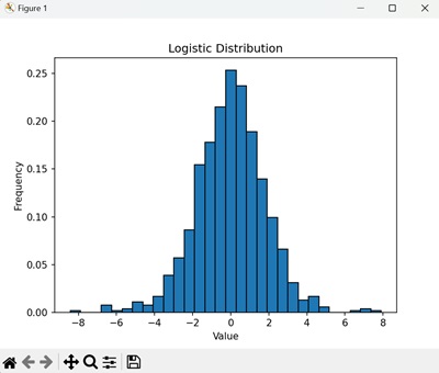
In the following example, we are first generating 1000 random samples logistic distribution with =0 and s=1. We are then creating a histogram to visualize this distribution −

 import numpy as np import matplotlib.pyplot as plt # Generate 1000 random samples from a logistic distribution with =0 and s=1 samples = np.random.logistic(loc=0, scale=1, size=1000) # Create a histogram to visualize the distribution plt.hist(samples, bins=30, edgecolor='black', density=True) plt.title('Logistic Distribution') plt.xlabel('Value') plt.ylabel('Frequency') plt.show() 

The histogram shows the frequency of the values in the logistic distribution. The bars represent the probability of each possible outcome, forming the characteristic S-shape of the logistic distribution −

Applications of Logistic Distributions

Logistic distributions are used in various fields to model data with extreme values. Here are a few practical applications −

• Machine Learning: Modeling binary outcomes in logistic regression.
• Economics: Modeling growth and distribution of income and wealth.
• Statistics: Analyzing and predicting outcomes with a logistic model.

Generating Cumulative Logistic Distributions

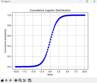
Sometimes, we are interested in the cumulative distribution function (CDF) of a logistic distribution, which gives the probability of getting up to and including x events in the interval.

NumPy does not have a built-in function for the CDF of a logistic distribution, but we can calculate it using a loop and the scipy.stats.logistic.cdf() function from the SciPy library.

Example

Following is an example to generate cumulative logistic distribution in NumPy −

 import numpy as np import matplotlib.pyplot as plt from scipy.stats import logistic # Define the location and scale parameters loc = 0 scale = 1 # Generate the cumulative distribution function (CDF) values x = np.linspace(-10, 10, 100) cdf = logistic.cdf(x, loc=loc, scale=scale) # Plot the CDF plt.plot(x, cdf, marker='o', linestyle='-', color='b') plt.title('Cumulative Logistic Distribution') plt.xlabel('Value') plt.ylabel('Cumulative probability') plt.grid(True) plt.show() 

The plot shows the cumulative probability of getting up to and including each value in the logistic trials. The CDF is a smooth curve that increases to 1 as the value increases −

Properties of Logistic Distributions

Logistic distributions have several key properties, such as −

• Location Parameter (): The location parameter is the mean of the distribution.
• Scale Parameter (s): The scale parameter is related to the standard deviation of the distribution.
• Mean and Variance: The mean of a logistic distribution is , and the variance is (s²²/3).
• Skewness: The distribution is symmetric around the mean, with heavier tails than a normal distribution.

Using Logistic Distribution for Hypothesis Testing

Logistic distributions are often used in hypothesis testing, particularly in tests for binary outcomes.

One common test is logistic regression, which is used to model the probability of a binary outcome based on one or more predictor variables. Here is an example using the statsmodels library:

Example

In this example, we fit a logistic regression model to binary outcome data. The summary provides information about the coefficients, standard errors, and p-values of the model −

 # Python version 3.11 import numpy as np import statsmodels.api as sm # Example data X = np.array([0, 1, 2, 3, 4, 5]) y = np.array([0, 0, 0, 1, 1, 1]) # Add a constant to the predictor variable X = sm.add_constant(X) # Fit the logistic regression model model = sm.Logit(y, X) result = model.fit(method='lbfgs', maxiter=100, disp=0) # Print the model summary print(result.summary()) 

The output obtained is as shown below −

 Logit Regression Results ============================================================================== Dep. Variable: y No. Observations: 6 Model: Logit Df Residuals: 4 Method: MLE Df Model: 1 Date: Wed, 20 Nov 2024 Pseudo R-squ.: 1.000 Time: 12:29:27 Log-Likelihood: -5.7054e-05 converged: True LL-Null: -4.1589 Covariance Type: nonrobust LLR p-value: 0.003926 ============================================================================== coef std err z P>|z| [0.025 0.975] ------------------------------------------------------------------------------ const -52.2706 668.240 -0.078 0.938 -1361.997 1257.456 x1 20.9332 265.301 0.079 0.937 -499.046 540.913 ============================================================================== Complete Separation: The results show that there iscomplete separation or perfect prediction. In this case the Maximum Likelihood Estimator does not exist and the parameters are not identified. 

Seeding for Reproducibility

To ensure reproducibility, you can set a specific seed before generating logistic distributions. This ensures that the same sequence of random numbers is generated each time you run the code.

Example

In this example, we set the seed to 42 before generating random samples from a logistic distribution. The seed ensures that the same sequence of samples is generated each time the code is run −

 import numpy as np # Set the seed for reproducibility np.random.seed(42) # Generate 10 random samples from a logistic distribution with =0 and s=1 samples = np.random.logistic(loc=0, scale=1, size=10) print("Random samples with seed 42:", samples) 

Following is the output of the above code −

 Random samples with seed 42: [-0.51278827 2.95957976 1.00476265 0.39987857 -1.68815492 -1.68833811-2.78603295 1.86756387 0.41011316 0.88604138]