Graph Theory - Centrality Measures

Centrality Measures

Centrality measures in graph theory are used to determine the importance of nodes in a network. They help to identify that which nodes are influential, well-connected, or play an important role in passing information.

Centrality measures assign a numerical value to each node in a graph based on its importance in the network. The importance of a node can be defined in different ways, such as −

Degree Centrality: Counts how many direct connections a node has.
Closeness Centrality: Measures how close a node is to all other nodes.
Betweenness Centrality: Finds how often a node appears on the shortest paths between other nodes.
Eigenvector Centrality: Determines a node's importance based on how influential its neighbors are.
PageRank: A special type of eigenvector centrality used to rank web pages.

Degree Centrality

Degree centrality is the simplest centrality measure and is calculated based on the number of edges connected to a node.

In undirected graphs, degree centrality is the total number of edges connected to a node.
In directed graphs, it is divided into: In-degree (the number of incoming edges) and Out-degree (the number of outgoing edges).

Following is the formula of degree centrality −

 Degree Centrality = deg(v) / (N - 1)

where,

deg(v) is the degree of node v.
N is the total number of nodes in the graph.

Example

The following code creates an undirected graph with five nodes and five edges, then calculates the degree centrality for each node −

 import networkx as nx G = nx.Graph() G.add_edges_from([(1, 2), (1, 3), (3, 4), (4, 5), (2, 5)]) degree_centrality = nx.degree_centrality(G) print(degree_centrality)

Following is the output obtained −

 {1: 0.5, 2: 0.5, 3: 0.5, 4: 0.5, 5: 0.5}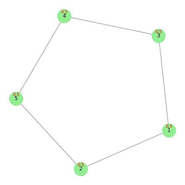

Closeness Centrality

Closeness centrality measures how quickly a node can reach all other nodes in the network. Nodes with high closeness centrality are central in terms of shortest paths.

Following is the formula of closeness centrality −

 Closeness Centrality = (N - 1) / d(v, u)

where,

N is the total number of nodes.
d(v, u) is the shortest path distance between node v and node u.

Example

The following code calculates closeness centrality, and prints the values −

 import networkx as nx # Create an undirected graph G = nx.Graph() G.add_edges_from([(1, 2), (1, 3), (3, 4), (4, 5), (2, 5)]) # Compute closeness centrality closeness_centrality = nx.closeness_centrality(G) # Print closeness centrality values print("Closeness Centrality:", closeness_centrality)

This will produce the following result −

 Closeness Centrality: {1: 0.6666666666666666, 2: 0.6666666666666666, 3: 0.6666666666666666, 4: 0.6666666666666666, 5: 0.6666666666666666}

Betweenness Centrality

Betweenness centrality measures how often a node appears on the shortest paths between other nodes. Nodes with high betweenness centrality act as bridges in the network.

Following is the formula of closeness centrality −

 Betweenness Centrality = ((s, v, t) / (s, t))

where,

(s, t) is the number of shortest paths between nodes s and t.
(s, v, t) is the number of those paths that pass through v.

Example

This code creates an undirected graph with five nodes and five edges, then calculates the betweenness centrality for each node −

 import networkx as nx # Create an undirected graph G = nx.Graph() G.add_edges_from([(1, 2), (1, 3), (3, 4), (4, 5), (2, 5)]) # Compute betweennes centrality betweenness_centrality = nx.betweenness_centrality(G) # Print betweennes centrality values print("Betweenness Centrality:", betweenness_centrality)

The output obtained is as shown below −

 Betweenness Centrality: {1: 0.16666666666666666, 2: 0.16666666666666666, 3: 0.16666666666666666, 4: 0.16666666666666666, 5: 0.16666666666666666}

Eigenvector Centrality

Eigenvector centrality measures the influence of a node based on the importance of its neighbors. Nodes with high eigenvector centrality are connected to other important nodes.

Following is the formula of eigenvector centrality −

 * v = A * v

where,

A is the adjacency matrix of the graph.
v is the eigenvector of the matrix.
is the largest eigenvalue.

Example

The following code calculates the eigenvector centrality for each node in an undirected graph −

 import networkx as nx # Create an undirected graph G = nx.Graph() G.add_edges_from([(1, 2), (1, 3), (3, 4), (4, 5), (2, 5)]) # Compute eigenvector centrality eigenvector_centrality = nx.eigenvector_centrality(G) # Print eigenvector centrality values print("Eigenvector Centrality:", eigenvector_centrality)

The result produced is as follows −

 Eigenvector Centrality: {1: 0.4472135954999579, 2: 0.4472135954999579, 3: 0.4472135954999579, 4: 0.4472135954999579, 5: 0.4472135954999579}

PageRank

PageRank is a variation of eigenvector centrality originally designed for ranking web pages based on their importance.

Following is the formula of pageRank −

 PR(v) = (1 - d) / N + d * (PR(u) / L(u))

where,

d is the damping factor (usually 0.85).
N is the total number of nodes.
PR(u) is the PageRank of node u.
L(u) is the number of outgoing links from u.

Example

This code calculates the PageRank for each node in the given graph. The results are printed as a dictionary −

 import networkx as nx # Create an undirected graph G = nx.Graph() G.add_edges_from([(1, 2), (1, 3), (3, 4), (4, 5), (2, 5)]) # Compute pagerank pagerank = nx.pagerank(G) # Print pagerank values print("PageRank:", pagerank)

We get the output as shown below −

 PageRank: {1: 0.2, 2: 0.2, 3: 0.2, 4: 0.2, 5: 0.2}

Applications of Centrality Measures

Centrality measures are commonly used in various fields −

Social Networks: Finding important users or leaders who influence others.
Biological Networks: Identifying important genes or proteins in living organisms.
Transportation Networks: Finding main locations in road, rail, or air travel systems.
Cybersecurity: Spotting weak points in computer networks that could be attacked.
Recommendation Systems: Ranking products, movies, or other items based on user preferences.

Print Page