Variables , outlier and its detection and Missing values

Topics to be covered 1. Variables and its types 2. Outlier and its detection 3. Missing values Date - 28 Aug 2025

What is a Variable? A variable is something that can change or take different values. ● Example: Your age, height, favorite color, or exam score. ● In statistics, understanding the type of variable is crucial because it determines what analysis we can do.

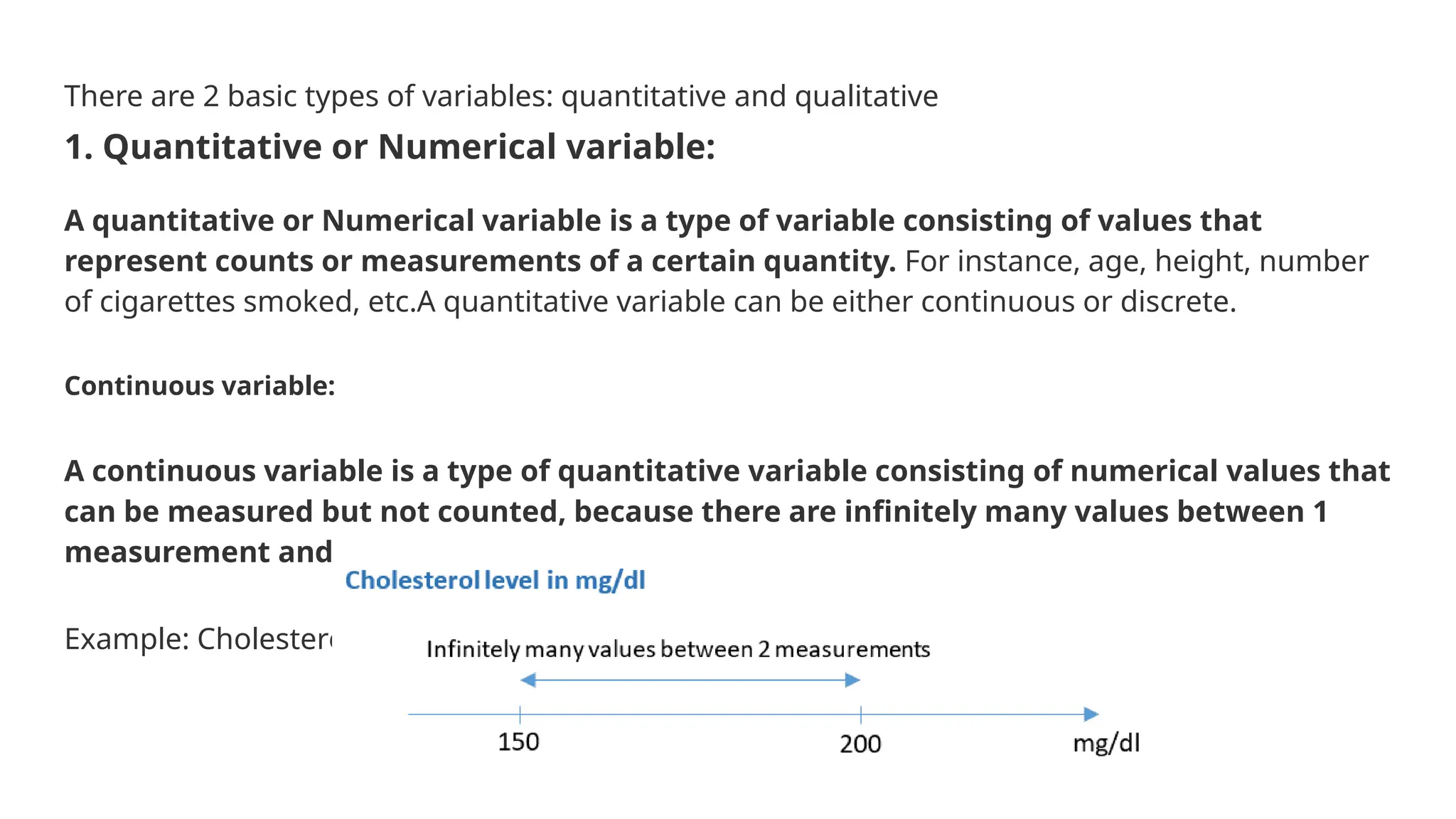
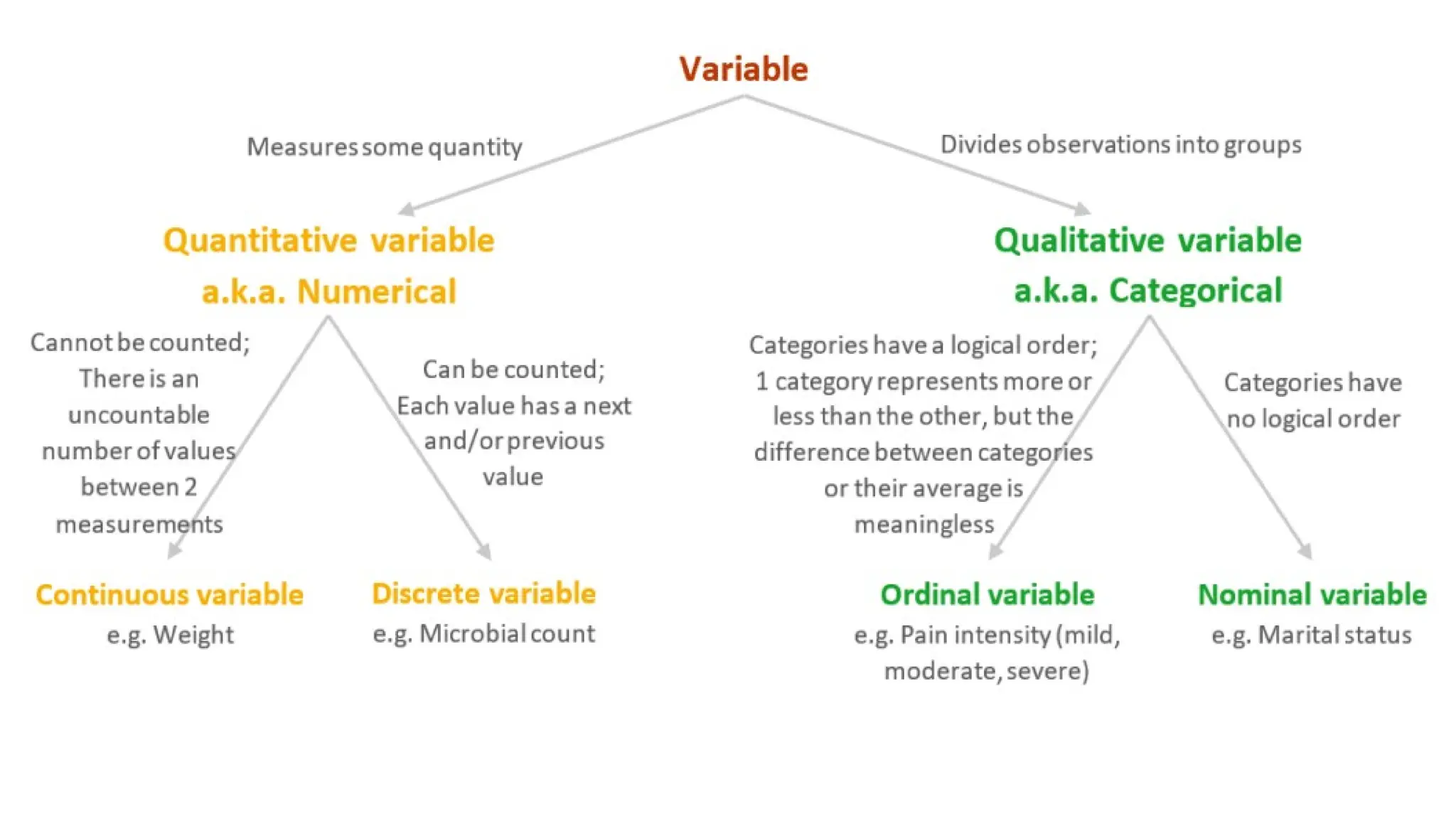
There are 2 basic types of variables: quantitative and qualitative 1. Quantitative or Numerical variable: A quantitative or Numerical variable is a type of variable consisting of values that represent counts or measurements of a certain quantity. For instance, age, height, number of cigarettes smoked, etc.A quantitative variable can be either continuous or discrete. Continuous variable: A continuous variable is a type of quantitative variable consisting of numerical values that can be measured but not counted, because there are infinitely many values between 1 measurement and another. Example: Cholesterol level measured in mg/dl.

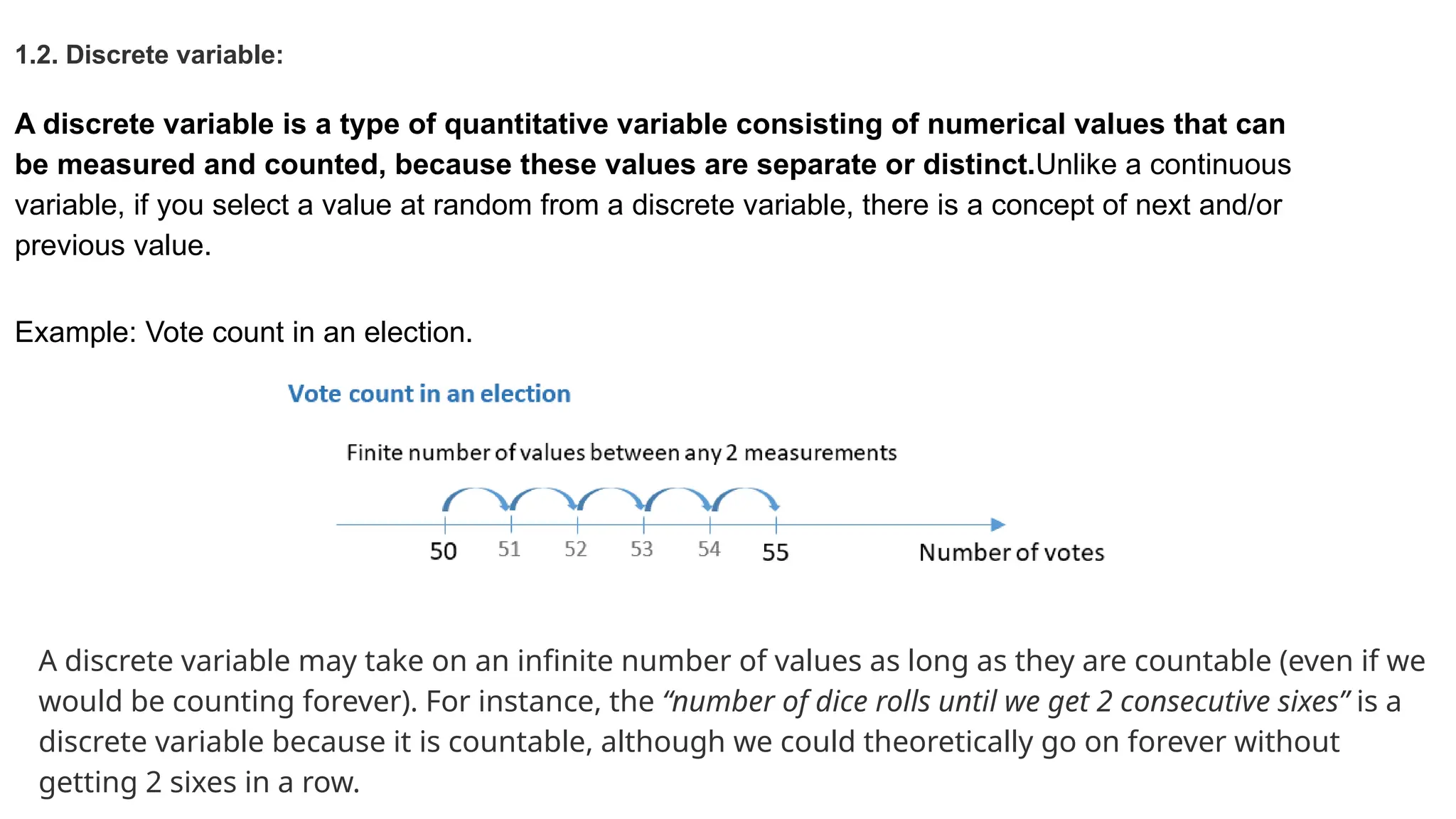
1.2. Discrete variable: A discrete variable is a type of quantitative variable consisting of numerical values that can be measured and counted, because these values are separate or distinct.Unlike a continuous variable, if you select a value at random from a discrete variable, there is a concept of next and/or previous value. Example: Vote count in an election. A discrete variable may take on an infinite number of values as long as they are countable (even if we would be counting forever). For instance, the “number of dice rolls until we get 2 consecutive sixes” is a discrete variable because it is countable, although we could theoretically go on forever without getting 2 sixes in a row.

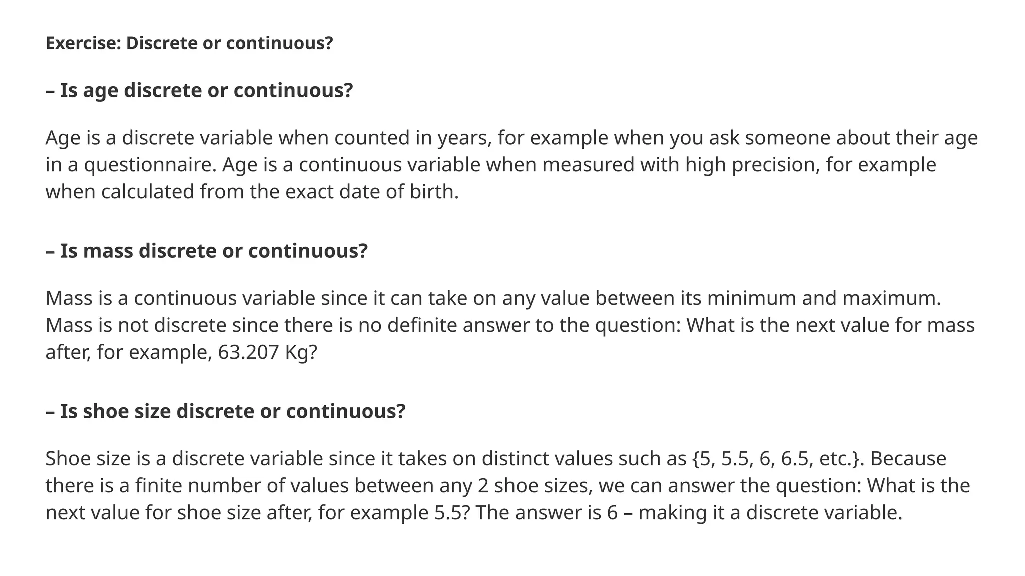
Exercise: Discrete or continuous? – Is age discrete or continuous? Age is a discrete variable when counted in years, for example when you ask someone about their age in a questionnaire. Age is a continuous variable when measured with high precision, for example when calculated from the exact date of birth. – Is mass discrete or continuous? Mass is a continuous variable since it can take on any value between its minimum and maximum. Mass is not discrete since there is no definite answer to the question: What is the next value for mass after, for example, 63.207 Kg? – Is shoe size discrete or continuous? Shoe size is a discrete variable since it takes on distinct values such as {5, 5.5, 6, 6.5, etc.}. Because there is a finite number of values between any 2 shoe sizes, we can answer the question: What is the next value for shoe size after, for example 5.5? The answer is 6 – making it a discrete variable.

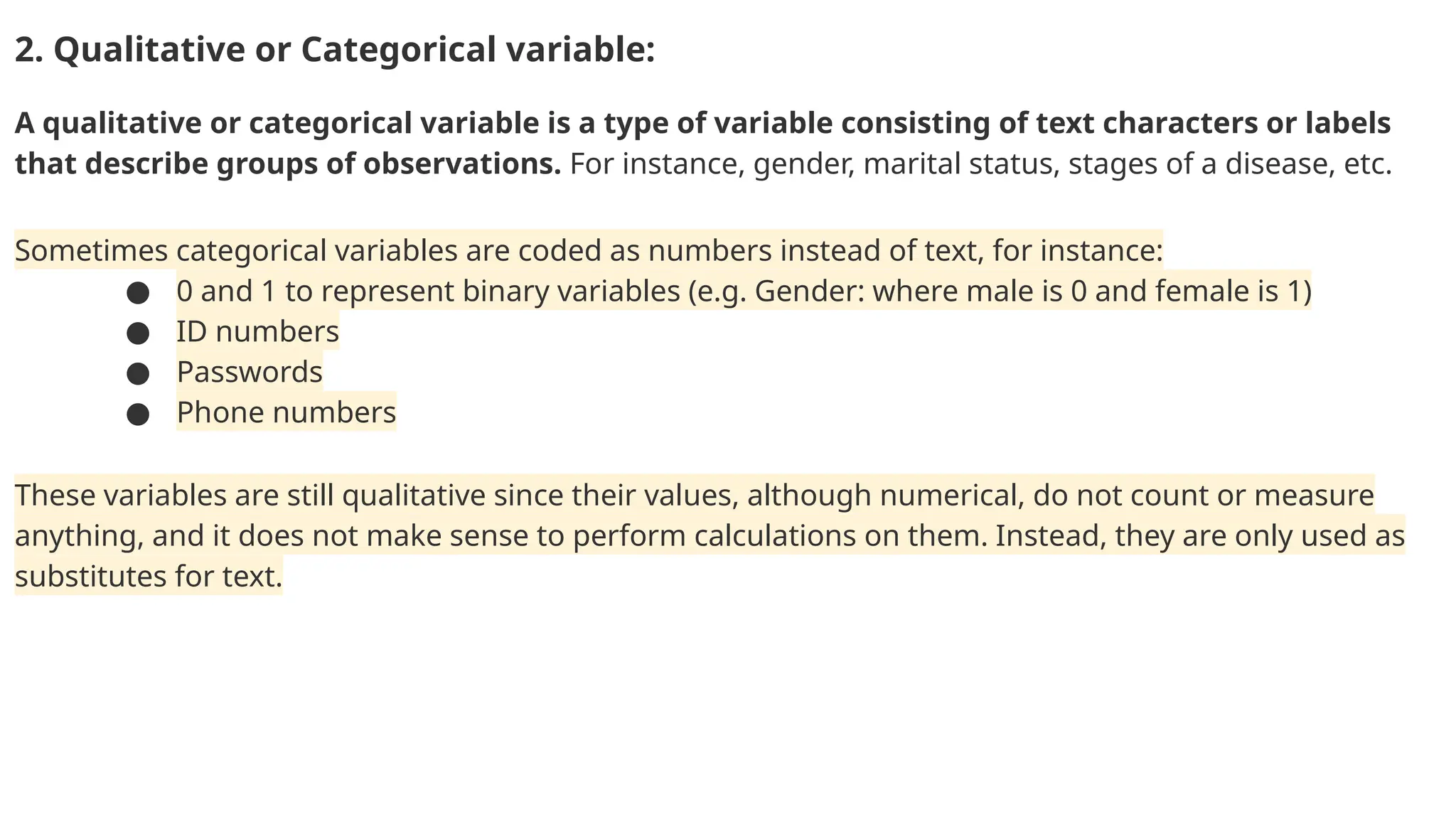
2. Qualitative or Categorical variable: A qualitative or categorical variable is a type of variable consisting of text characters or labels that describe groups of observations. For instance, gender, marital status, stages of a disease, etc. Sometimes categorical variables are coded as numbers instead of text, for instance: ● 0 and 1 to represent binary variables (e.g. Gender: where male is 0 and female is 1) ● ID numbers ● Passwords ● Phone numbers These variables are still qualitative since their values, although numerical, do not count or measure anything, and it does not make sense to perform calculations on them. Instead, they are only used as substitutes for text.

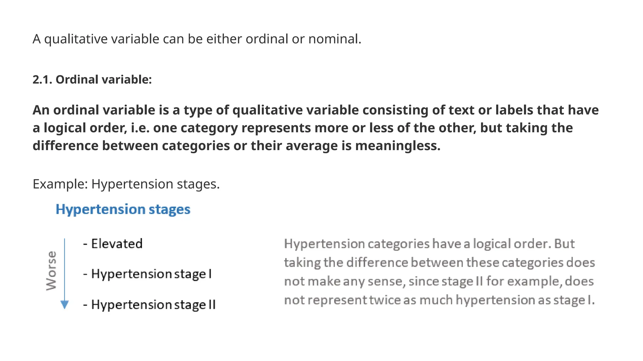
A qualitative variable can be either ordinal or nominal. 2.1. Ordinal variable: An ordinal variable is a type of qualitative variable consisting of text or labels that have a logical order, i.e. one category represents more or less of the other, but taking the difference between categories or their average is meaningless. Example: Hypertension stages.

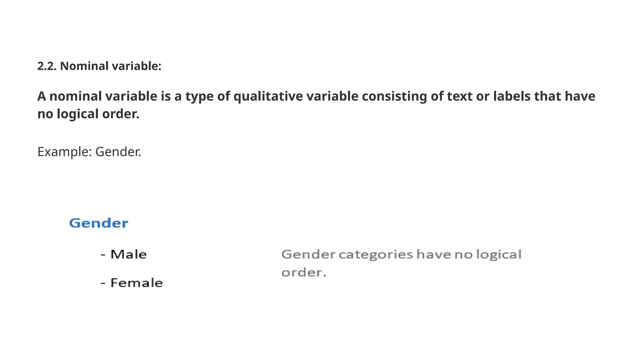
2.2. Nominal variable: A nominal variable is a type of qualitative variable consisting of text or labels that have no logical order. Example: Gender.

Outliers and Outlier Detection Outlier are data point that is essentially a statistical anomaly, a data point that significantly deviates from other observations in a dataset. Outliers can arise due to measurement errors, natural variation, or rare events, and they can have a disproportionate impact on statistical analyses and machine learning models if not appropriately handled. Example: If you have the following dataset of student test scores: [85, 87, 90, 88, 92, 89, 45] The score 45 is an outlier—it’s much lower than the others.

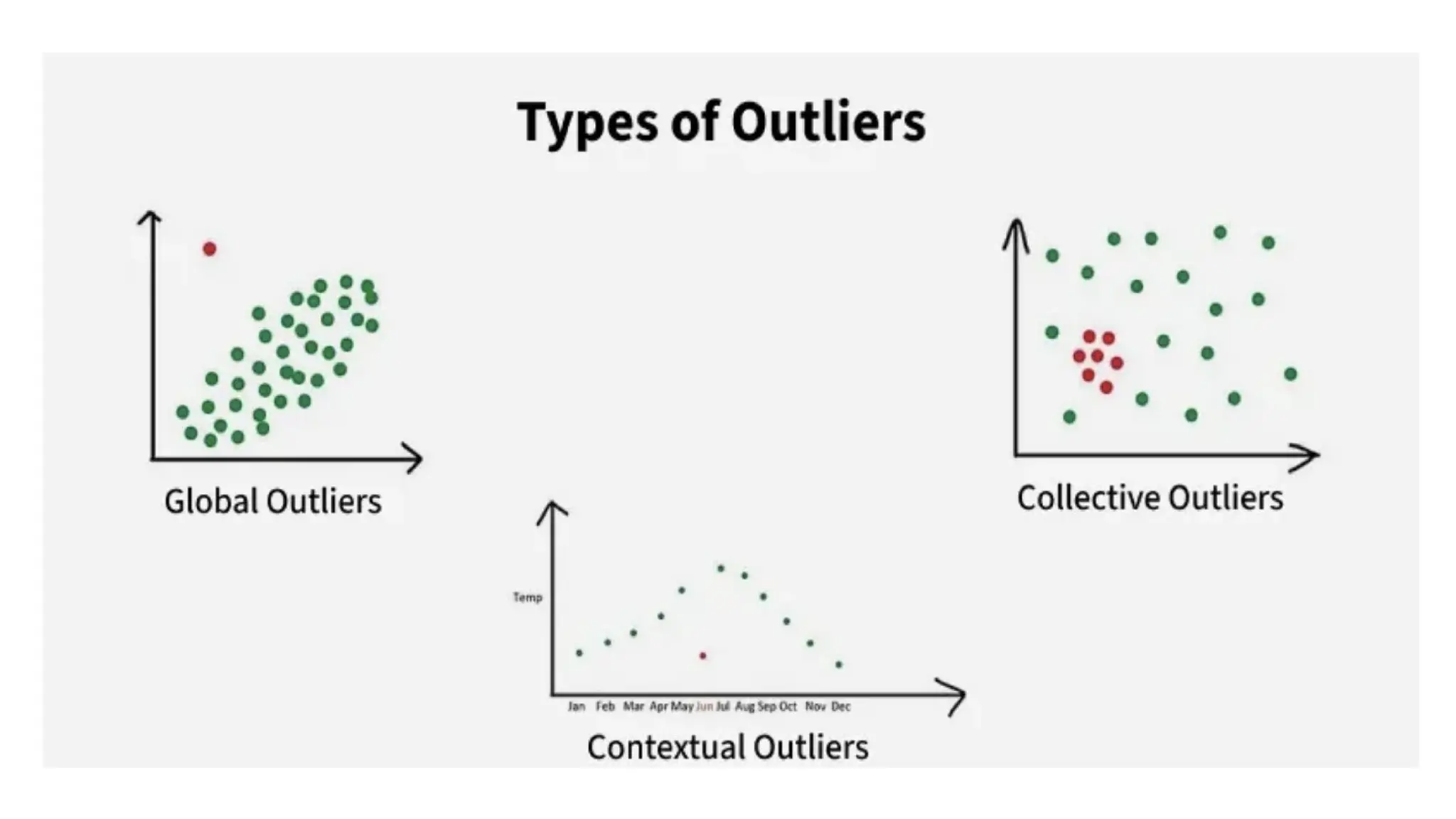
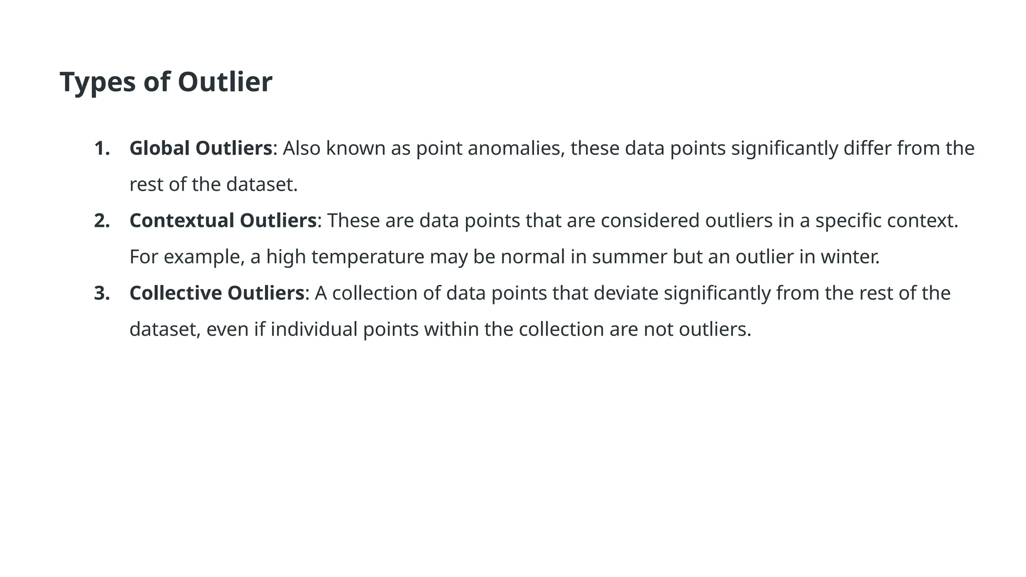
Types of Outlier 1. Global Outliers: Also known as point anomalies, these data points significantly differ from the rest of the dataset. 2. Contextual Outliers: These are data points that are considered outliers in a specific context. For example, a high temperature may be normal in summer but an outlier in winter. 3. Collective Outliers: A collection of data points that deviate significantly from the rest of the dataset, even if individual points within the collection are not outliers.

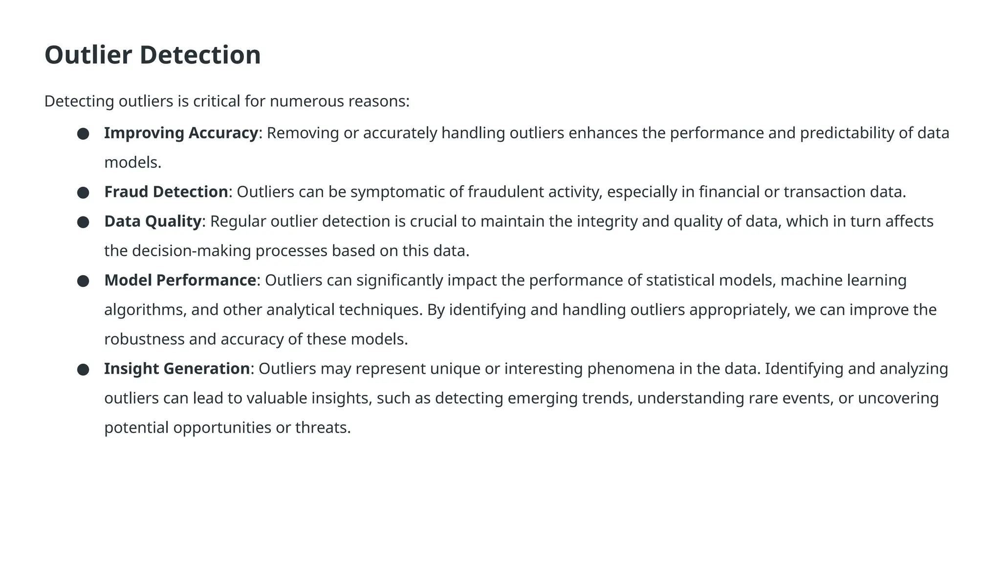
Outlier Detection Detecting outliers is critical for numerous reasons: ● Improving Accuracy: Removing or accurately handling outliers enhances the performance and predictability of data models. ● Fraud Detection: Outliers can be symptomatic of fraudulent activity, especially in financial or transaction data. ● Data Quality: Regular outlier detection is crucial to maintain the integrity and quality of data, which in turn affects the decision-making processes based on this data. ● Model Performance: Outliers can significantly impact the performance of statistical models, machine learning algorithms, and other analytical techniques. By identifying and handling outliers appropriately, we can improve the robustness and accuracy of these models. ● Insight Generation: Outliers may represent unique or interesting phenomena in the data. Identifying and analyzing outliers can lead to valuable insights, such as detecting emerging trends, understanding rare events, or uncovering potential opportunities or threats.

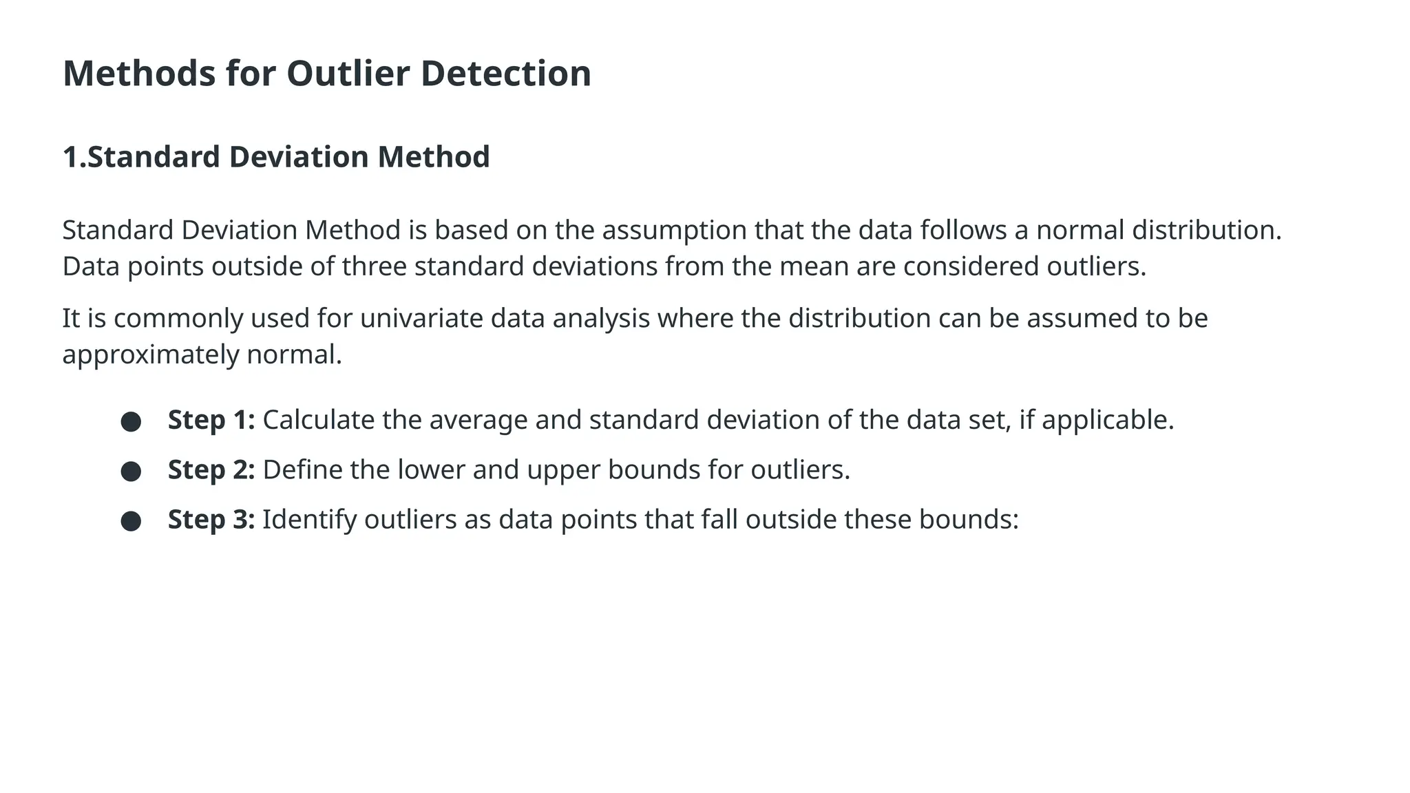
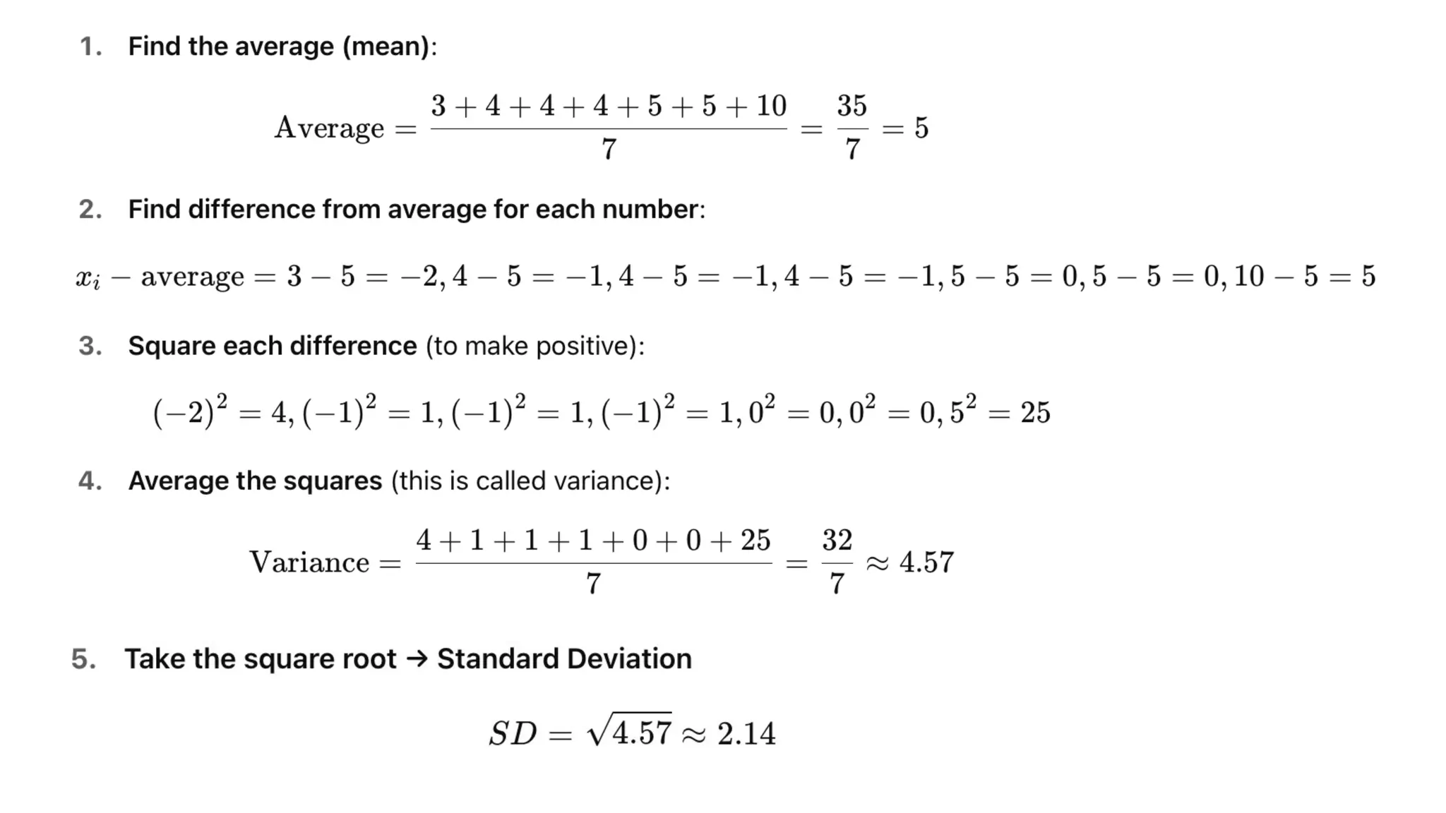
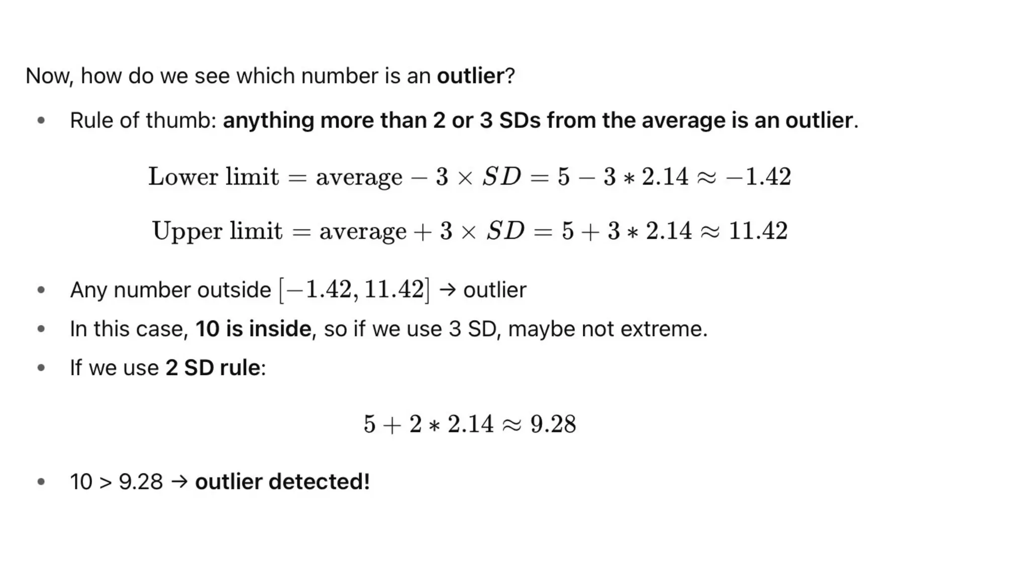
Methods for Outlier Detection 1.Standard Deviation Method Standard Deviation Method is based on the assumption that the data follows a normal distribution. Data points outside of three standard deviations from the mean are considered outliers. It is commonly used for univariate data analysis where the distribution can be assumed to be approximately normal. ● Step 1: Calculate the average and standard deviation of the data set, if applicable. ● Step 2: Define the lower and upper bounds for outliers. ● Step 3: Identify outliers as data points that fall outside these bounds:

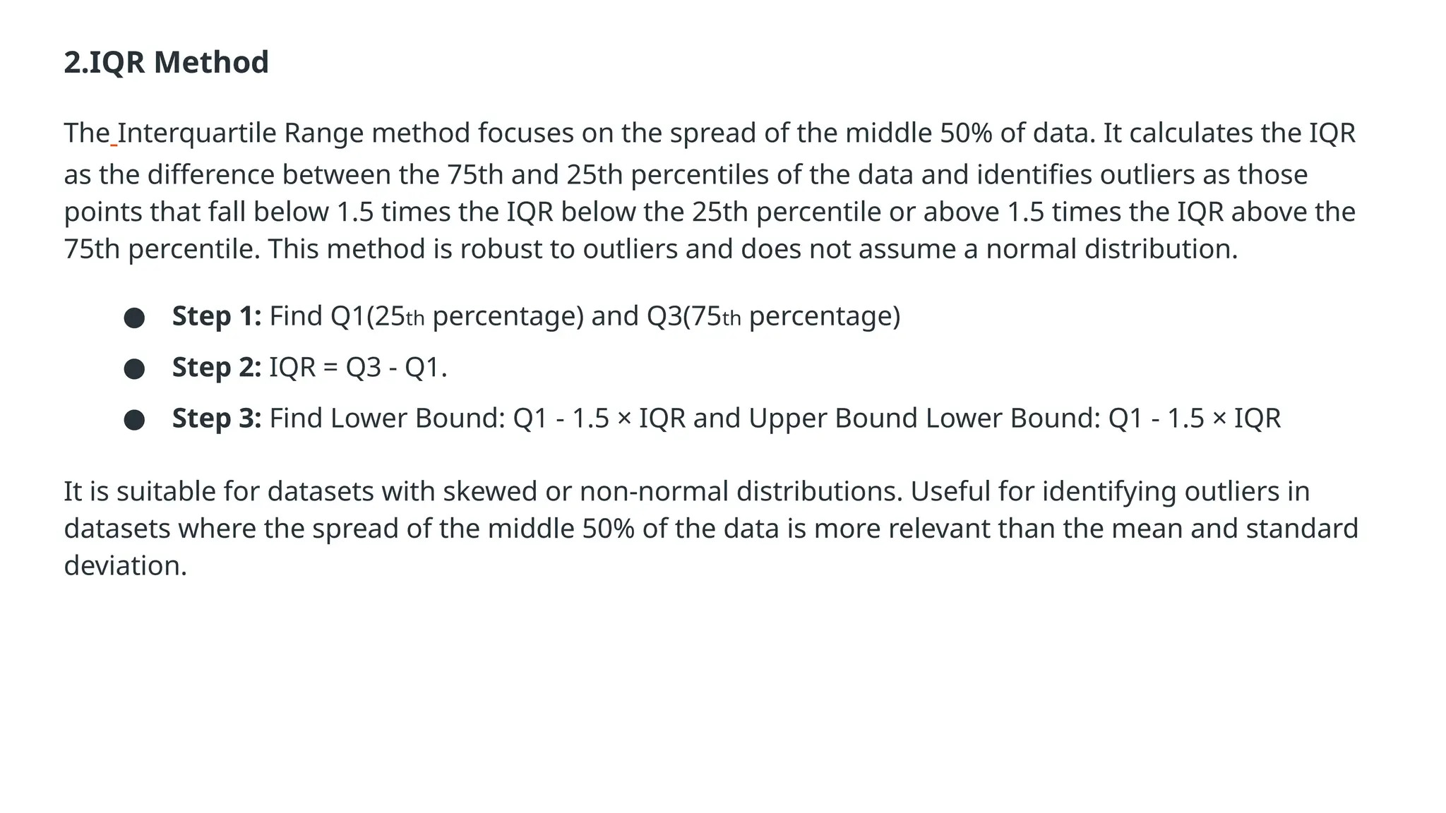
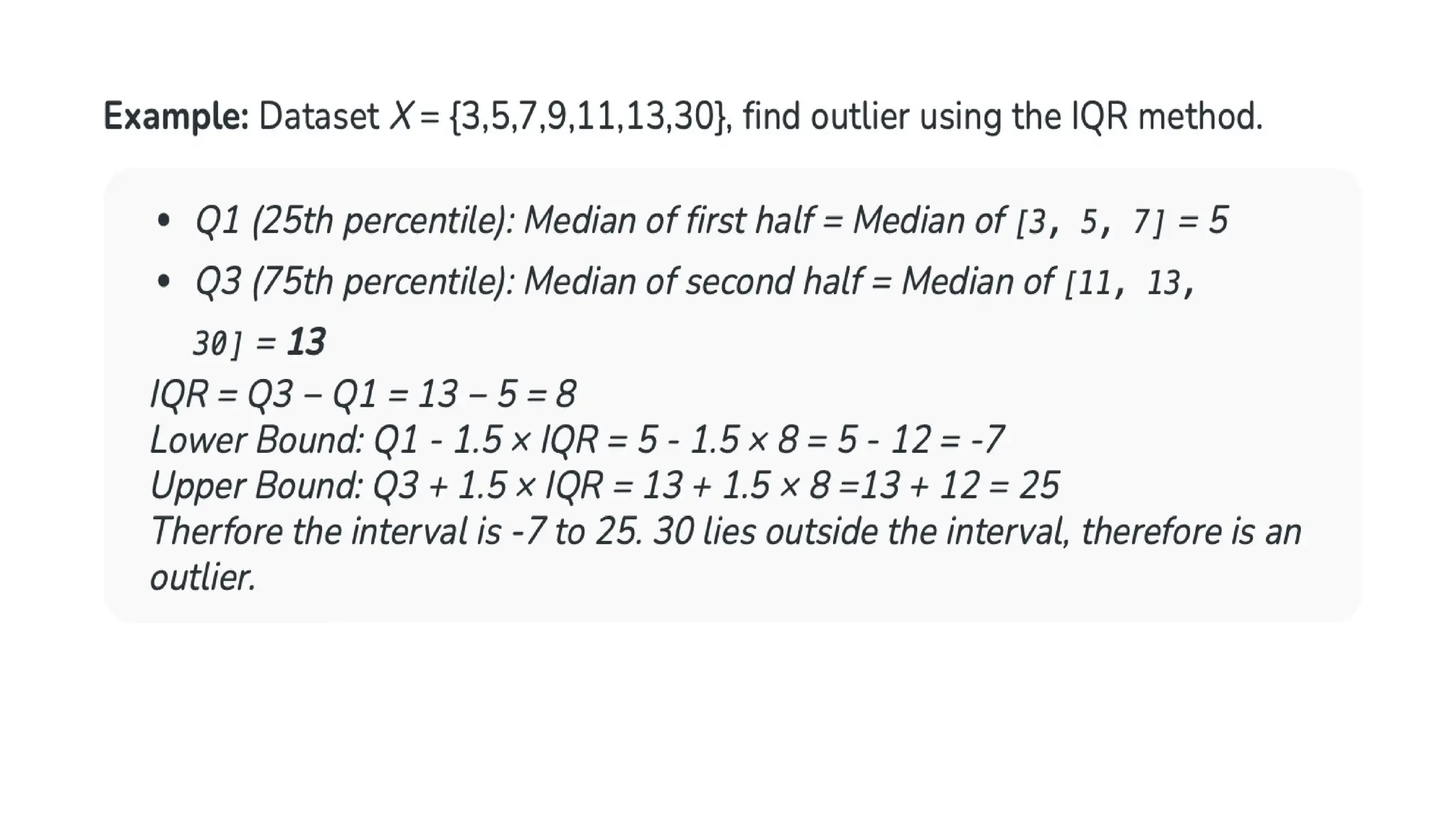
2.IQR Method The Interquartile Range method focuses on the spread of the middle 50% of data. It calculates the IQR as the difference between the 75th and 25th percentiles of the data and identifies outliers as those points that fall below 1.5 times the IQR below the 25th percentile or above 1.5 times the IQR above the 75th percentile. This method is robust to outliers and does not assume a normal distribution. ● Step 1: Find Q1(25th percentage) and Q3(75th percentage) ● Step 2: IQR = Q3 - Q1. ● Step 3: Find Lower Bound: Q1 - 1.5 × IQR and Upper Bound Lower Bound: Q1 - 1.5 × IQR It is suitable for datasets with skewed or non-normal distributions. Useful for identifying outliers in datasets where the spread of the middle 50% of the data is more relevant than the mean and standard deviation.

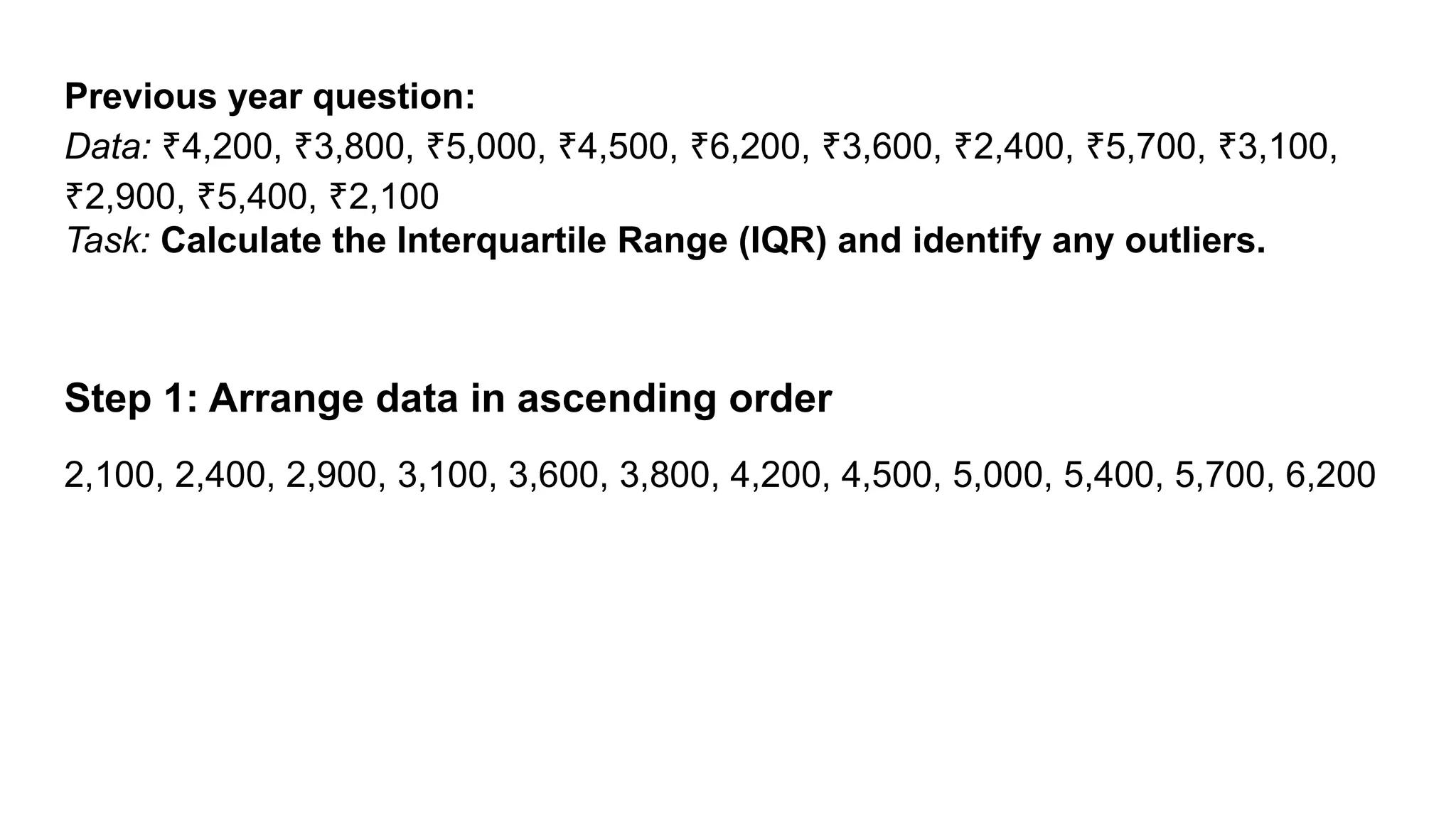
Previous year question: Data: 4,200, 3,800, 5,000, 4,500, 6,200, 3,600, 2,400, 5,700, 3,100, ₹ ₹ ₹ ₹ ₹ ₹ ₹ ₹ ₹ 2,900, 5,400, 2,100 ₹ ₹ ₹ Task: Calculate the Interquartile Range (IQR) and identify any outliers. Step 1: Arrange data in ascending order 2,100, 2,400, 2,900, 3,100, 3,600, 3,800, 4,200, 4,500, 5,000, 5,400, 5,700, 6,200

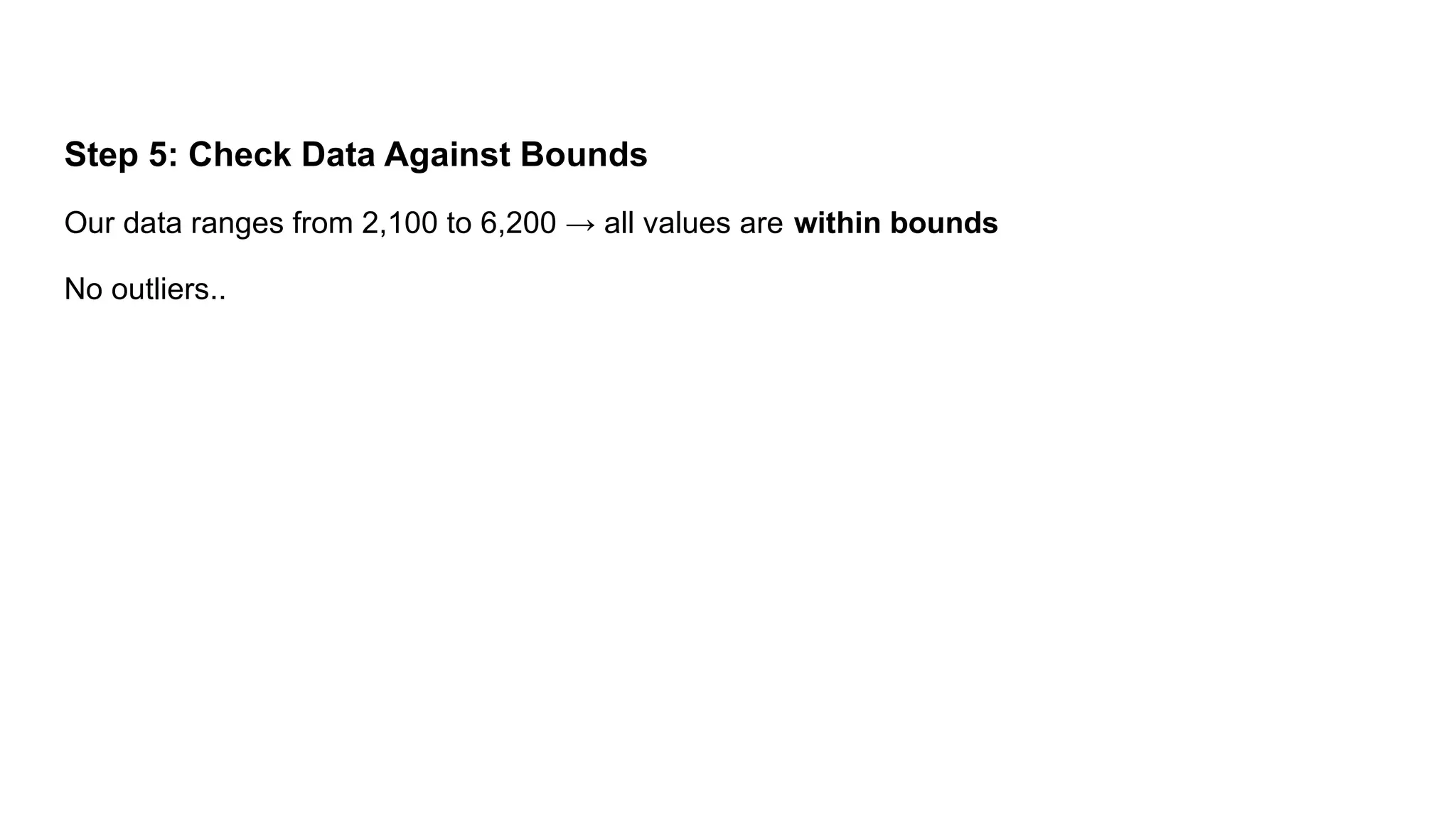
Step 3: Calculate IQR IQR=Q3−Q1=5300−2950=2350 Step 4: Find Outlier Boundaries ● Lower Bound = Q1 – 1.5 × IQR =2950–(1.5×2350)=2950–3525=−575 (Anything below –575 is an outlier → impossible here) ● Upper Bound = Q3 + 1.5 × IQR =5300+(1.5×2350)=5300+3525=8825 (Anything above 8,825 is an outlier)

Step 5: Check Data Against Bounds Our data ranges from 2,100 to 6,200 → all values are within bounds No outliers..

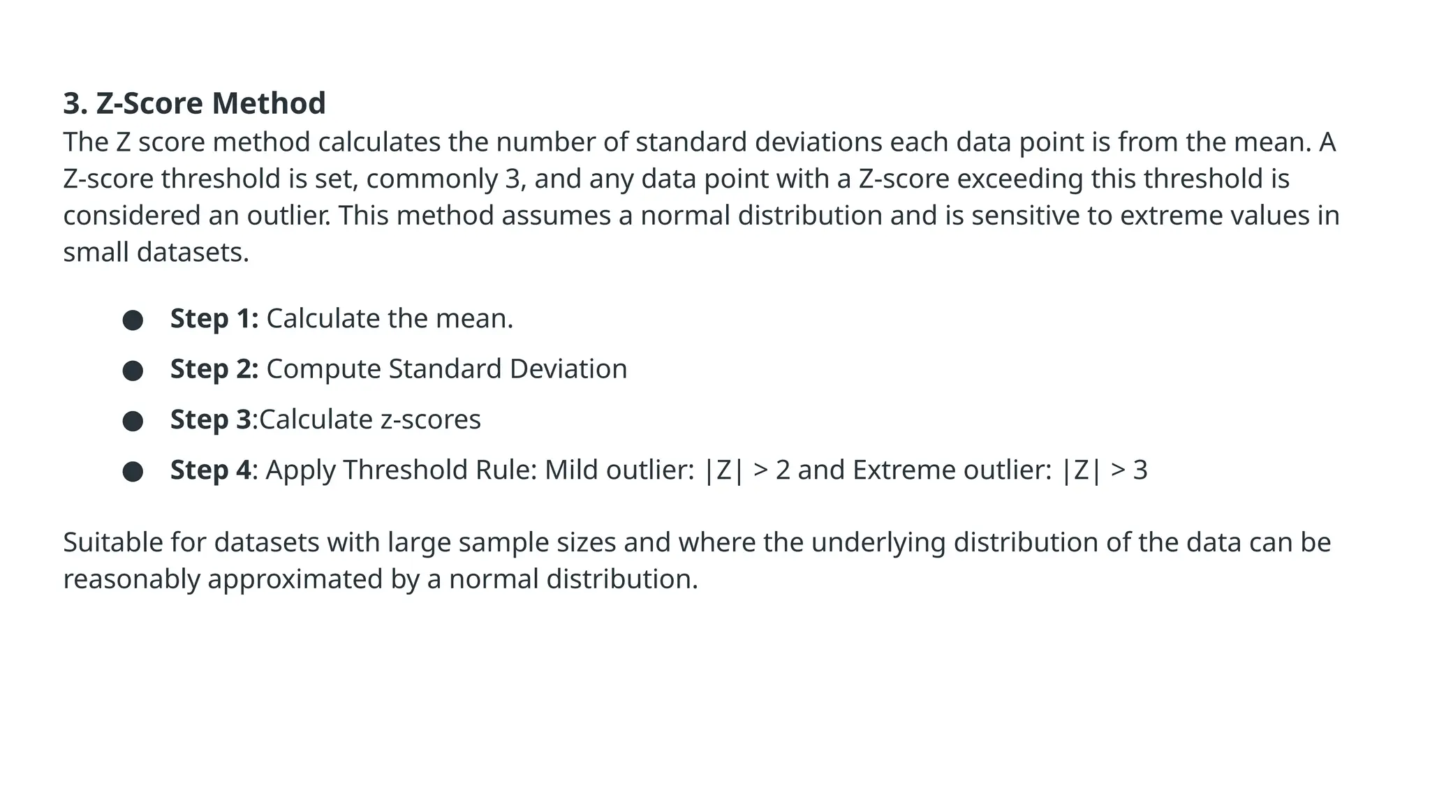
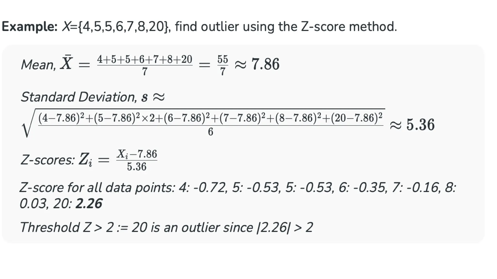
3. Z-Score Method The Z score method calculates the number of standard deviations each data point is from the mean. A Z-score threshold is set, commonly 3, and any data point with a Z-score exceeding this threshold is considered an outlier. This method assumes a normal distribution and is sensitive to extreme values in small datasets. ● Step 1: Calculate the mean. ● Step 2: Compute Standard Deviation ● Step 3:Calculate z-scores ● Step 4: Apply Threshold Rule: Mild outlier: |Z| > 2 and Extreme outlier: |Z| > 3 Suitable for datasets with large sample sizes and where the underlying distribution of the data can be reasonably approximated by a normal distribution.

Challenges with Outlier Detection Detecting outliers effectively poses several challenges: ● Determining the Threshold: Deciding the correct threshold that accurately separates outliers from normal data is critical and difficult. ● Distinguishing Noise from Outliers: In datasets with high variability or noise, it can be particularly challenging to differentiate between noise and actual outliers. ● Balancing Sensitivity: An overly aggressive approach to detecting outliers might eliminate valid data, reducing the richness of the dataset.

Applications of Outlier Detection Outlier detection plays a crucial role across various domains, enabling the identification of anomalies that can indicate errors, fraud, or novel insights. Here are some key applications of outlier detection with specific examples: 1. Financial Fraud Detection ● Fraud Detection: Outlier detection is extensively used in the financial sector to identify fraudulent activities. For instance, credit card companies use outlier detection algorithms to flag unusual spending patterns that may indicate stolen card usage. ● Example: A credit card transaction for a large amount in a foreign country when the cardholder usually makes small, local purchases could be flagged as an outlier, triggering a fraud alert.

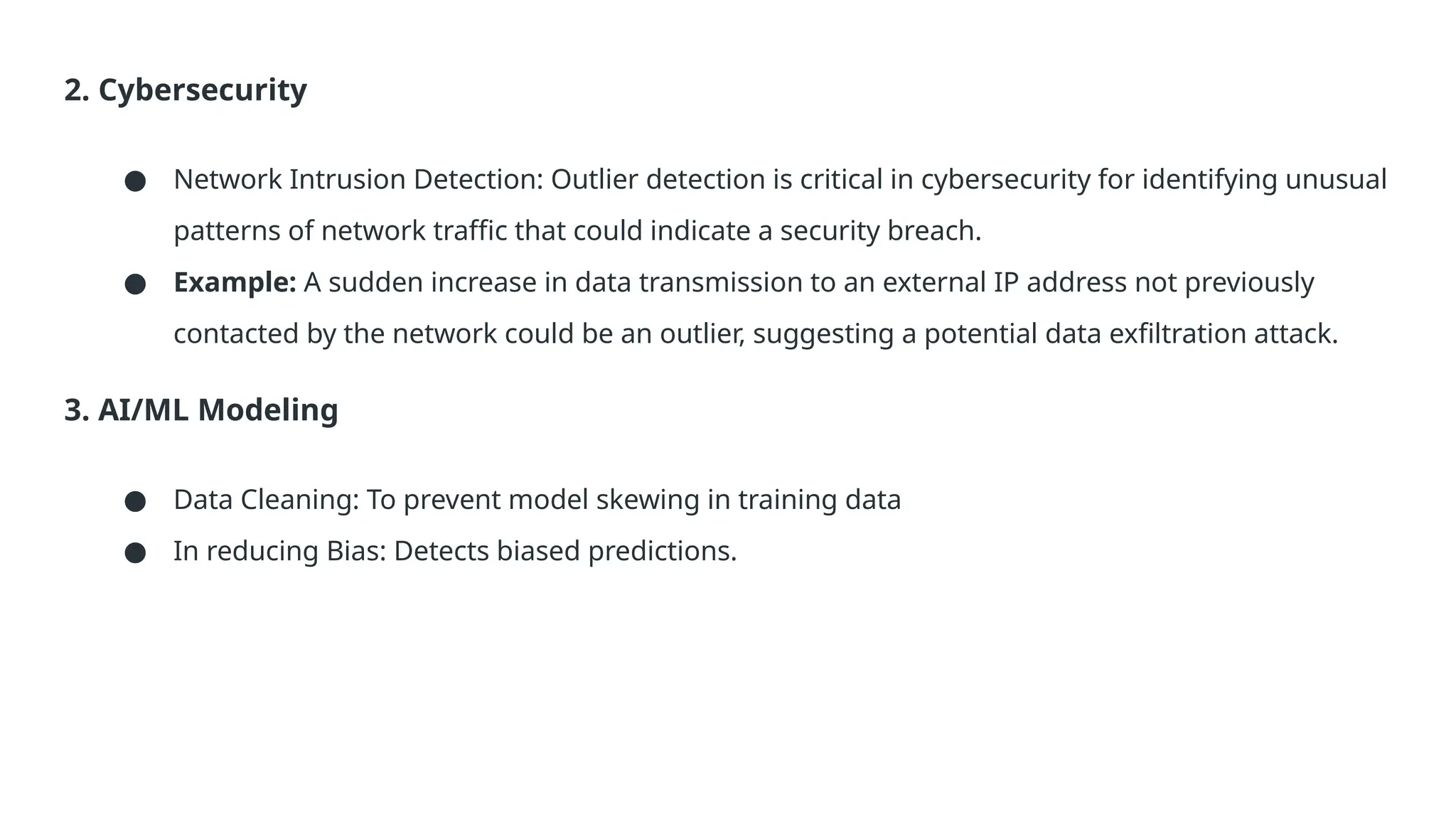
2. Cybersecurity ● Network Intrusion Detection: Outlier detection is critical in cybersecurity for identifying unusual patterns of network traffic that could indicate a security breach. ● Example: A sudden increase in data transmission to an external IP address not previously contacted by the network could be an outlier, suggesting a potential data exfiltration attack. 3. AI/ML Modeling ● Data Cleaning: To prevent model skewing in training data ● In reducing Bias: Detects biased predictions.

4. Anomaly Detection in Big Data & Cloud Systems ● Cloud Security: To detect unauthorized access in large-scale cloud environments. ● Ensures integrity by flagging corrupted entries.

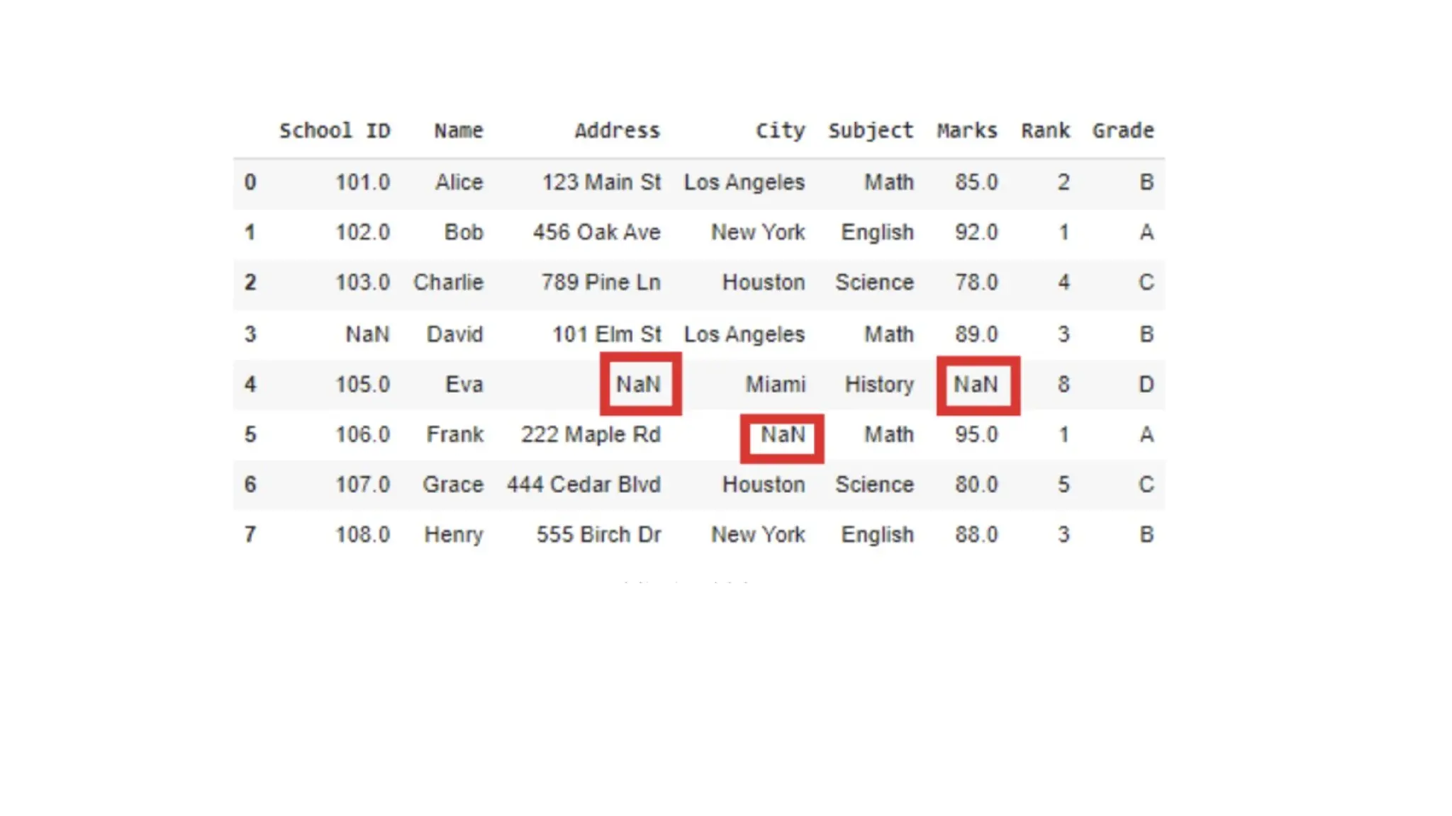
Handling Missing Values Missing values are a common challenge in machine learning and data analysis. They occur when certain data points are missing for specific variables in a dataset. These gaps in information can take the form of blank cells, null values or special symbols like "NA", "NaN" or "unknown." If not addressed properly, missing values can harm the accuracy and reliability of our models. They can reduce the sample size, introduce bias and make it difficult to apply certain analysis techniques that require complete data. Efficiently handling missing values is important to ensure our machine learning models produce accurate and unbiased results.

Importance of Handling Missing Values Handling missing values is important for ensuring the accuracy and reliability of data analysis and machine learning models. Key reasons include: ● Improved Model Accuracy: Addressing missing values helps avoid incorrect predictions and boosts model performance. ● Increased Statistical Power: Imputation or removal of missing data allows the use of more analysis techniques, maintaining the sample size. ● Bias Prevention: Proper handling ensures that missing data doesn’t introduce systematic bias, leading to more reliable results. ● Better Decision-Making: A clean dataset leads to more informed, trustworthy decisions based on accurate insights.

Challenges Posed by Missing Values Missing values can introduce several challenges in data analysis including: ● Reduce sample size: If rows or data points with missing values are removed, it reduces the overall sample size which may decrease the reliability and accuracy of the analysis. ● Bias in Results: When missing data is not handled carefully, it can introduce bias. This is especially problematic when the missingness is not random, leading to misleading conclusions. ● Difficulty in Analysis: Many statistical techniques and machine learning algorithms require complete data for all variables. Missing values can cause certain analyses or models inapplicable, limiting the methods we can use.

Reasons Behind Missing Values in the Dataset Data can be missing from a dataset for several reasons and understanding the cause is important for selecting the most effective way to handle it. Common reasons for missing data include: ● Technical issues: Failed data collection or errors during data transmission. ● Human errors: Mistakes like incorrect data entry or oversights during data processing. ● Privacy concerns: Missing sensitive or personal information due to confidentiality policies. ● Data processing issues: Errors that occur during data preparation. By identifying the reason behind the missing data, we can better assess its impact whether it's causing bias or affecting the analysis and select the proper handling method such as imputation or removal.

Types of Missing Values Missing values in a dataset can be categorized into three main types each with different implications for how they should be handled: 1. Missing Completely at Random (MCAR): In this case, the missing data is completely random and unrelated to any other variable in the dataset. The absence of data points occurs without any systematic pattern such as a random technical failure or data omission. 2. Missing at Random (MAR): The missingness is related to other observed variables but not to the value of the missing data itself. For example, if younger individuals are more likely to skip a particular survey question, the missingness can be explained by age but not by the content of the missing data. 3. Missing Not at Random (MNAR): Here, the probability of missing data is related to the value of the missing data itself. For example, people with higher incomes may be less likely to report their income, leading to a direct connection between the missingness and the value of the missing data.

Variables , outlier and its detection and Missing values

Variables , outlier and its detection and Missing values

More Related Content

Similar to Variables , outlier and its detection and Missing values

Recently uploaded

Variables , outlier and its detection and Missing values