Using R for Building a Simple and Effective Dashboard

How to use open source tools and data science to get insights on business and customers

 The goal of this talk is  Give you a flavour of what can you do with open source data analysis tools like R or Python  Give you some useful «code snippets» to make practice  Provide a way of reasoning while commenting code and slides

 The setting  You are a rampant Data Scientist  Someone want to start a new business in NY and create a taxi company (or the new Uber!) and ask you an advice  You want to prepare a beautiful and simple dashboard with the most relevant insights and KPI

 First think first… Get some Data  http://www.nyc.gov/html/tlc/html/home/home.shtml

Customer behaviour Economics Insights & Graphics Other Insights  Sketch an idea of your Dashboard/Report

 Start Exploring Data  Trip Details Data ▪ medallion, hack_license, vendor_id, rate_code, store_and_fwd_flag, Pickup_datetime, Drop- off_datetime, passenger_count, trip_time_in_secs, trip_distance, Pickup_longitude, Pickup_latitude, Drop- off_longitude, Drop-off_latitude  Trip Fare Data: ▪ medallion, hack_license, vendor_id, Pickup_datetime, payment_type, fare_amount, surcharge, mta_tax, tip_amount, tolls_amount, total_amount

In the following I’ll make extensive use of R (https://www.r-project.org), Rstudio (https://www.rstudio.com) and the following R libraries library(psych) library(dplyr) library(ggmap) library(lattice)

 Download data in <your folder> from here:  Unzip  Import in a R DataFrame: setwd(“<your folder>") Import them in a Dataframe: #read trip_data.csv data_trip<-read.csv("trip_data.csv",sep=',', header=1,nrows=500000) #read trip_fare.csv data_fares<-read.csv("trip_fare.csv",sep=',‘, header=1,nrows=500000)

 Let’s do some Cleansing, for example #exclude trip with time less than 60 seconds data_trip<-data_trip[( data_trip$trip_time_in_secs)>60,] #exclude trip with distance less than 0.1 miles data_trip<-data_trip[( data_trip$trip_distance)>0.1,] data_trip<-data_trip [!(data_trip$pickup_latitude==0 | data_trip$pickup_longitude==0),]

#work on a selection of the NYC area data_trip<-data_trip[( data_trip$pickup_latitude>(40.62)& data_trip$pickup_latitude<40.9 & data_trip$pickup_longitude>(-74.1)& data_trip$pickup_longitude<(-73.75)& data_trip$dropoff_latitude>(40.62)& data_trip$dropoff_latitude<40.9& data_trip$dropoff_longitude>(-74.1)& data_trip$dropoff_longitude<(73.75)) ,]

 Build new variables, #create a column for pickup_hour data_trip$pickup_hour<-as.POSIXlt( data_trip$pickup_datetime)$hour #create a column for dropoff_hour data_trip$dropoff_hour<-as.POSIXlt( data_trip$dropoff_datetime)$hour #create a column for counting data_trip$ones<-1

 Remove some variables, data_fares$medallion<-NULL data_fares$vendor_id<-NULL data_trip$dropoff_datetime<-NULL data_trip$medallion<-NULL data_trip$vendor_id<-NULL data_trip$store_and_fwd_flag<-NULL data_trip$rate_code<-NULL

 Plot some Histograms #Distribution of number of passengers per trip hist(data_trip$passenger_count,6, main="Distribution of Number of Passengers per Trip",xlab="Number of Passengers p/Trip") rect(par("usr")[1], par("usr")[3], par("usr")[2], par("usr")[4], col = "grey") hist(data_trip$passenger_count,6, add = TRUE,col=" lightgoldenrod2 ")

#Distribution of payment_type barplot(sort(table(data_fares$payment_type), decreasing = TRUE), xaxt = 'n') rect(par("usr")[1], par("usr")[3], par("usr")[2], par("usr")[4], col = "grey") barplot(sort(table(data_fares$payment_type), decreasing = TRUE), ylab="Frequency“, col="lightgoldenrod2", add =TRUE, main="Distribution of Payement Type“)

#Distribution of number of trip time length hist(data_trip$trip_time_in_secs/60,10, xlim=c(0,100),main="Distribution of Trip Time",xlab="Trip Time in minutes") rect(par("usr")[1], par("usr")[3], par("usr")[2], par("usr")[4], col = "grey") hist(data_trip$trip_time_in_secs/60,10, add = TRUE,col="lightgoldenrod2")

#Distribution of number of trip distance hist(data_trip$trip_distance,100,xlim=c(0,40), main="Distribution of Trip Distance", xlab="Trip Distance") rect(par("usr")[1], par("usr")[3], par("usr")[2], par("usr")[4], col = "grey") hist(data_trip$trip_distance,100, add =TRUE, col="lightgoldenrod2")

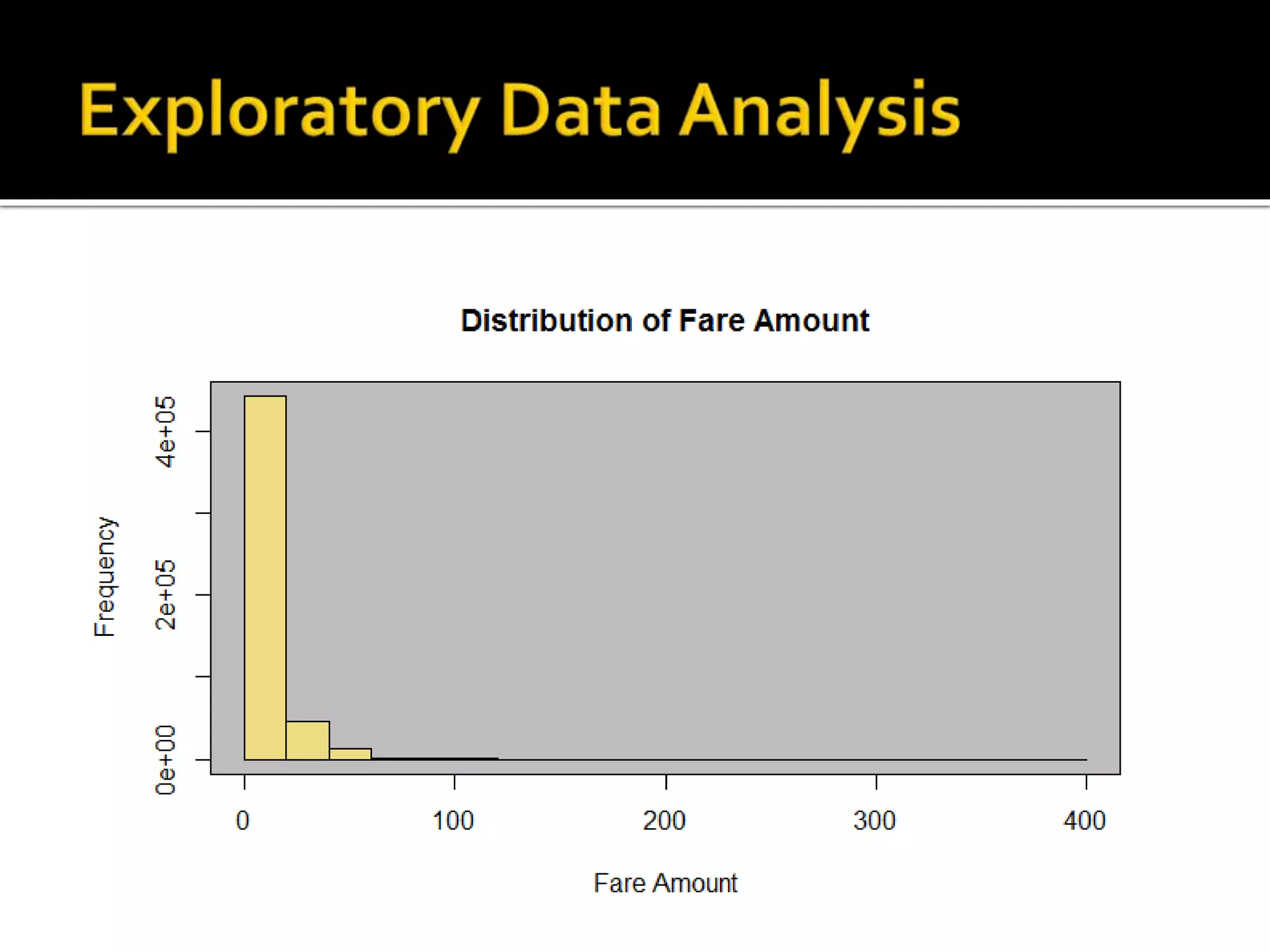
#Distribution of fare amount (full domain) hist(data_fares$fare_amount, main="Distribution of Fare Amount", xlab="Fare Amount") rect(par("usr")[1], par("usr")[3], par("usr")[2], par("usr")[4], col = "grey") hist(data_fares$fare_amount,add = TRUE,col="lightgoldenrod2")

#Distribution of fare amount (restricted domain) hist(data_fares$fare_amount,xlim=c(0,80),200, main="Distribution of Fare Amount", xlab="Fare Amount") rect(par("usr")[1], par("usr")[3], par("usr")[2], par("usr")[4], col = "grey“) hist(data_fares$fare_amount,200, xlim=c(0,80),add = TRUE,col="lightgoldenrod2")

#Distribution of tip amount hist(data_fares$tip_amount,500,xlim=c(0,20), main="Distribution of Tip Amount", xlab="Tip Amount") rect(par("usr")[1], par("usr")[3], par("usr")[2], par("usr")[4], col = "grey") hist(data_fares$tip_amount,500,xlim=c(0,20),add = TRUE,col="lightgoldenrod2")

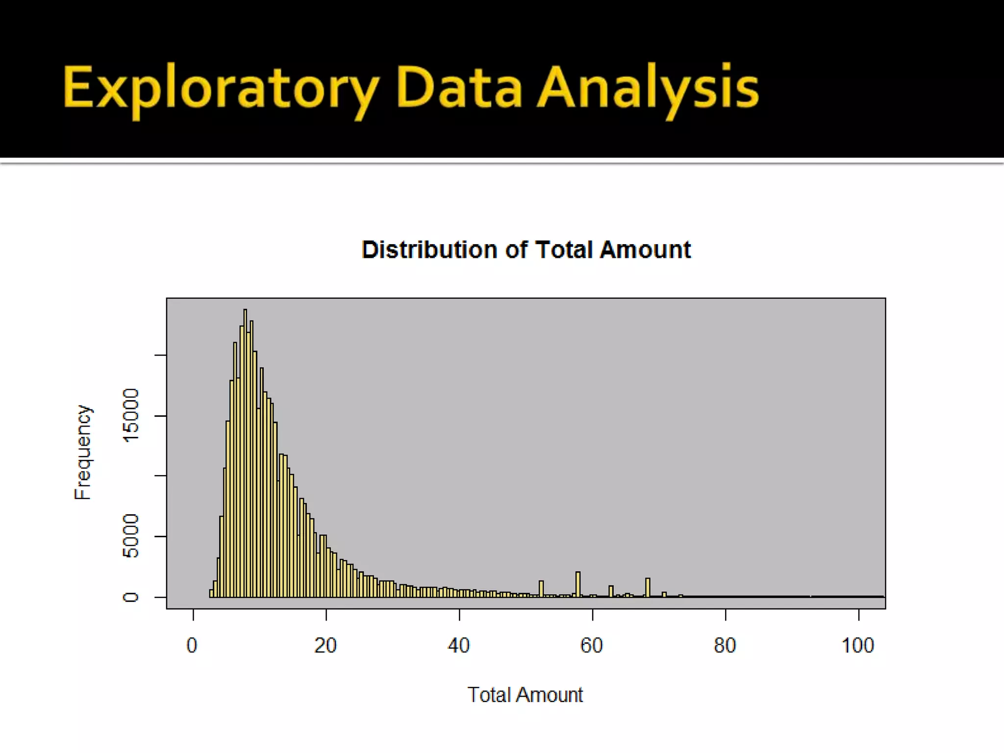
#Distribution of Total Amount hist(data_fares$total_amount,1000,xlim=c(0,100), main="Distribution of Total Amount", xlab="Total Amount") rect(par("usr")[1], par("usr")[3], par("usr")[2], par("usr")[4], col = "grey") hist(data_fares$total_amount,add = TRUE, col="lightgoldenrod2",1000,xlim=c(0,100))

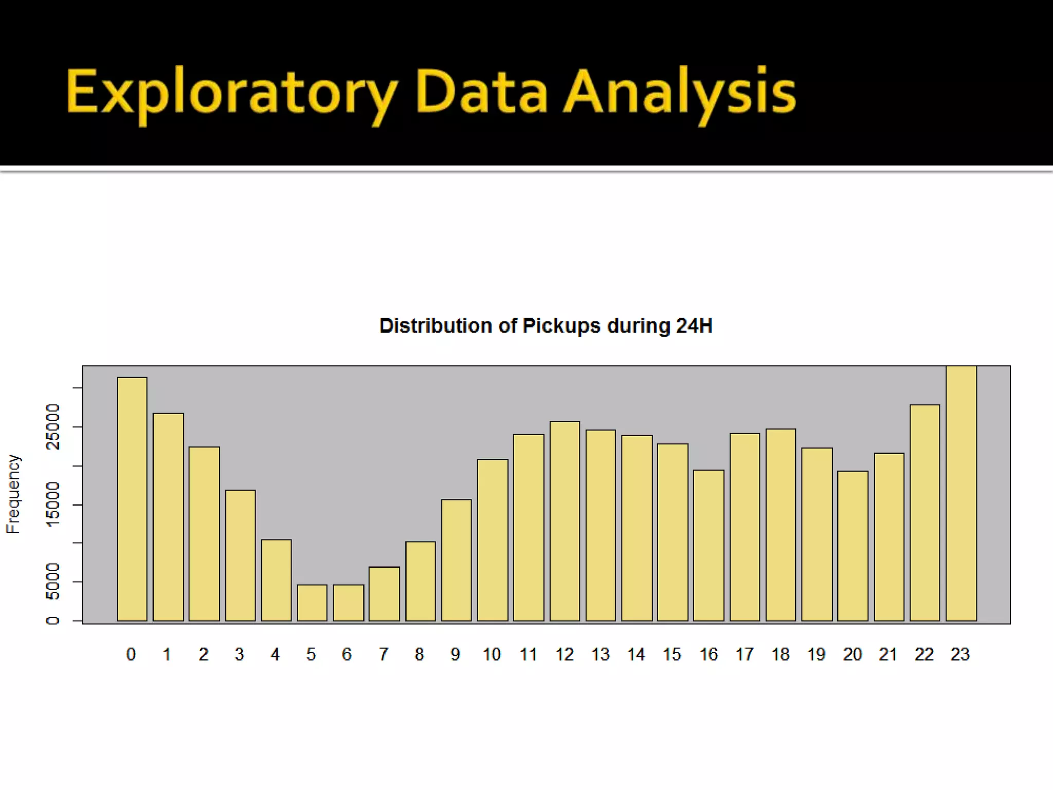
#Distribution of pickups during the day barplot(table(data_trip$pickup_hour)) rect(par("usr")[1], par("usr")[3], par("usr")[2], par("usr")[4], col = "grey") barplot(table(data_trip$pickup_hour), add = TRUE, col="lightgoldenrod2", main="Distribution of Pickups in 24H", ylab="Frequency")

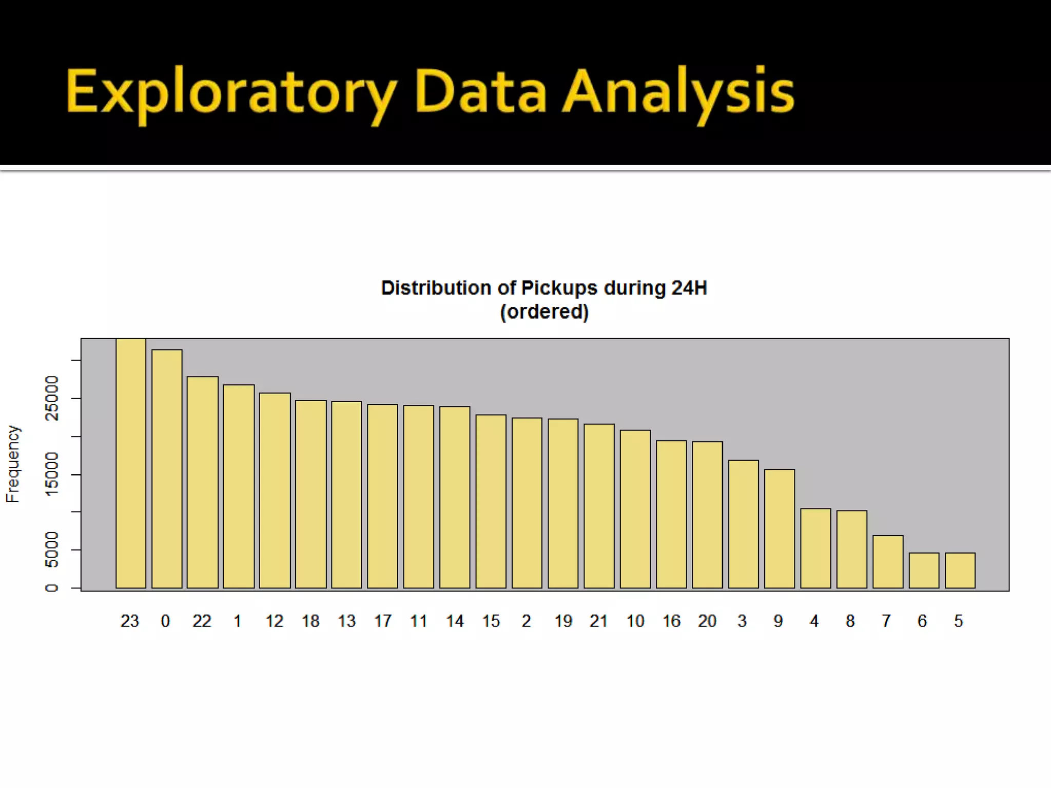
#Distribution of pickups during the day (ordered) barplot(sort(table(data_trip$pickup_hour), decreasing = TRUE)) rect(par("usr")[1], par("usr")[3], par("usr")[2], par("usr")[4], col = "grey") barplot(sort(table(data_trip$pickup_hour), decreasing = TRUE)),add = TRUE, col="lightgoldenrod2", main="Distribution of Pickups in 24H", ylab="Frequency")

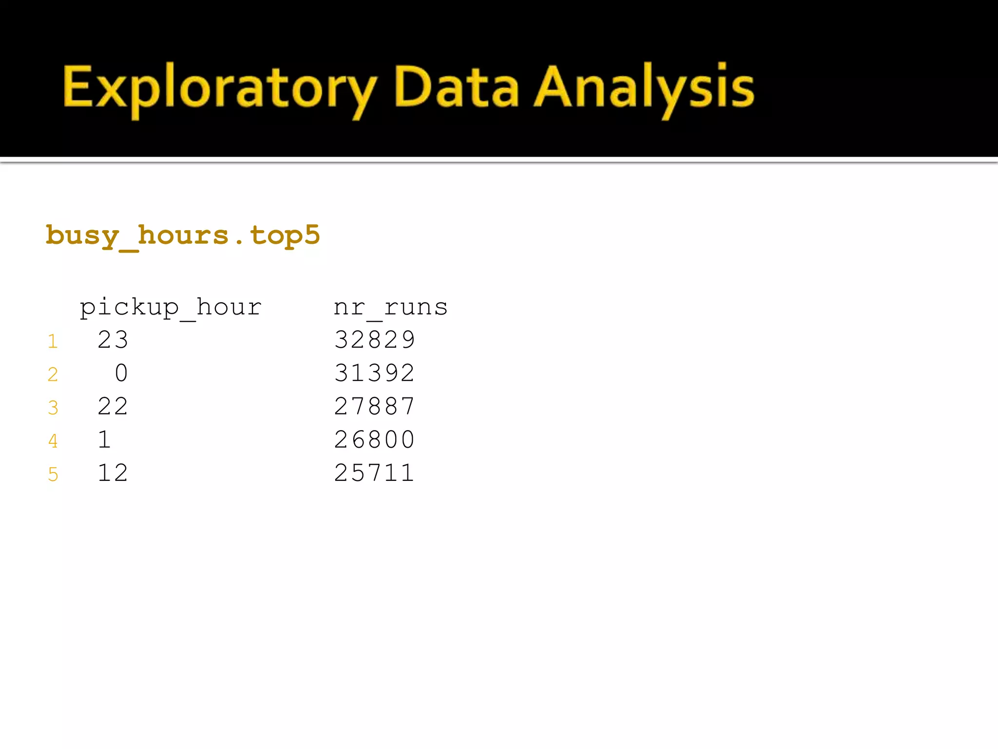
#Top 5 busiest hours of the day busy_hours<-aggregate(data_trip$ones ~ data_trip$pickup_hour, data_trip, sum) #select top 5 pickup_hours busy_hours.top5<- busy_hours %>% arrange(desc(busy_hours[,2])) %>% top_n(5) names(busy_hours.top5)[names(busy_hours.top5)== "data_trip$pickup_hour"]<-"pickup_hour" names(busy_hours.top5)[names(busy_hours.top5)== "data_trip$ones"] <- "nr_runs"

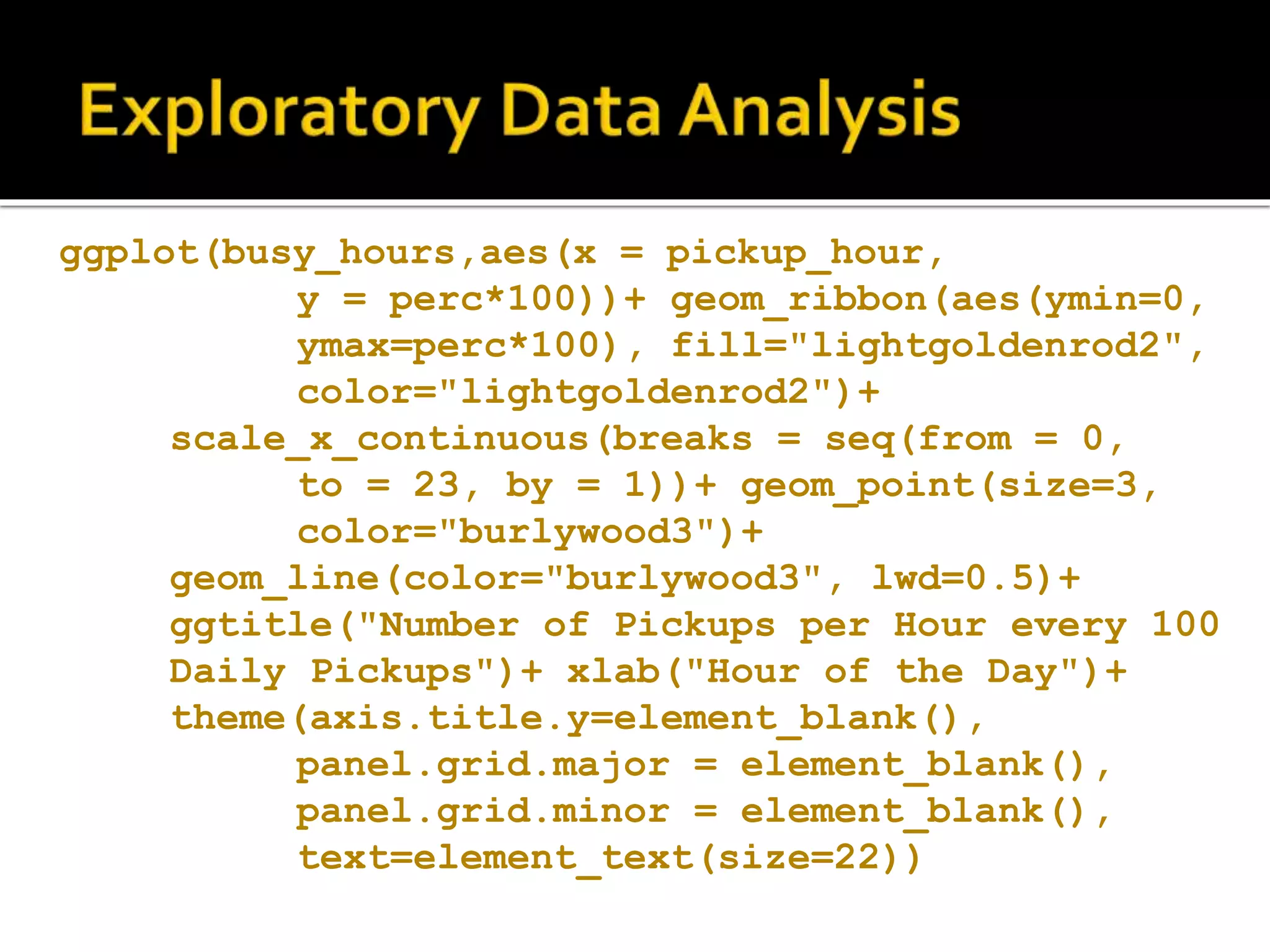
busy_hours.top5 pickup_hour nr_runs 1 23 32829 2 0 31392 3 22 27887 4 1 26800 5 12 25711

#Distribution of pickups during the day in % names(busy_hours)[names(busy_hours)== "data_trip$pickup_hour"]<-"pickup_hour“ names(busy_hours)[names(busy_hours)== "data_trip$ones"] <- "counter“ hoursum<-sum(busy_hours$counter) busy_hours$perc<-busy_hours$counter/hoursum

ggplot(busy_hours,aes(x = pickup_hour, y = perc*100))+ geom_ribbon(aes(ymin=0, ymax=perc*100), fill="lightgoldenrod2", color="lightgoldenrod2")+ scale_x_continuous(breaks = seq(from = 0, to = 23, by = 1))+ geom_point(size=3, color="burlywood3")+ geom_line(color="burlywood3", lwd=0.5)+ ggtitle("Number of Pickups per Hour every 100 Daily Pickups")+ xlab("Hour of the Day")+ theme(axis.title.y=element_blank(), panel.grid.major = element_blank(), panel.grid.minor = element_blank(), text=element_text(size=22))

#Top 10 busiest locations of the city #Build variables to define «locations» data_trip$latpickup<- round(data_trip$pickup_latitude/0.005)*0.005 data_trip$slatpickup<- lapply(data_trip$latpickup,toString) data_trip$lonpickup<- round(data_trip$pickup_longitude/0.005)*0.005 data_trip$slonpickup<- lapply(data_trip$lonpickup,toString) data_trip$trip_start<- paste(data_trip$slatpickup, data_trip$slonpickup,sep="|")

#build a trip identifier concatenating rounded #latitude and longitude in string format data_trip$trip_start<-paste(data_trip$slatpickup, data_trip$slonpickup,sep="|") #get rid of unuseful variables data_trip$latpickup<-NULL data_trip$lonpickup<-NULL data_trip$slatpickup<-NULL data_trip$slonpickup<-NULL

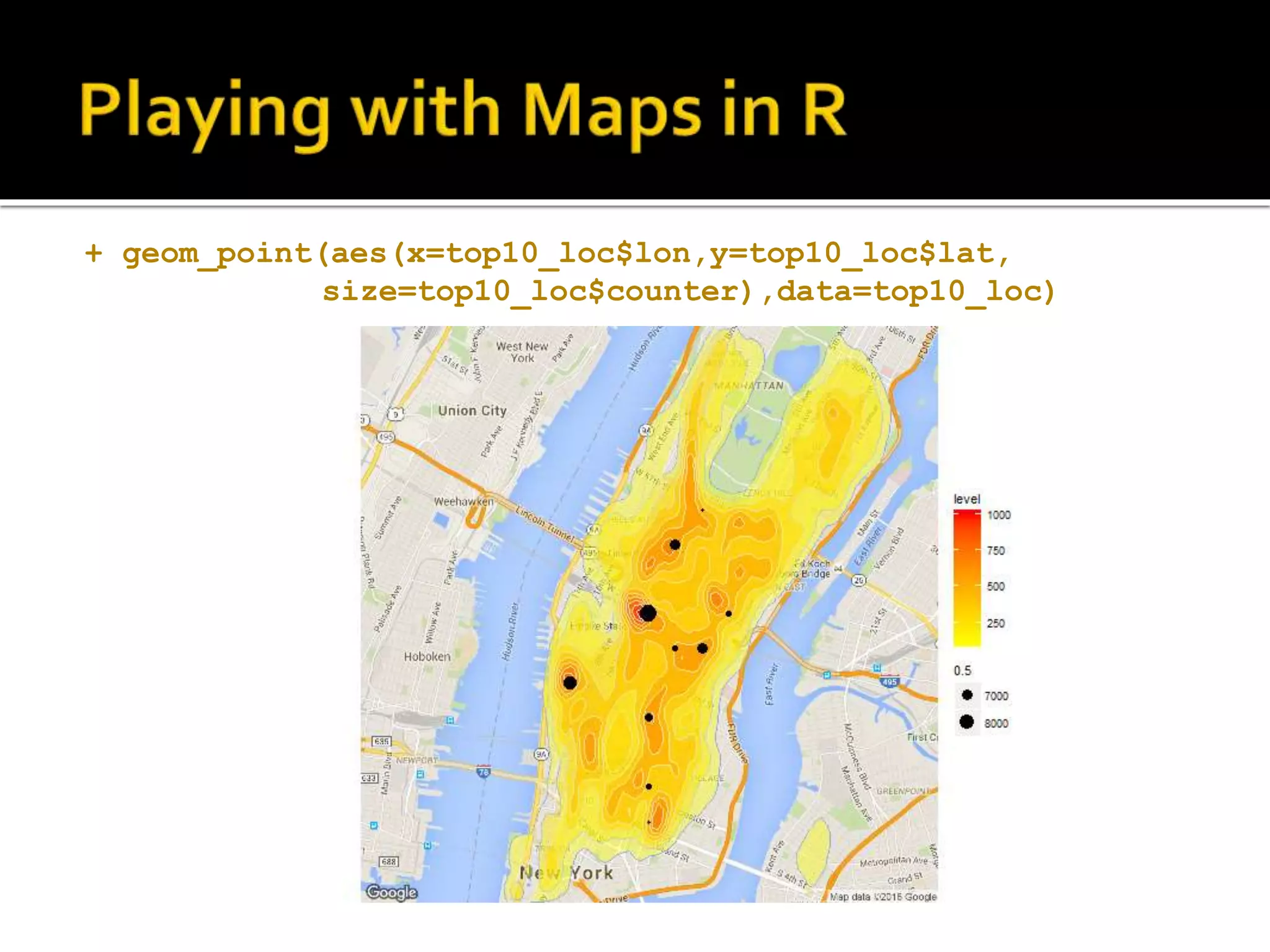
#groupby trip identifier and count busy_locations <- aggregate(data_trip$ones ~ data_trip$trip_start, data_trip, sum) names(busy_locations)[names(busy_locations)== "data_trip$trip_start"] <- "location“ names(busy_locations)[names(busy_locations)== "data_trip$ones"] <- "counter"

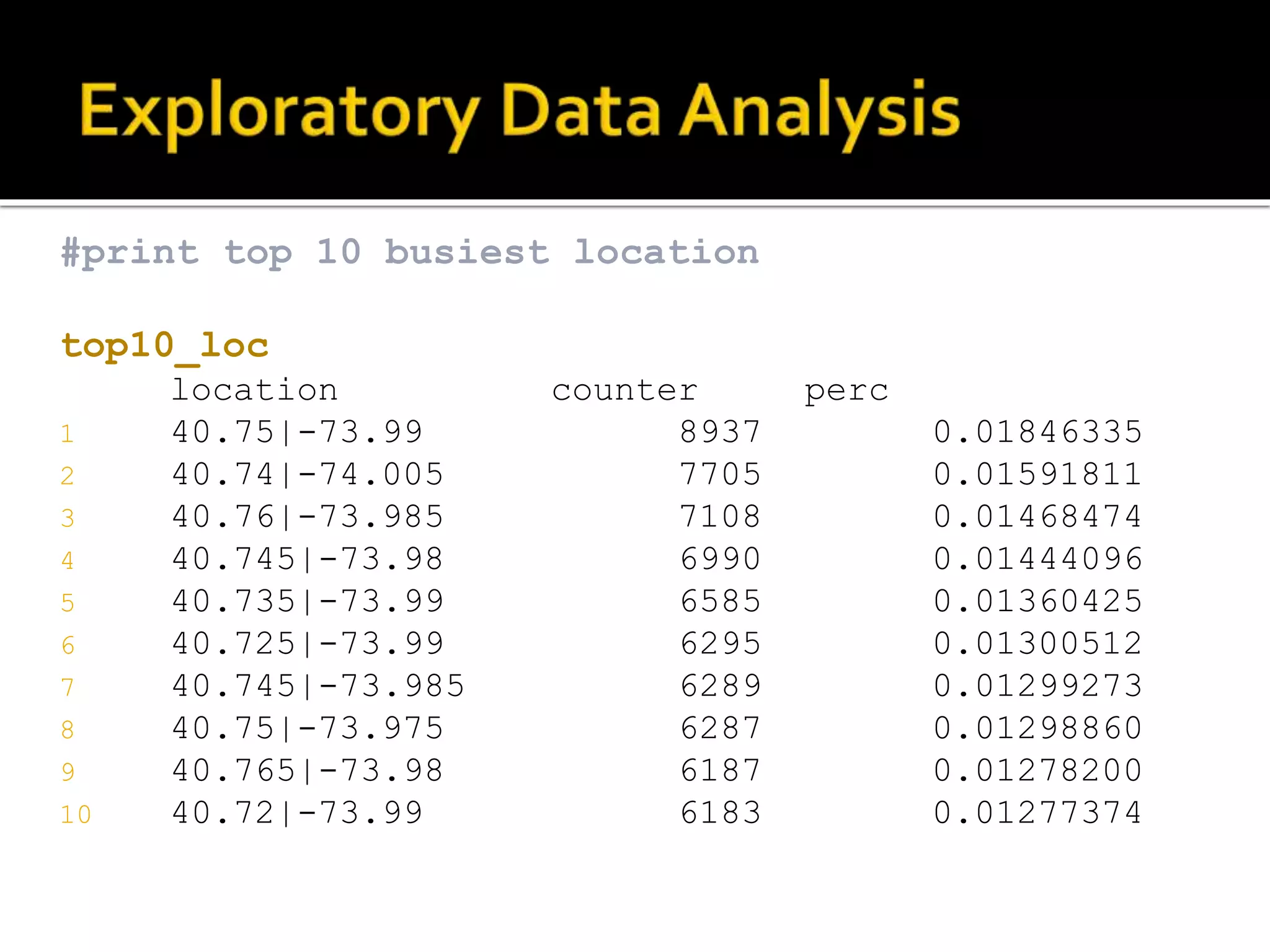
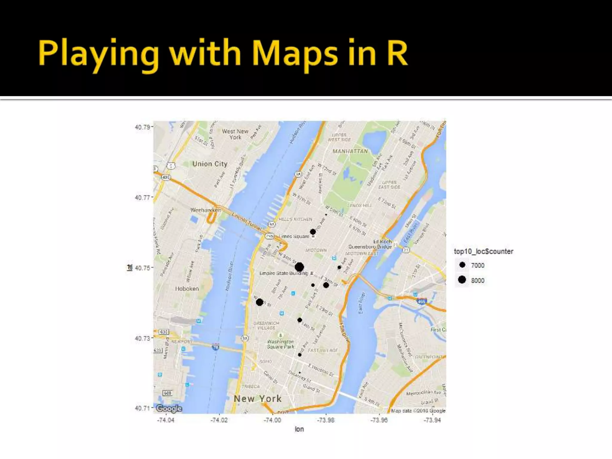
#total number of trip tripsum <- sum(busy_locations$counter) #total number of trip busy_locations$perc <- busy_locations$counter /tripsum top10_loc <- busy_locations %>% arrange( desc(busy_locations[,2])) %>% top_n(10)

#print top 10 busiest location top10_loc location counter perc 1 40.75|-73.99 8937 0.01846335 2 40.74|-74.005 7705 0.01591811 3 40.76|-73.985 7108 0.01468474 4 40.745|-73.98 6990 0.01444096 5 40.735|-73.99 6585 0.01360425 6 40.725|-73.99 6295 0.01300512 7 40.745|-73.985 6289 0.01299273 8 40.75|-73.975 6287 0.01298860 9 40.765|-73.98 6187 0.01278200 10 40.72|-73.99 6183 0.01277374

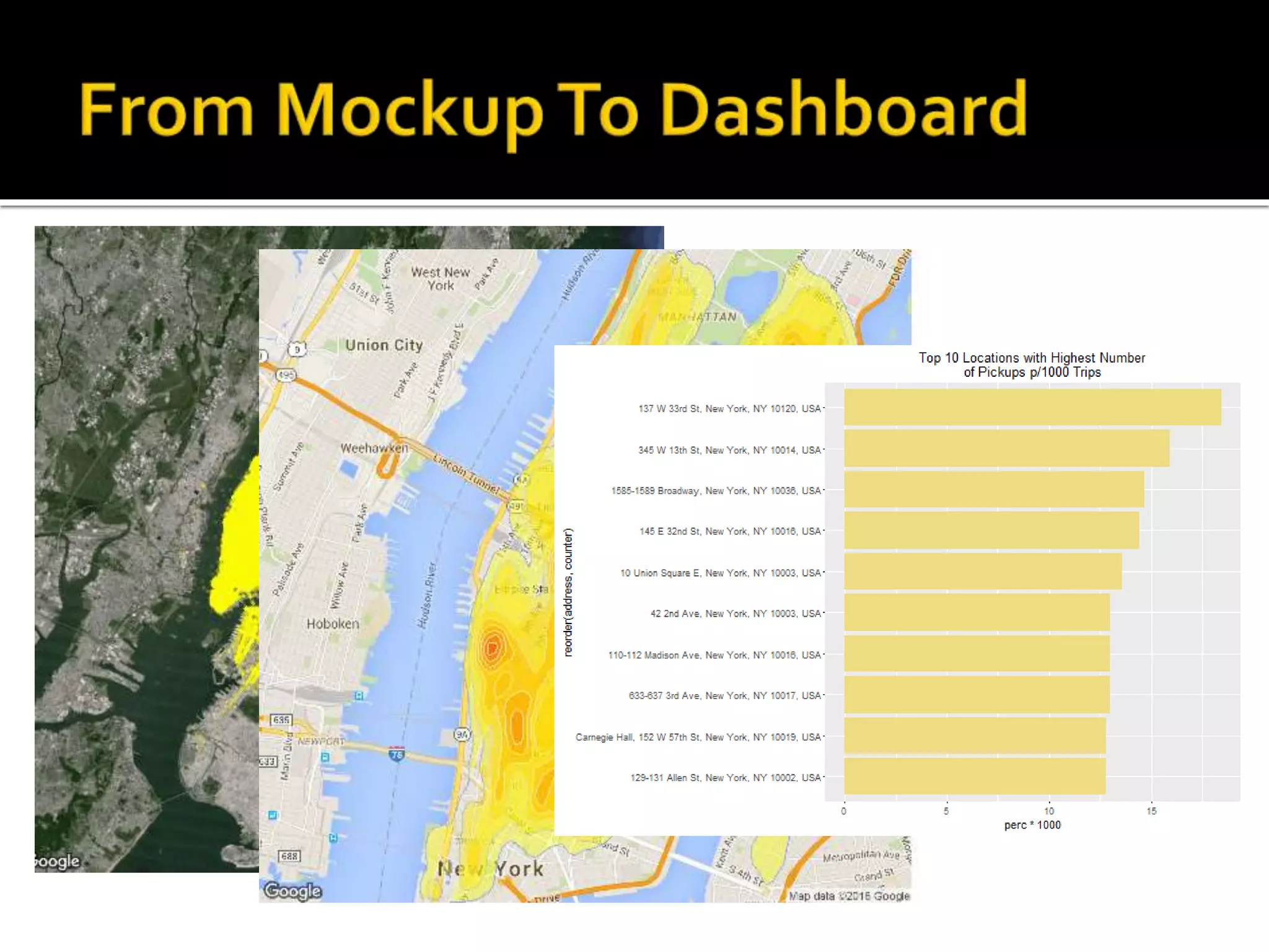
#get address of busy locations C <- unlist(strsplit(top10_loc$location, "[|]")) coordinates = matrix(as.double(c), nrow=10, ncol=2,byrow=TRUE) top10_loc$lat<-coordinates[,1] top10_loc$lon<-coordinates[,2] top10_loc$address<-mapply(FUN = function(lon, lat) revgeocode(c(lon, lat)), top10_loc$lon, top10_loc$lat)

top10_loc$address [1] "137 W 33rd St, New York, NY 10120, USA" [2] "345 W 13th St, New York, NY 10014, USA" [3] "1585-1589 Broadway, New York, NY 10036, USA" [4] "145 E 32nd St, New York, NY 10016, USA" [5] "10 Union Square E, New York, NY 10003, USA" [6] "42 2nd Ave, New York, NY 10003, USA" [7] "110-112 Madison Ave, New York, NY 10016, USA" [8] "633-637 3rd Ave, New York, NY 10017, USA" [9] "Carnegie Hall, 152 W 57th St, New York, NY 10019, USA" [10] "129-131 Allen St, New York, NY 10002, USA"

#represent busiest addresses in a barchart ggplot(top10_loc, aes(x=reorder(address, counter), y=perc*1000)) + geom_bar(stat='identity',fill="lightgoldenrod2") + coord_flip() + ggtitle("Top 10 Locations with Highest Numbernof Pickups p/1000 Trips")

#build map for busy locations ny_map<-get_map(location = c(-73.9308, 40.7336),maptype = "satellite", zoom=11) ny_map2<-get_map(location=c(-73.9874, 40.7539),maptype = "satellite", zoom=13) ny_map3<-get_map(location=c(-73.99,40.75), maptype = "roadmap", zoom=13) #represent busiest location in a map ggmap(ny_map3)+geom_point(aes(x=top10_loc$lon,y=t op10_loc$lat,size=top10_loc$counter),data=top10_l oc)

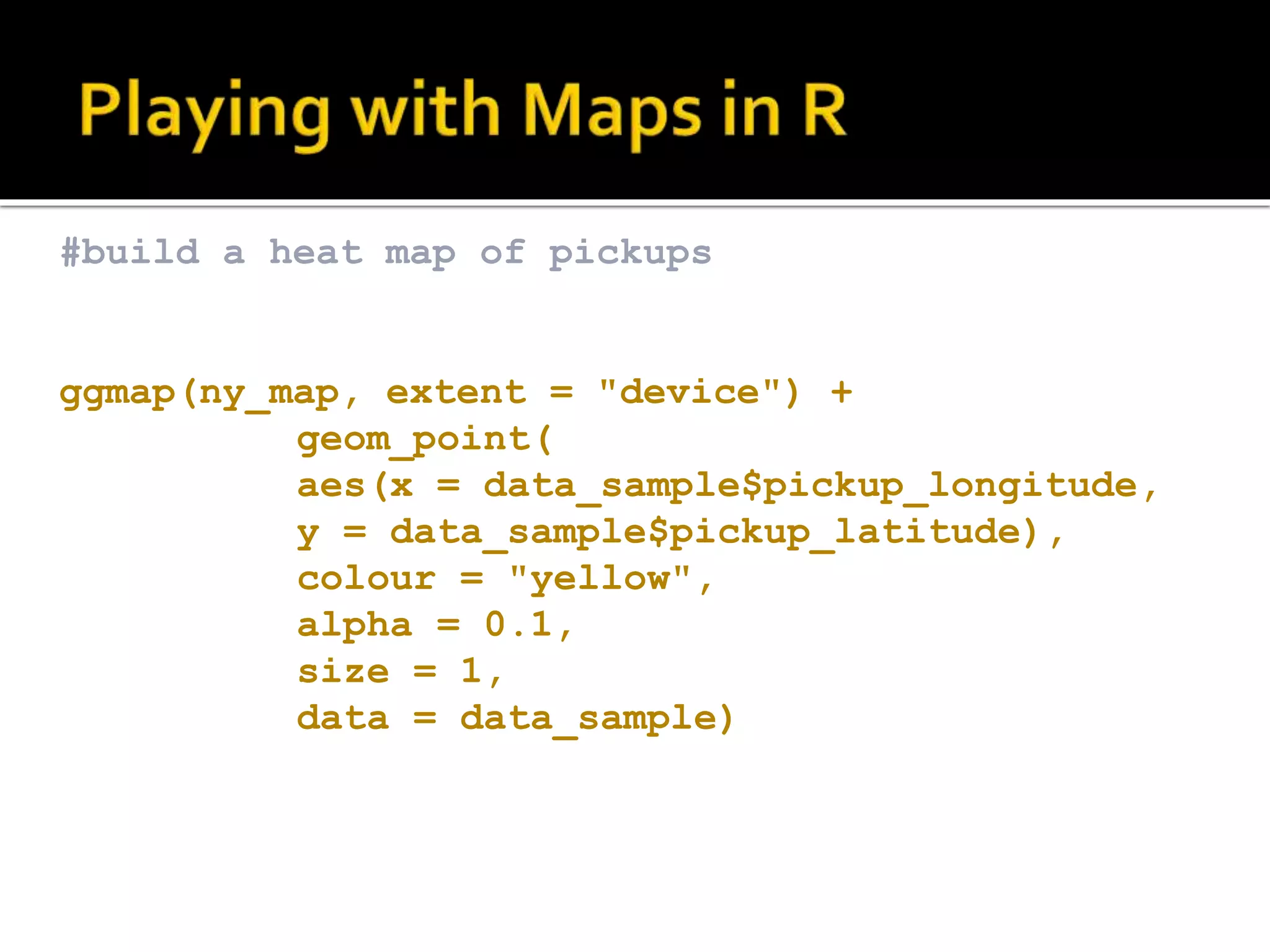
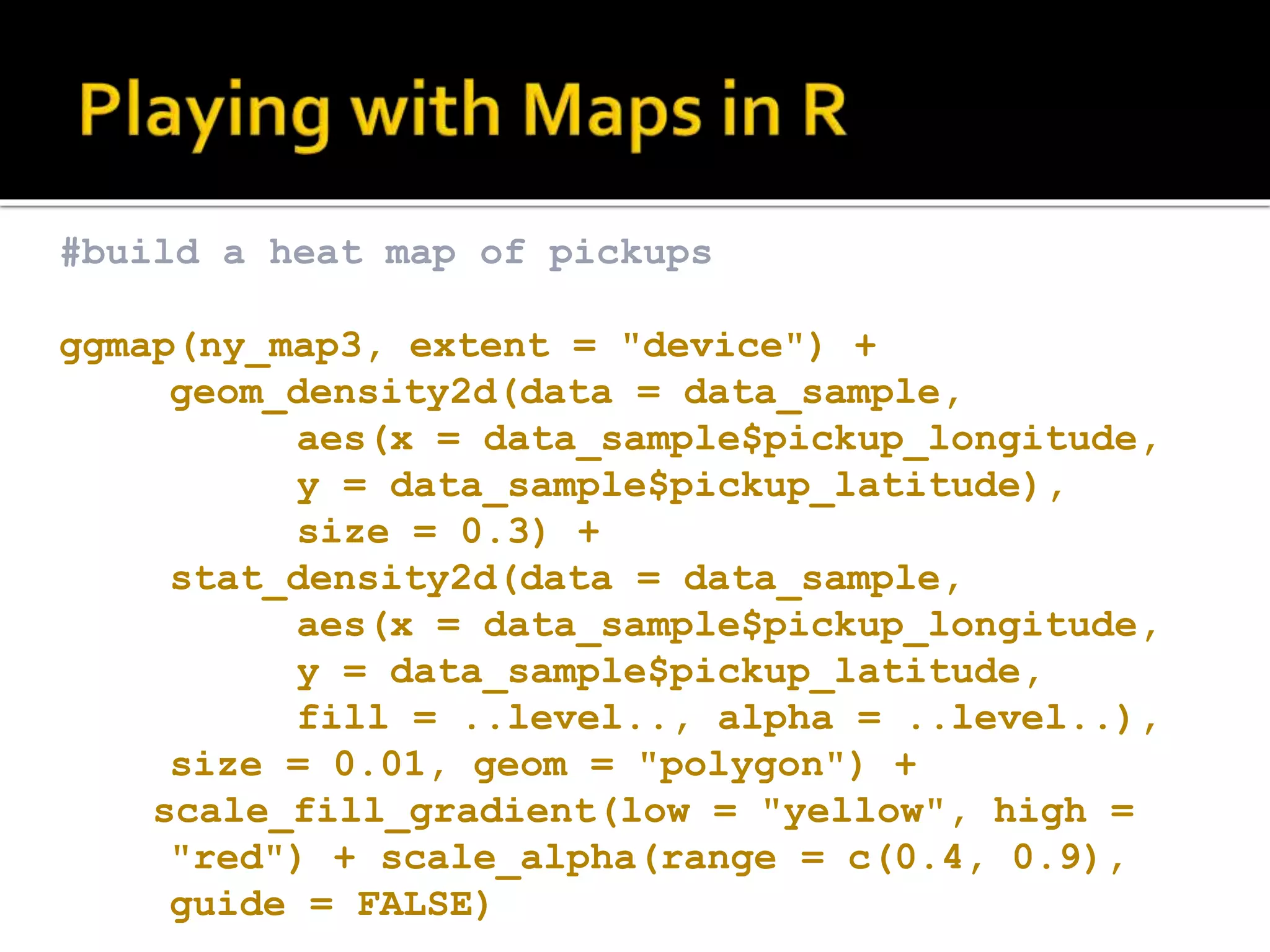
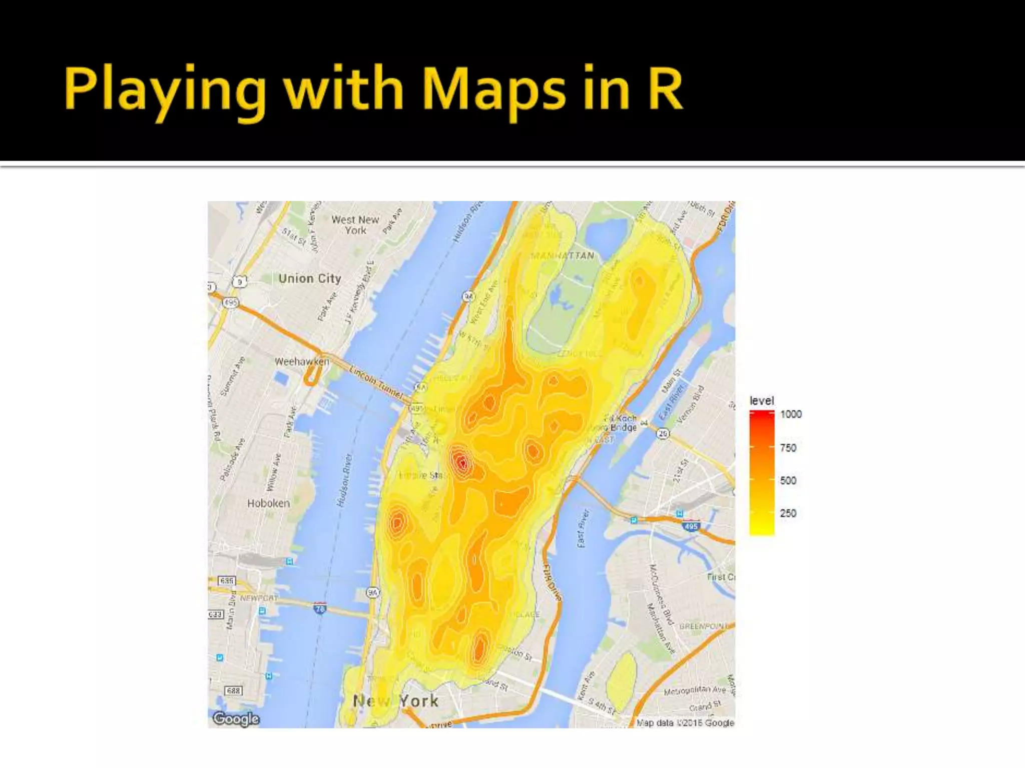
#build map for a sample of pickups data_sample<-data_trip[sample(nrow(data_trip), 400000), ] ggmap(ny_map, extent = "device") + geom_point(aes(x = data_sample$pickup_longitude, y = data_sample$pickup_latitude), colour = "yellow", alpha = 0.1, size = 1, data = data_sample)

#build a heat map of pickups ggmap(ny_map, extent = "device") + geom_point( aes(x = data_sample$pickup_longitude, y = data_sample$pickup_latitude), colour = "yellow", alpha = 0.1, size = 1, data = data_sample)

#build a heat map of pickups ggmap(ny_map3, extent = "device") + geom_density2d(data = data_sample, aes(x = data_sample$pickup_longitude, y = data_sample$pickup_latitude), size = 0.3) + stat_density2d(data = data_sample, aes(x = data_sample$pickup_longitude, y = data_sample$pickup_latitude, fill = ..level.., alpha = ..level..), size = 0.01, geom = "polygon") + scale_fill_gradient(low = "yellow", high = "red") + scale_alpha(range = c(0.4, 0.9), guide = FALSE)

+ geom_point(aes(x=top10_loc$lon,y=top10_loc$lat, size=top10_loc$counter),data=top10_loc)

#Trip with highest standard deviation of travel #time #I assume "trip" means "a taxi run with a given #trip_start and trip_end". data_trip$latdropoff<- round(data_trip$dropoff_latitude/0.005)*0.005 data_trip$slatdropoff<- lapply(data_trip$latdropoff,toString) data_trip$londropoff<- round(data_trip$dropoff_longitude/0.005)*0.005 data_trip$slondropoff<- lapply(data_trip$londropoff,toString) data_trip$trip_end<- paste(data_trip$slatdropoff,data_trip$slondropo ff,sep="|")

#get rit of not useful variables data_trip$latdropoff<-NULL data_trip$londropoff<-NULL data_trip$slatdropoff<-NULL data_trip$slondropoff<-NULL #trip_id variable data_trip$trip_id<-paste(data_trip$trip_start, data_trip$trip_end,sep="|")

#compute standard deviation for every trip trips<-aggregate(data_trip$trip_time_in_secs ~ data_trip$trip_id, data_trip, sd) #get the trip with highest standard deviation #and find pickup and dropoff locations trips.topsd<-trips %>% arrange(desc(trips[,2])) %>% top_n(10) names(trips.topsd)[names(trips.topsd)== "data_trip$trip_id"] <- "trip_id" names(trips.topsd)[names(trips.topsd)== "data_trip$trip_time_in_secs"] <- "trip_sd"

#recover from google maps and print top 10 trip by sd trip_text=list() for(i in 1:10) { coords=matrix(as.double(unlist(strsplit( trips.topsd$trip_id[i], "[|]"))), nrow=2,ncol=2,byrow=TRUE) from=coords[1,] to=coords[2,] origin<-mapply(FUN = function(lon, lat) revgeocode(c(lon, lat)), from[2], from[1]) destination<-mapply(FUN = function(lon, lat) revgeocode(c(lon, lat)), to[2], to[1]) trip_text[i]=paste("Trip",i,"from",origin,"to", destination,"has",round(trips.topsd$trip_sd[i],2), " SD.")}

print(trip_text) [[1]] [1] "Trip 1 from JFK Expressway, Jamaica, NY 11430, USA to JFK Expressway, Jamaica, NY 11430, USA has 3660.94 SD." [[2]] [1] "Trip 2 from Perimeter Rd, Jamaica, NY 11430, USA to 826 Greene Ave, Brooklyn, NY 11221, USA has 3436.54 SD." [[3]] [1] "Trip 3 from 46-36 54th Rd, Flushing, NY 11378, USA to 107-11 Van Wyck Expy, Jamaica, NY 11435, USA has 3181.98 SD.” … … [[10]] [1] "Trip 10 from Central Terminal Area, Jamaica, NY 11430, USA to 34-40 E Houston St, New York, NY 10012, USA has 2206.17 SD."

#Trip with the lowest fare’s Standard Deviation #I assume each taxy run is uniquely identified #by "hack licence" and "pickup time". #I can build unique run_id's for data_fares and #data_trip tables and join them data_fares$run_id<-paste(data_fares$hack_license, data_fares$pickup_datetime,sep="|") data_trip$run_id<-paste(data_trip$hack_license, data_trip$pickup_datetime,sep="|")

#I create a new dataframe merging data_fares and #data_trip on run_id df_merge=merge(x=data_trip,y=data_fares, by.x="run_id", by.y="run_id", all.x=TRUE) #groupby and standard deviation computation for #fare ampount fares<-aggregate(df_merge$fare_amount ~ df_merge$trip_id, df_merge, sd)

#Keep track of tot number of runs for each trip fares_c<-aggregate(df_merge$ones ~ df_merge$trip_id, df_merge, sum) fares_merge=merge(x=fares,y=fares_c, by.x="df_merge$trip_id", by.y="df_merge$trip_id", all.x=TRUE) names(fares_merge)[names(fares_merge)== "df_merge$trip_id"] <- "trip_id" names(fares_merge)[names(fares_merge)== "df_merge$fare_amount"] <- "fare_sd" names(fares_merge)[names(fares_merge)== "df_merge$ones"] <- "trip_count" #exclude trip with less then 30 runs and order fares_merge<-fares_merge[(fares_merge$trip_count>30),] fares_merge<- fares_merge %>% arrange((fares_merge$fare_sd))

#get some extra information beyond numbers trip_text=list() for(i in 1:10) { coords=matrix(as.double(unlist(strsplit( fares_merge$trip_id[i], "[|]"))), nrow=2, ncol=2,byrow=TRUE) from=coords[1,] to=coords[2,] origin<-mapply(FUN = function(lon, lat) revgeocode(c(lon, lat)), from[2], from[1]) destination<-mapply(FUN = function(lon, lat) revgeocode(c(lon, lat)), to[2], to[1]) trip_text[i]=paste("Trip",i,"starts from",origin,"and end to to",destination) }

print(trip_text) [[1]] [1] "Trip 1 starts from 1585-1589 Broadway, New York, NY 10036, USA and end to 107-11 Van Wyck Expy, Jamaica, NY 11435, USA" [[2]] [1] "Trip 2 starts from 1700 3rd Ave, New York, NY 10128, USA and end to 53 E 124th St, New York, NY 10035, USA" [[3]] [1] "Trip 3 starts from 330 W 95th St, New York, NY 10025, USA and end to 534 W 112th St, New York, NY 10025, USA" … … [[10]][1] "Trip 10 starts from 762 Amsterdam Ave, New York, NY 10025, USA and end to 192 Claremont Ave, New York, NY 10027, USA"

#prepare points to visualize nr_points=100 ffrom=matrix(nr_points*2,nrow=nr_points,ncol=2) tto=matrix(nr_points*2,nrow=nr_points,ncol=2) for(i in 1:nr_points) {coords= matrix(as.double(unlist(strsplit( fares_merge$trip_id[i], "[|]"))), nrow=2, ncol=2,byrow=TRUE) from=coords[1,] to=coords[2,] ffrom[i,1]=coords[1,1] ffrom[i,2]=coords[1,2] tto[i,1]=coords[2,1] tto[i,2]=coords[2,2] }

#transform points in a matrix to points in a dataframe start_end<-as_data_frame(list(from.lat= ffrom[,1],from.lon=ffrom[,2],to.lat=tto[,1], to.lon=tto[,2])) #plot the trip with the lowest fare’s SD ggmap(ny_map, extent = "device") + geom_point(aes(x = start_end$to.lon[1], y = start_end$to.lat[1]), colour = "red", alpha = 0.6, size = 10, data=start_end) + geom_point(aes(x = start_end$from.lon[1], y = start_end$from.lat[1]), colour = "yellow", alpha = 0.6, size = 10, data=start_end)

#plot the other trips aroung Manhattan area ggmap(ny_map3, extent = "device") + geom_point(aes(x = start_end$to.lon+0.00085, y = start_end$to.lat), colour = "red", alpha = 0.2, size = 10, data=start_end) + geom_point(aes(x = start_end$from.lon, y = start_end$from.lat),colour = "green", alpha = 0.2, size = 10, data=start_end)

Customer behaviour Economics Insights & Graphics Other Insights  We can fill our mockup now

Customer behaviour Economics Insights & Graphics Other Insights  We can fill our mockup

 Let’s use some descriptive stats instead of graph in the Customer’s Behavior Section > summary(data_trip$passenger_count) Min. 1st Qu. Median Mean 3rd Qu. Max. 1.00 1.000 1.000 2.182 3.000 6.000 > summary(data_trip$trip_time_in_secs/60) Min. 1st Qu. Median Mean 3rd Qu. Max. 1.083 6.000 10.000 11.97 15.000 128.0 > summary(data_trip$trip_distance) Min. 1st Qu. Median Mean 3rd Qu. Max. 0.110 1.160 1.930 2.943 3.420 45.46 > summary(data_fares$payment_type) CRD CSH DIS NOC UNK 257247 242503 2 16 232

 Customer Behaviour entries Average Number of Passengers p/Trip AverageTime Spent onTaxi p/Trip 2.18 12' 25th Percentile Median 75th Percentile 25th Percentile Median 75th Percentile 1 1.0 3 6' 10' 15' Average Number of Miles p/Trip PayementsType 2.94 miles Credit Card (51%) 25th Percentile Median 75th Percentile Cash NOC Other 1.2 1.9 3.4 48% 0.00% 1%

 Let’s use some descriptive statistics instead of graph in the Economics Section > summary(data_fares$fare_amount) Min. 1st Qu. Median Mean 3rd Qu. Max. 2.50 6.50 9.50 12.18 14.00 385.00 > summary(data_fares$tip_amount) Min. 1st Qu. Median Mean 3rd Qu. Max. 0.00 0.00 0.00 1.22 1.90 200.00 > summary(data_fares$total_amount) Min. 1st Qu. Median Mean 3rd Qu. Max. 2.50 8.00 11.00 14.31 16.10 490.80 > summary(data_fares$total_amount- data_fares$tip_amount-data_fares$fare_amount) Min. 1st Qu. Median Mean 3rd Qu. Max. 0.0000 0.5000 0.5000 0.9158 1.0000 20.0000

AverageTip p/Trip Average Other Earnings p/Trip 1.22 $ 0.92 $ 25th Percentile Median 75th Percentile 25th Percentile Median 75th Percentile 0 $ 0 $ 1.9 $ 0.50 $ 0.50 $ 1.00 $ AverageAmount Earned p/Trip Average Fare p/Trip 14.31 $ 12.18 $ 25th Percentile Median 75th Percentile 25th Percentile Median 75th Percentile 8.00 $ 11.00 $ 16.10 $ 6.5 $ 9.50 $ 14 $

 Include some facts from which you can infer something interesting Top 5 Busiest Hours The Busiest Hours are from 22:00 to 02:00 Trip with MostVolatileTravelTime Trip from JFK Expressway, Jamaica, NY 11430, USA to JFK Expressway, Jamaica, NY 11430, USA has 3660.94 SD. TripWith Most Consisten Fares From 1585-1589 Broadway, NY 10036 to 107-11VanWyck Expy, Jamaica, NY 11435

Customer Habits on a Taxi Trip 25th Percentile Median 75th Percentile 25th Percentile Median 75th Percentile 25th Percentile Median 75th Percentile Cash NOC Other 1 1.0 3 6' 10' 15' 1.2 1.9 3.4 48% 0.00% 1% Economics 25th Percentile Median 75th Percentile 25th Percentile Median 75th Percentile 25th Percentile Median 75th Percentile 25th Percentile Median 75th Percentile 8.00 $ 11.00 $ 16.10 $ 6.5 $ 9.50 $ 14 $ 0 $ 0 $ 1.9 $ 0.50 $ 0.50 $ 1.00 $ Taxi Life Insights Top 10 Busiest Locations Trip from JFK Expressway, Jamaica, NY 11430, USA to JFK Expressway, Jamaica, NY 11430, USA has 3660.94 SD. Trip With Most Consisten Fares From 1585-1589 Broadway, NY 10036 to 107-11 Van Wyck Expy, Jamaica, NY 11435 Pickup Points Busy Areas Top 10 Busiest Locations Top 5 Busiest Hours The Busiest Hours are from 22:00 to 02:00 Trip with Most Volatile Travel Time Average Amount Earned p/Trip Average Fare p/Trip Average Tip p/Trip Average Other Earnings p/Trip 14.31 $ 12.18 $ 1.22 $ 0.92 $ Average Number of Passengers p/Trip Average Time Spent on Taxi p/Trip Average Number of Miles p/Trip Payements Type 2.18 12' 2.94 miles Credit Card (51%) NYC Taxy Data Insigths

Using R for Building a Simple and Effective Dashboard

Using R for Building a Simple and Effective Dashboard

More Related Content

Similar to Using R for Building a Simple and Effective Dashboard

More from Andrea Gigli

Recently uploaded

Using R for Building a Simple and Effective Dashboard