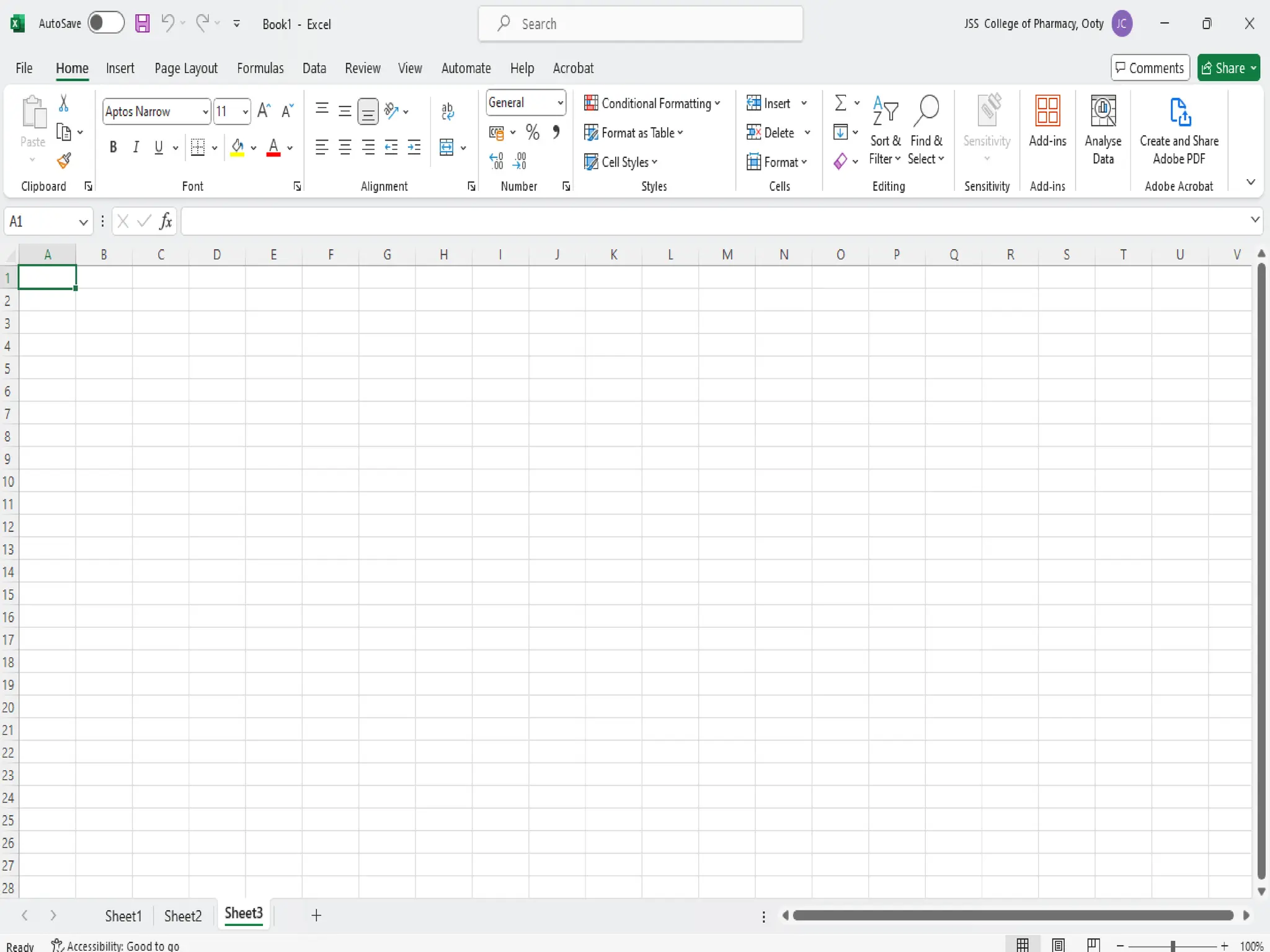
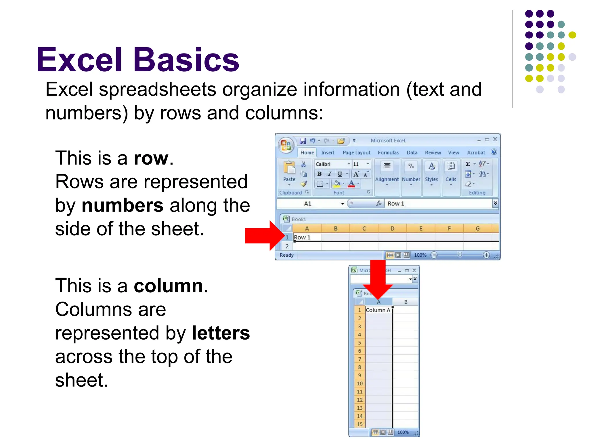
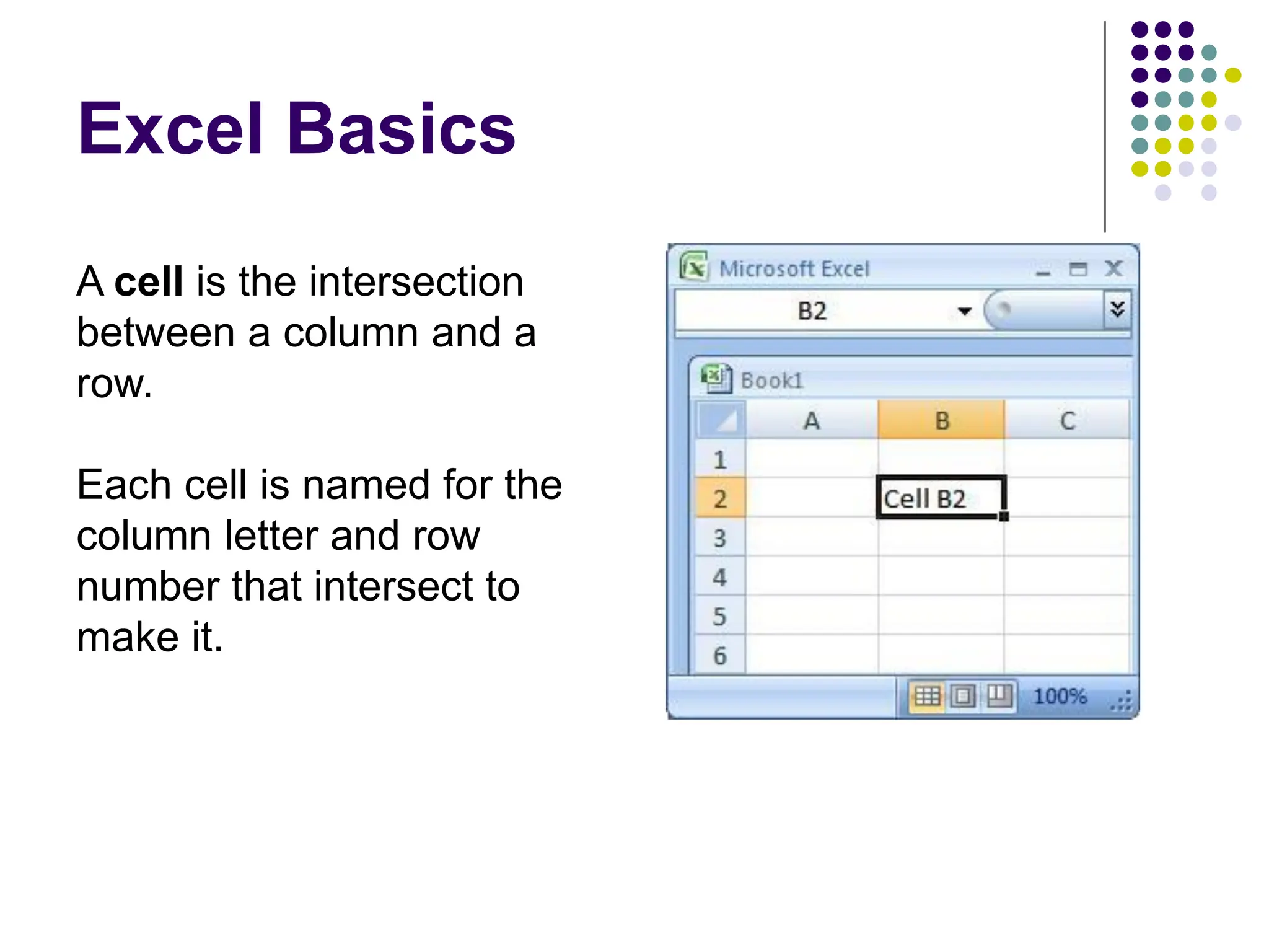
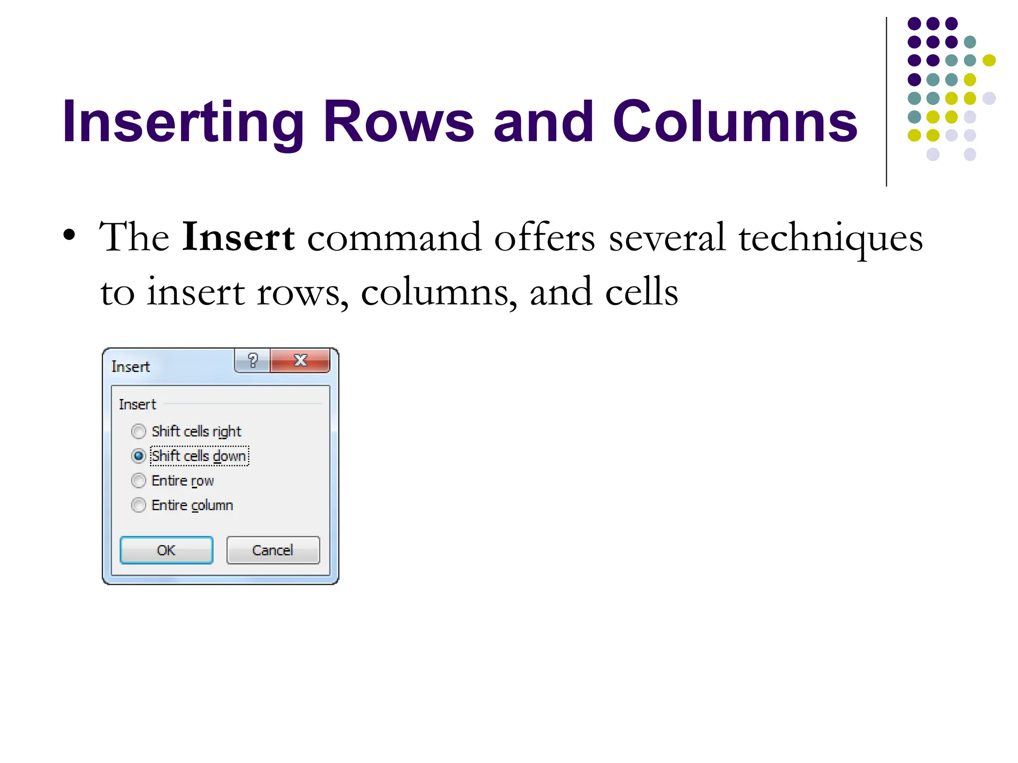
Introduction to Excel Part 1: The Basics
We will use Excel to: 1. Store and organize data, 2. Analyze data, and 3. Represent data graphically (e.g., in bar graphs, histograms, and scatterplots)
⚫ Microsoft Excel consists of Workbooks ⚫ Each Workbook is made up of an infinite number of worksheets ⚫ It is possible to name each worksheet to aid in organizing your data Excel Basics
Excel Basics This is a row. Rows are represented by numbers along the side of the sheet. This is a column. Columns are represented by letters across the top of the sheet. Excel spreadsheets organize information (text and numbers) by rows and columns:
Excel Basics A cell is the intersection between a column and a row. Each cell is named for the column letter and row number that intersect to make it.
Excel Basics ⚫ Excel allows for some basic actions which we have used before in other programs ⚫ Copy/Paste (Rows, Columns, Cells, etc.) ⚫ Insert (Rows and Columns) ⚫ Sort (Alphabetically, Numerically, Chronologically, etc.)
Inserting Rows and Columns • The Insert command offers several techniques to insert rows, columns, and cells
Deleting Rows and Columns • The Delete command offers several techniques to remove rows, columns, and cells
Formatting ⚫ Merging allows us to combine two or more adjacent cells physically (disregarding contents) ⚫ To merge cells simply highlight the cells to be merged and select the merge option from the home menu ⚫ Cells can also be formatted with options you are probably familiar with (bold, font size, borders, etc.) ⚫ These options can be found scattered on the home menu or under the format cells menu via the right-click list. Even whole rows and columns can be formatted. Let’s take a look!
Formatting ⚫ Excel also allows us to format cells by their data types. This is useful for a variety of reasons (sorting, manipulating, rounding, etc.) ⚫ To format the cell’s data type, in the numbers section of the home menu, select the number drop-down menu (defaults to General) and select the new type desired
Adjusting Column Width • Column width is the horizontal measurement of a column
Adjusting Row Height • Row height is the vertical measurement of a row – The row height is automatically adjusted with a font size increase – Using ALT+Enter to create multiple lines may require a row height adjustment – Select Row Height from the Format menu
Data Entry There are two ways to enter information into a cell: 1. Type directly into the cell. Click on a cell, and type in the data (numbers or text) and press Enter. 2. Type into the formula bar. Click on a cell, and then click in the formula bar (the space next to the ). Now type the data into the bar and press Enter.
Entering and Editing Cell Data • Excel supports text, values, dates, and formula results
Numeric Formats
Numeric Formats Continued
Data Removal ⚫ Data can be removed from a cell, column, or row easily ⚫ Here are a few methods: ⚫ Click the column or row heading that you want deleted, then click the Delete in the Cells group on the Home tab ⚫ Another method for entire row/column deletion is to click a cell in the row or column and follow the above method respectively ⚫ Delete methods are also found via the right-click menu ⚫ To remove data from a cell or group of cells, simply highlight those to be deleted and press delete
• A range is a rectangular group of cells • A nonadjacent range contains a group of ranges that are not next to each other Selecting a Cell Range
Auto Fill ⚫ Auto Fill enables us to copy the contents of a cell or a range of cells by dragging the fill handle over adjacent cells or a range ⚫ To use Auto Fill: ⚫ 1. Click the cell with the content you want to copy to make it the active cell ⚫ 2. Position the pointer over the bottom-right corner of the cell until it changes to the fill pointer (a thin black plus sign) ⚫ 3. Drag the fill handle to repeat the content in other cells
Formulas and Functions ⚫ Formulas are equations that perform calculations in your spreadsheet. Formulas always begin with an equals sign (=). When you enter an equals sign into a cell, you are basically telling Excel to “calculate this.” ⚫ Functions are Excel-defined formulas. They take data you select and enter, perform calculations on them, and return value(s).
Mathematical Symbols
Order of Precedence • Order of precedence (operations) controls the sequence in which math operators are computed – Parentheses – Exponentiation – Multiplication and Division – Addition and Subtraction
Cell References in Formulas • It is best to use cell addresses in formulas versus actual data – If cell A1 contains value 5 and you need to add B1 to this value, use =A1+B1 versus =5+B1 • If the data changes, Excel will recalculate the result
Functions ⚫ All functions have a common format – the equals sign followed by the function name followed by the input in parentheses. ⚫ The input for a function can be either: ⚫ A set of numbers (e.g., “=AVERAGE(2, 3, 4, 5)”) ⚫ This tells Excel to calculate the average of these numbers. ⚫ A reference to cell(s) (e.g., “=AVERAGE(B1:B18) or “=AVERAGE (B1, B2, B3, B4, B5, B6, B7, B8)” ⚫ This tells Excel to calculate the average of the data that appear in all the cells from B1 to B8. ⚫ You can either type these cell references in by hand or by clicking and dragging with your mouse to select the cells.
Functions for Descriptive Statistics =AVERAGE(first cell:last cell): calculates the mean =MEDIAN(first cell:last cell): calculates the median =MODE(first cell:last cell): calculates the mode =VARP(first cell:last cell): calculates the variance =STDEVP(first cell:last cell): calculates the standard deviation ⚫ You may directly write the functions for these statistics into cells or the formula bar, OR ⚫ You may use the function wizard ( in the toolbar) Below are several functions you may need to learn for this class.
28 To Set Up Statistical Package ⚫ Click File Tab, and Then Click Options. ⚫ Click Add-ins. In View and Manage Box, Select Analysis ToolPak. ⚫ Click Go. ⚫ In the Add-Ins Available Box, Select Analysis ToolPak Check Box and Click OK. (If ToolPak Is Not Listed, Click Browse to Locate It.)
29 Using Excel: Descriptive Statistics ⚫ Click Data/Data Analysis (Far Right) /Descriptive Statistics & OK. ⚫ Put Checkmarks on Summary Statistics, 95% or 99% Confidence Interval, & Labels in First Row Boxes. ⚫ Move Cursor to Input Range Window, Highlight Data to Analyze including Labels, & Click OK. ⚫ Your Data will Appear on New Worksheet. ⚫ Widen Columns by Clicking Home/Format/AutoFit Column Width.
30 Using Excel: Constructing Histograms ⚫ Click Data/Data Analysis/Histogram & OK. ⚫ Put Checkmarks on Chart Output & New Worksheet Boxes. ⚫ Move Cursor to Input Range Window, Highlight Data Going into Histogram. ⚫ Move Cursor to Input Bin Range, Highlight Data Showing Upper Value of Each Bin & Click OK. ⚫ Histogram will be on New Worksheet. You May Lengthen it by Clicking Blank Space in Window, Moving Cursor to Window Bottom Line & Holding Down Mouse Button as You Pull Down Window.
31 Using Excel: Hypothesis Testing ⚫ Go to Sheet One. ⚫ Click Data/Data Analysis/ and the Appropriate Statistical Test. Then Click OK. ⚫ On New Window Check Labels Box and Put Cursor on Variable 1 Range. ⚫ Highlight Variable 1 Data Including Label. ⚫ Put Cursor on Variable 2 Range & Highlight Variable 2 Data (Including Label). Then Click OK. ⚫ Click Home/Format/AutoFit/Column Width
32 Using Excel: Scatter Plots ⚫ Go to Sheet One. ⚫ Highlight Data (Be Sure X Values are in Left Column and Y Values are in Right Column). ⚫ Click Insert/Scatter. Pull down menu and click Upper Left Icon. ⚫ Click a Datum Point on Chart with Right Mouse Key, Add Trendline, & Click Linear.
33 Using Excel: Regression Analysis ⚫ Go to Sheet One. ⚫ Click Data/Data Analysis (On Far Right) /Regression & Click OK. ⚫ On New Window Check Labels Box and Put Cursor on X Range. ⚫ Highlight X Data Including Label. ⚫ Put Cursor on Y Range & Highlight Y Data (Including Label), Then Click OK. ⚫ Click Home/Format/AutoFit Column Width.

Using procedure of excel and methods to use they way and design

  • 1.
  • 2.
    We will useExcel to: 1. Store and organize data, 2. Analyze data, and 3. Represent data graphically (e.g., in bar graphs, histograms, and scatterplots)
  • 3.
    ⚫ Microsoft Excelconsists of Workbooks ⚫ Each Workbook is made up of an infinite number of worksheets ⚫ It is possible to name each worksheet to aid in organizing your data Excel Basics
  • 5.
    Excel Basics This isa row. Rows are represented by numbers along the side of the sheet. This is a column. Columns are represented by letters across the top of the sheet. Excel spreadsheets organize information (text and numbers) by rows and columns:
  • 6.
    Excel Basics A cellis the intersection between a column and a row. Each cell is named for the column letter and row number that intersect to make it.
  • 7.
    Excel Basics ⚫ Excelallows for some basic actions which we have used before in other programs ⚫ Copy/Paste (Rows, Columns, Cells, etc.) ⚫ Insert (Rows and Columns) ⚫ Sort (Alphabetically, Numerically, Chronologically, etc.)
  • 8.
    Inserting Rows andColumns • The Insert command offers several techniques to insert rows, columns, and cells
  • 9.
    Deleting Rows andColumns • The Delete command offers several techniques to remove rows, columns, and cells
  • 10.
    Formatting ⚫ Merging allowsus to combine two or more adjacent cells physically (disregarding contents) ⚫ To merge cells simply highlight the cells to be merged and select the merge option from the home menu ⚫ Cells can also be formatted with options you are probably familiar with (bold, font size, borders, etc.) ⚫ These options can be found scattered on the home menu or under the format cells menu via the right-click list. Even whole rows and columns can be formatted. Let’s take a look!
  • 11.
    Formatting ⚫ Excel alsoallows us to format cells by their data types. This is useful for a variety of reasons (sorting, manipulating, rounding, etc.) ⚫ To format the cell’s data type, in the numbers section of the home menu, select the number drop-down menu (defaults to General) and select the new type desired
  • 12.
    Adjusting Column Width •Column width is the horizontal measurement of a column
  • 13.
    Adjusting Row Height •Row height is the vertical measurement of a row – The row height is automatically adjusted with a font size increase – Using ALT+Enter to create multiple lines may require a row height adjustment – Select Row Height from the Format menu
  • 14.
    Data Entry There aretwo ways to enter information into a cell: 1. Type directly into the cell. Click on a cell, and type in the data (numbers or text) and press Enter. 2. Type into the formula bar. Click on a cell, and then click in the formula bar (the space next to the ). Now type the data into the bar and press Enter.
  • 15.
    Entering and EditingCell Data • Excel supports text, values, dates, and formula results
  • 16.
  • 17.
  • 18.
  • 19.
    Data Removal ⚫ Datacan be removed from a cell, column, or row easily ⚫ Here are a few methods: ⚫ Click the column or row heading that you want deleted, then click the Delete in the Cells group on the Home tab ⚫ Another method for entire row/column deletion is to click a cell in the row or column and follow the above method respectively ⚫ Delete methods are also found via the right-click menu ⚫ To remove data from a cell or group of cells, simply highlight those to be deleted and press delete
  • 20.
    • A rangeis a rectangular group of cells • A nonadjacent range contains a group of ranges that are not next to each other Selecting a Cell Range
  • 21.
    Auto Fill ⚫ AutoFill enables us to copy the contents of a cell or a range of cells by dragging the fill handle over adjacent cells or a range ⚫ To use Auto Fill: ⚫ 1. Click the cell with the content you want to copy to make it the active cell ⚫ 2. Position the pointer over the bottom-right corner of the cell until it changes to the fill pointer (a thin black plus sign) ⚫ 3. Drag the fill handle to repeat the content in other cells
  • 22.
    Formulas and Functions ⚫Formulas are equations that perform calculations in your spreadsheet. Formulas always begin with an equals sign (=). When you enter an equals sign into a cell, you are basically telling Excel to “calculate this.” ⚫ Functions are Excel-defined formulas. They take data you select and enter, perform calculations on them, and return value(s).
  • 23.
  • 24.
    Order of Precedence •Order of precedence (operations) controls the sequence in which math operators are computed – Parentheses – Exponentiation – Multiplication and Division – Addition and Subtraction
  • 25.
    Cell References inFormulas • It is best to use cell addresses in formulas versus actual data – If cell A1 contains value 5 and you need to add B1 to this value, use =A1+B1 versus =5+B1 • If the data changes, Excel will recalculate the result
  • 26.
    Functions ⚫ All functionshave a common format – the equals sign followed by the function name followed by the input in parentheses. ⚫ The input for a function can be either: ⚫ A set of numbers (e.g., “=AVERAGE(2, 3, 4, 5)”) ⚫ This tells Excel to calculate the average of these numbers. ⚫ A reference to cell(s) (e.g., “=AVERAGE(B1:B18) or “=AVERAGE (B1, B2, B3, B4, B5, B6, B7, B8)” ⚫ This tells Excel to calculate the average of the data that appear in all the cells from B1 to B8. ⚫ You can either type these cell references in by hand or by clicking and dragging with your mouse to select the cells.
  • 27.
    Functions for DescriptiveStatistics =AVERAGE(first cell:last cell): calculates the mean =MEDIAN(first cell:last cell): calculates the median =MODE(first cell:last cell): calculates the mode =VARP(first cell:last cell): calculates the variance =STDEVP(first cell:last cell): calculates the standard deviation ⚫ You may directly write the functions for these statistics into cells or the formula bar, OR ⚫ You may use the function wizard ( in the toolbar) Below are several functions you may need to learn for this class.
  • 28.
    28 To Set UpStatistical Package ⚫ Click File Tab, and Then Click Options. ⚫ Click Add-ins. In View and Manage Box, Select Analysis ToolPak. ⚫ Click Go. ⚫ In the Add-Ins Available Box, Select Analysis ToolPak Check Box and Click OK. (If ToolPak Is Not Listed, Click Browse to Locate It.)
  • 29.
    29 Using Excel: Descriptive Statistics ⚫Click Data/Data Analysis (Far Right) /Descriptive Statistics & OK. ⚫ Put Checkmarks on Summary Statistics, 95% or 99% Confidence Interval, & Labels in First Row Boxes. ⚫ Move Cursor to Input Range Window, Highlight Data to Analyze including Labels, & Click OK. ⚫ Your Data will Appear on New Worksheet. ⚫ Widen Columns by Clicking Home/Format/AutoFit Column Width.
  • 30.
    30 Using Excel: Constructing Histograms ⚫Click Data/Data Analysis/Histogram & OK. ⚫ Put Checkmarks on Chart Output & New Worksheet Boxes. ⚫ Move Cursor to Input Range Window, Highlight Data Going into Histogram. ⚫ Move Cursor to Input Bin Range, Highlight Data Showing Upper Value of Each Bin & Click OK. ⚫ Histogram will be on New Worksheet. You May Lengthen it by Clicking Blank Space in Window, Moving Cursor to Window Bottom Line & Holding Down Mouse Button as You Pull Down Window.
  • 31.
    31 Using Excel: Hypothesis Testing ⚫Go to Sheet One. ⚫ Click Data/Data Analysis/ and the Appropriate Statistical Test. Then Click OK. ⚫ On New Window Check Labels Box and Put Cursor on Variable 1 Range. ⚫ Highlight Variable 1 Data Including Label. ⚫ Put Cursor on Variable 2 Range & Highlight Variable 2 Data (Including Label). Then Click OK. ⚫ Click Home/Format/AutoFit/Column Width
  • 32.
    32 Using Excel: Scatter Plots ⚫Go to Sheet One. ⚫ Highlight Data (Be Sure X Values are in Left Column and Y Values are in Right Column). ⚫ Click Insert/Scatter. Pull down menu and click Upper Left Icon. ⚫ Click a Datum Point on Chart with Right Mouse Key, Add Trendline, & Click Linear.
  • 33.
    33 Using Excel: Regression Analysis ⚫Go to Sheet One. ⚫ Click Data/Data Analysis (On Far Right) /Regression & Click OK. ⚫ On New Window Check Labels Box and Put Cursor on X Range. ⚫ Highlight X Data Including Label. ⚫ Put Cursor on Y Range & Highlight Y Data (Including Label), Then Click OK. ⚫ Click Home/Format/AutoFit Column Width.