Greedy Method • "GreedyMethod finds out of many options, but you have to choose the best option.“ • Greedy Algorithm solves problems by making the best choice that seems best at the particular moment. Many optimization problems can be determined using a greedy algorithm. Some issues have no efficient solution, but a greedy algorithm may provide a solution that is close to optimal. A greedy algorithm works if a problem exhibits the following two properties: • Greedy Choice Property: A globally optimal solution can be reached at by creating a locally optimal solution. In other words, an optimal solution can be obtained by creating "greedy" choices. • Optimal substructure: Optimal solutions contain optimal subsolutions. In other words, answers to subproblems of an optimal solution are optimal. 10-02-2021 18CSC205J Operating Systems- Memory Management 4
5.
Greedy Method (Cont.) Stepsfor achieving a Greedy Algorithm are: •Feasible: Here we check whether it satisfies all possible constraints or not, to obtain at least one solution to our problems. •Local Optimal Choice: In this, the choice should be the optimum which is selected from the currently available •Unalterable: Once the decision is made, at any subsequence step that option is not altered. 10-02-2021 18CSC205J Operating Systems- Memory Management 5
6.
Greedy Method (Cont.) Example: •Machinescheduling •Fractional Knapsack Problem •Minimum Spanning Tree •Huffman Code •Job Sequencing •Activity Selection Problem 10-02-2021 18CSC205J Operating Systems- Memory Management 6
Dynamic Programming •Dynamic Programmingis the most powerful design technique for solving optimization problems. •Divide & Conquer algorithm partition the problem into disjoint sub-problems solve the sub-problems recursively and then combine their solution to solve the original problems. •Dynamic Programming is used when the subproblems are not independent, e.g. when they share the same subproblems. In this case, divide and conquer may do more work than necessary, because it solves the same sub problem multiple times. 10-02-2021 18CSC205J Operating Systems- Memory Management 8
9.
Dynamic Programming (Cont.) •DynamicProgramming solves each subproblems just once and stores the result in a table so that it can be repeatedly retrieved if needed again. •Dynamic Programming is a Bottom-up approach- we solve all possible small problems and then combine to obtain solutions for bigger problems. •Dynamic Programming is a paradigm of algorithm design in which an optimization problem is solved by a combination of achieving sub-problem solutions and appearing to the "principle of optimality". 10-02-2021 18CSC205J Operating Systems- Memory Management 9
10.
Characteristics of DynamicProgramming Dynamic Programming works when a problem has the following features:- •Optimal Substructure: If an optimal solution contains optimal sub solutions then a problem exhibits optimal substructure. •Overlapping sub-problems: When a recursive algorithm would visit the same sub-problems repeatedly, then a problem has overlapping sub-problems. 10-02-2021 18CSC205J Operating Systems- Memory Management 10
11.
Characteristics of DynamicProgramming •If a problem has optimal substructure, then we can recursively define an optimal solution. If a problem has overlapping sub-problems, then we can improve on a recursive implementation by computing each sub-problem only once. •If a problem doesn't have optimal substructure, there is no basis for defining a recursive algorithm to find the optimal solutions. If a problem doesn't have overlapping sub problems, we don't have anything to gain by using dynamic programming. •If the space of sub-problems is enough (i.e. polynomial in the size of the input), dynamic programming can be much more efficient than recursion. 10-02-2021 18CSC205J Operating Systems- Memory Management 11
12.
Elements of DynamicProgramming • Substructure: Decompose the given problem into smaller sub-problems. Express the solution of the original problem in terms of the solution for smaller problems. • Table Structure: After solving the sub-problems, store the results to the sub problems in a table. This is done because sub-problem solutions are reused many times, and we do not want to repeatedly solve the same problem over and over again. • Bottom-up Computation: Using table, combine the solution of smaller sub-problems to solve larger sub-problems and eventually arrives at a solution to complete problem. Note: Bottom-up means:- • Start with smallest sub-problems. • Combining their solutions obtain the solution to sub-problems of increasing size. • Until solving at the solution of the original problem. 10-02-2021 18CSC205J Operating Systems- Memory Management 12
13.
Components of DynamicProgramming 1. Stages: The problem can be divided into several sub-problems, which are called stages. A stage is a small portion of a given problem. For example, in the shortest path problem, they were defined by the structure of the graph. 2. States: Each stage has several states associated with it. The states for the shortest path problem was the node reached. 3. Decision: At each stage, there can be multiple choices out of which one of the best decisions should be taken. The decision taken at every stage should be optimal; this is called a stage decision. 4. Optimal policy: It is a rule which determines the decision at each stage; a policy is called an optimal policy if it is globally optimal. This is known as Bellman principle of optimality. 5. Given the current state, the optimal choices for each of the remaining states does not depend on the previous states or decisions. In the shortest path problem, it was not necessary to know how we got a node only that we did. 6. There exist a recursive relationship that identify the optimal decisions for stage j, given that stage j+1, has already been solved. 7. The final stage must be solved by itself. 10-02-2021 18CSC205J Operating Systems- Memory Management 13
14.
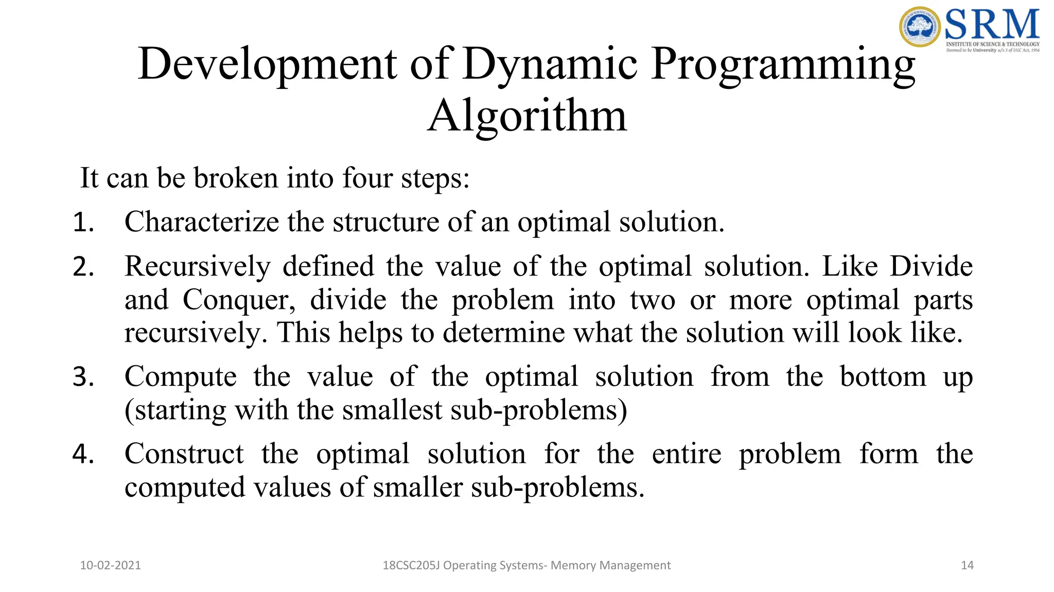
Development of DynamicProgramming Algorithm It can be broken into four steps: 1. Characterize the structure of an optimal solution. 2. Recursively defined the value of the optimal solution. Like Divide and Conquer, divide the problem into two or more optimal parts recursively. This helps to determine what the solution will look like. 3. Compute the value of the optimal solution from the bottom up (starting with the smallest sub-problems) 4. Construct the optimal solution for the entire problem form the computed values of smaller sub-problems. 10-02-2021 18CSC205J Operating Systems- Memory Management 14
15.
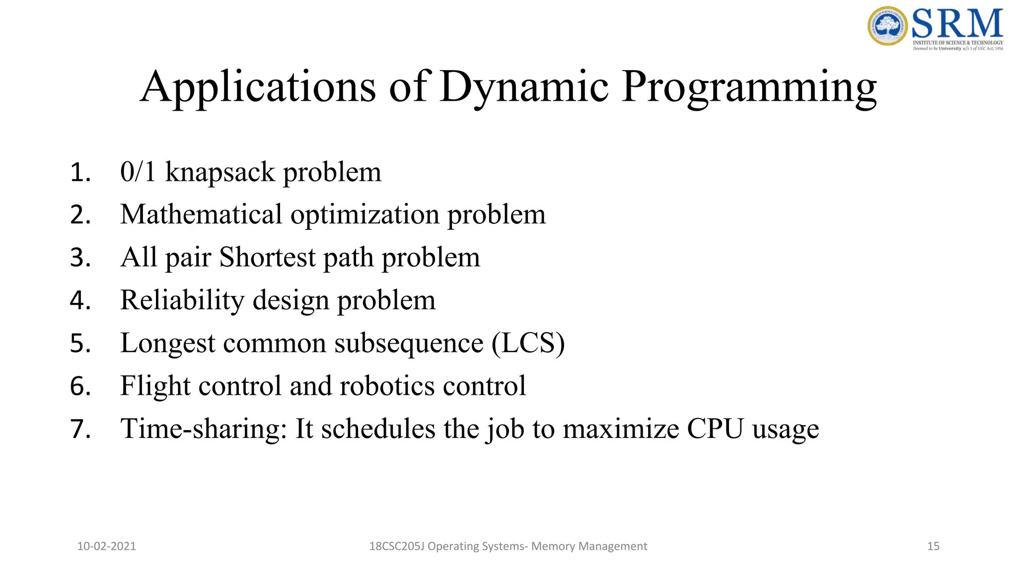
Applications of DynamicProgramming 1. 0/1 knapsack problem 2. Mathematical optimization problem 3. All pair Shortest path problem 4. Reliability design problem 5. Longest common subsequence (LCS) 6. Flight control and robotics control 7. Time-sharing: It schedules the job to maximize CPU usage 10-02-2021 18CSC205J Operating Systems- Memory Management 15
16.
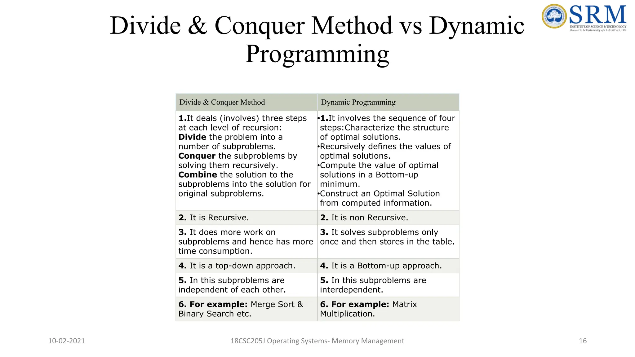
Divide & ConquerMethod vs Dynamic Programming Divide & Conquer Method Dynamic Programming 1.It deals (involves) three steps at each level of recursion: Divide the problem into a number of subproblems. Conquer the subproblems by solving them recursively. Combine the solution to the subproblems into the solution for original subproblems. •1.It involves the sequence of four steps:Characterize the structure of optimal solutions. •Recursively defines the values of optimal solutions. •Compute the value of optimal solutions in a Bottom-up minimum. •Construct an Optimal Solution from computed information. 2. It is Recursive. 2. It is non Recursive. 3. It does more work on subproblems and hence has more time consumption. 3. It solves subproblems only once and then stores in the table. 4. It is a top-down approach. 4. It is a Bottom-up approach. 5. In this subproblems are independent of each other. 5. In this subproblems are interdependent. 6. For example: Merge Sort & Binary Search etc. 6. For example: Matrix Multiplication. 10-02-2021 18CSC205J Operating Systems- Memory Management 16
17.
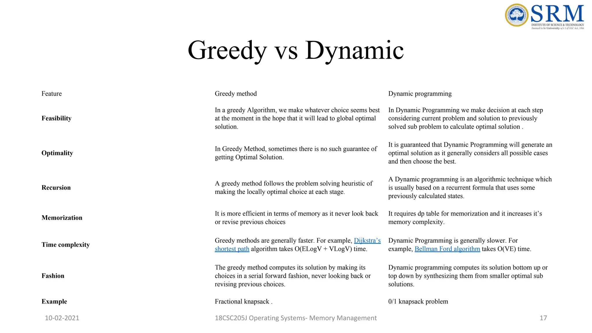
Greedy vs Dynamic FeatureGreedy method Dynamic programming Feasibility In a greedy Algorithm, we make whatever choice seems best at the moment in the hope that it will lead to global optimal solution. In Dynamic Programming we make decision at each step considering current problem and solution to previously solved sub problem to calculate optimal solution . Optimality In Greedy Method, sometimes there is no such guarantee of getting Optimal Solution. It is guaranteed that Dynamic Programming will generate an optimal solution as it generally considers all possible cases and then choose the best. Recursion A greedy method follows the problem solving heuristic of making the locally optimal choice at each stage. A Dynamic programming is an algorithmic technique which is usually based on a recurrent formula that uses some previously calculated states. Memorization It is more efficient in terms of memory as it never look back or revise previous choices It requires dp table for memorization and it increases it’s memory complexity. Time complexity Greedy methods are generally faster. For example, Dijkstra’s shortest path algorithm takes O(ELogV + VLogV) time. Dynamic Programming is generally slower. For example, Bellman Ford algorithm takes O(VE) time. Fashion The greedy method computes its solution by making its choices in a serial forward fashion, never looking back or revising previous choices. Dynamic programming computes its solution bottom up or top down by synthesizing them from smaller optimal sub solutions. Example Fractional knapsack . 0/1 knapsack problem 10-02-2021 18CSC205J Operating Systems- Memory Management 17
18.
Course Learning Outcome: Apply Greedy approach to solve Huffman coding Comparison of Brute force and Huffman method of Encoding
19.
Topics •Huffman Problem •Problem Analysis(Real Time Example) •Binary coding techniques •Prefix codes •Algorithm of Huffman Coding Problem •Time Complexity •Analysis and Greedy Algorithm •Conclusion
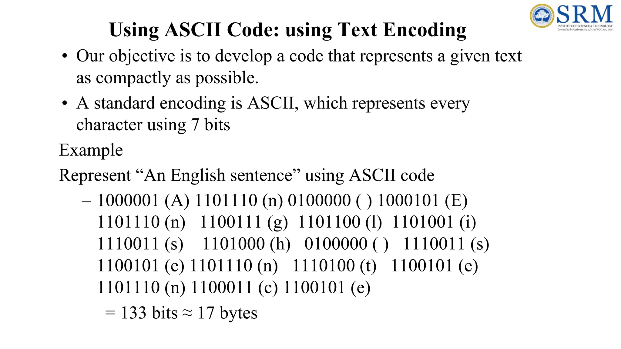
• Our objectiveis to develop a code that represents a given text as compactly as possible. • A standard encoding is ASCII, which represents every character using 7 bits Example Represent “An English sentence” using ASCII code – 1000001 (A) 1101110 (n) 0100000 ( ) 1000101 (E) 1101110 (n) 1100111 (g) 1101100 (l) 1101001 (i) 1110011 (s) 1101000 (h) 0100000 ( ) 1110011 (s) 1100101 (e) 1101110 (n) 1110100 (t) 1100101 (e) 1101110 (n) 1100011 (c) 1100101 (e) = 133 bits ≈ 17 bytes Using ASCII Code: using Text Encoding
22.
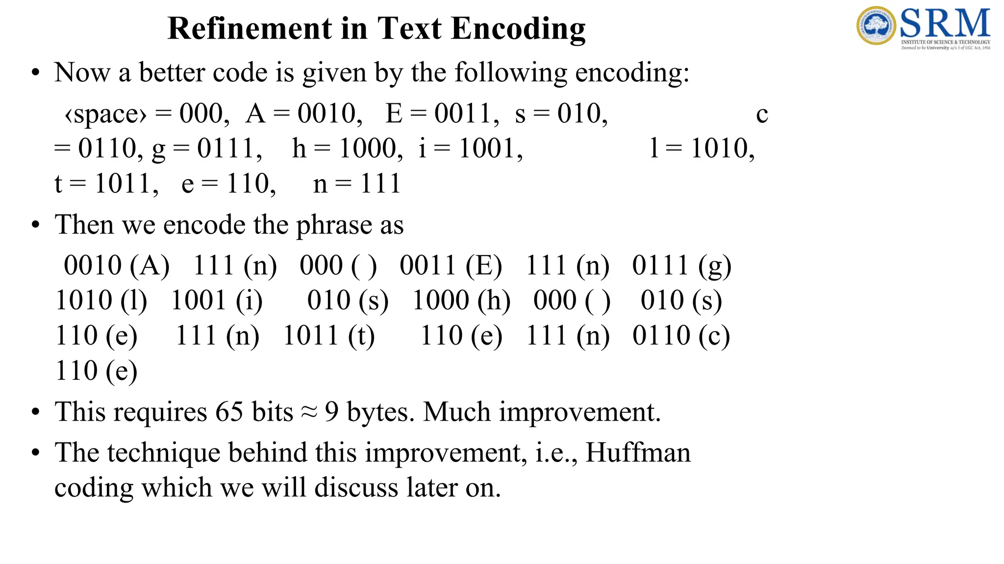
Refinement in TextEncoding • Now a better code is given by the following encoding: ‹space› = 000, A = 0010, E = 0011, s = 010, c = 0110, g = 0111, h = 1000, i = 1001, l = 1010, t = 1011, e = 110, n = 111 • Then we encode the phrase as 0010 (A) 111 (n) 000 ( ) 0011 (E) 111 (n) 0111 (g) 1010 (l) 1001 (i) 010 (s) 1000 (h) 000 ( ) 010 (s) 110 (e) 111 (n) 1011 (t) 110 (e) 111 (n) 0110 (c) 110 (e) • This requires 65 bits ≈ 9 bytes. Much improvement. • The technique behind this improvement, i.e., Huffman coding which we will discuss later on.
23.
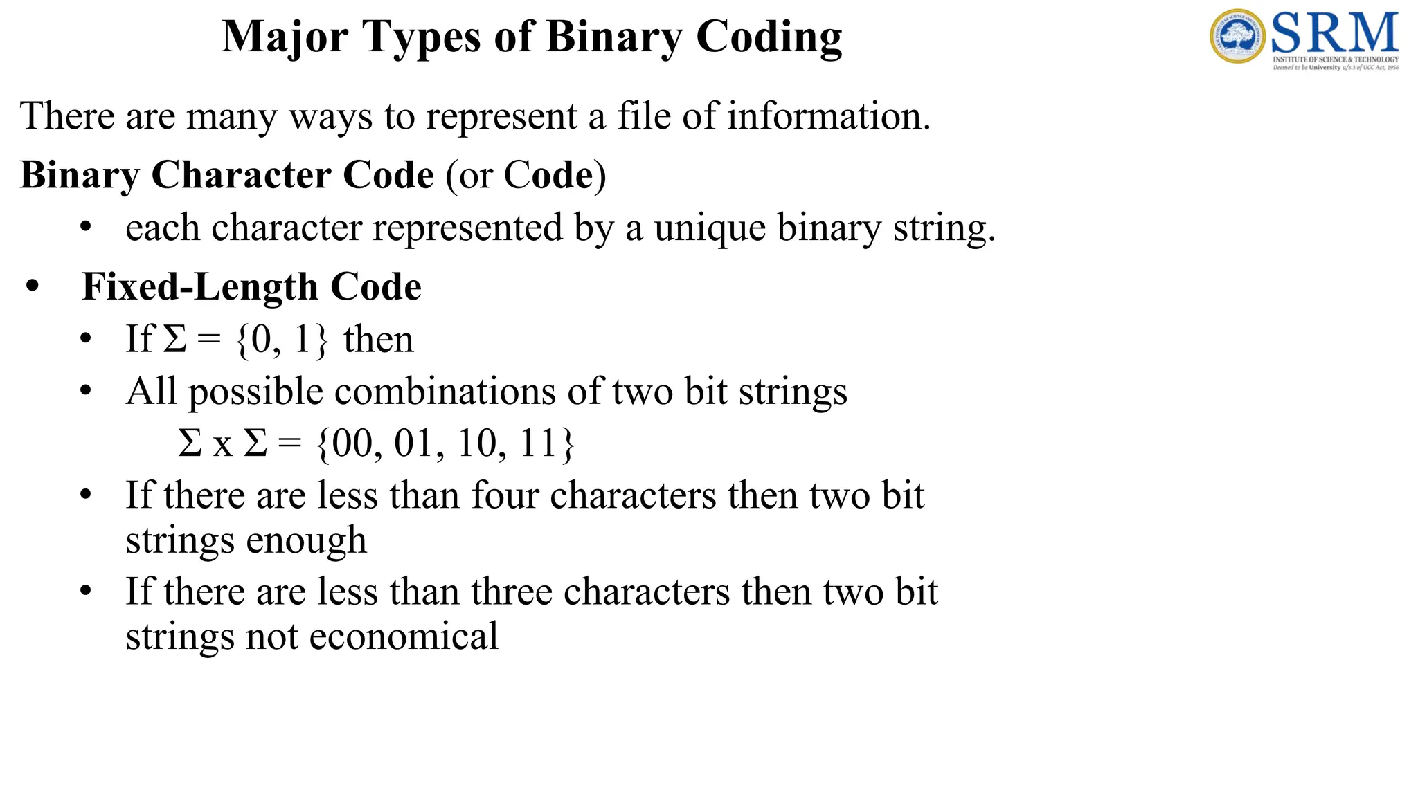
There are manyways to represent a file of information. Binary Character Code (or Code) • each character represented by a unique binary string. • Fixed-Length Code • If Σ = {0, 1} then • All possible combinations of two bit strings Σ x Σ = {00, 01, 10, 11} • If there are less than four characters then two bit strings enough • If there are less than three characters then two bit strings not economical Major Types of Binary Coding
24.
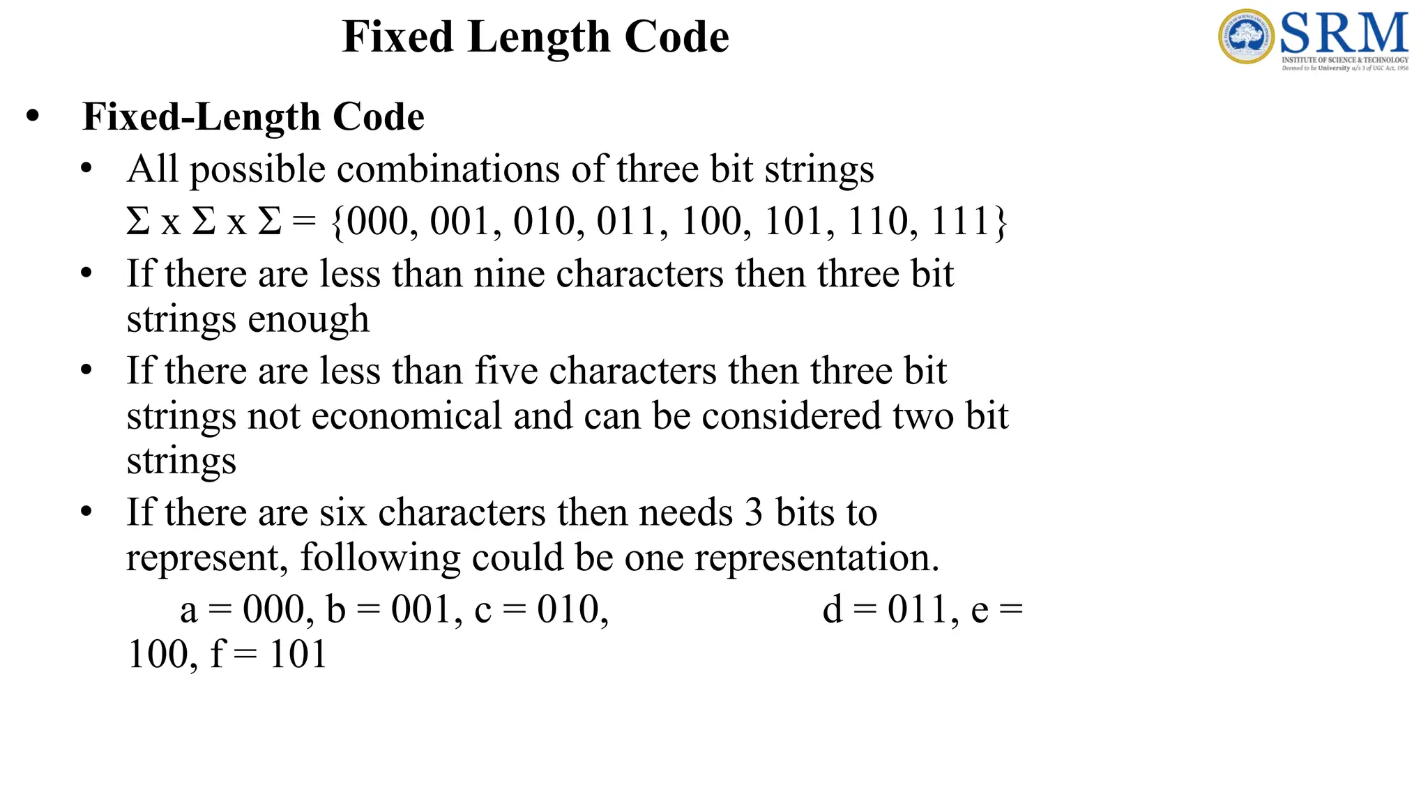
• Fixed-Length Code •All possible combinations of three bit strings Σ x Σ x Σ = {000, 001, 010, 011, 100, 101, 110, 111} • If there are less than nine characters then three bit strings enough • If there are less than five characters then three bit strings not economical and can be considered two bit strings • If there are six characters then needs 3 bits to represent, following could be one representation. a = 000, b = 001, c = 010, d = 011, e = 100, f = 101 Fixed Length Code
25.
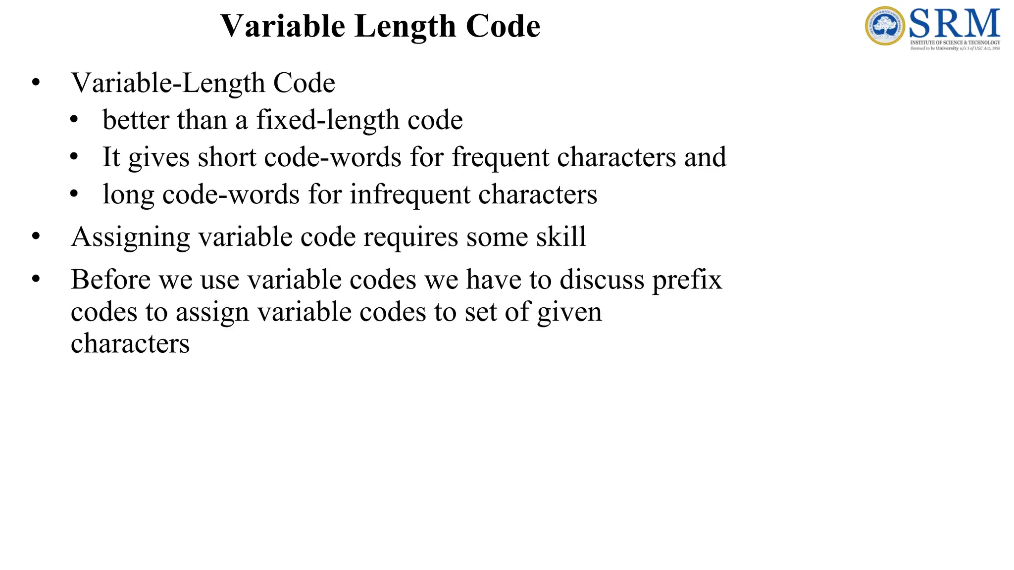
• Variable-Length Code •better than a fixed-length code • It gives short code-words for frequent characters and • long code-words for infrequent characters • Assigning variable code requires some skill • Before we use variable codes we have to discuss prefix codes to assign variable codes to set of given characters Variable Length Code
26.
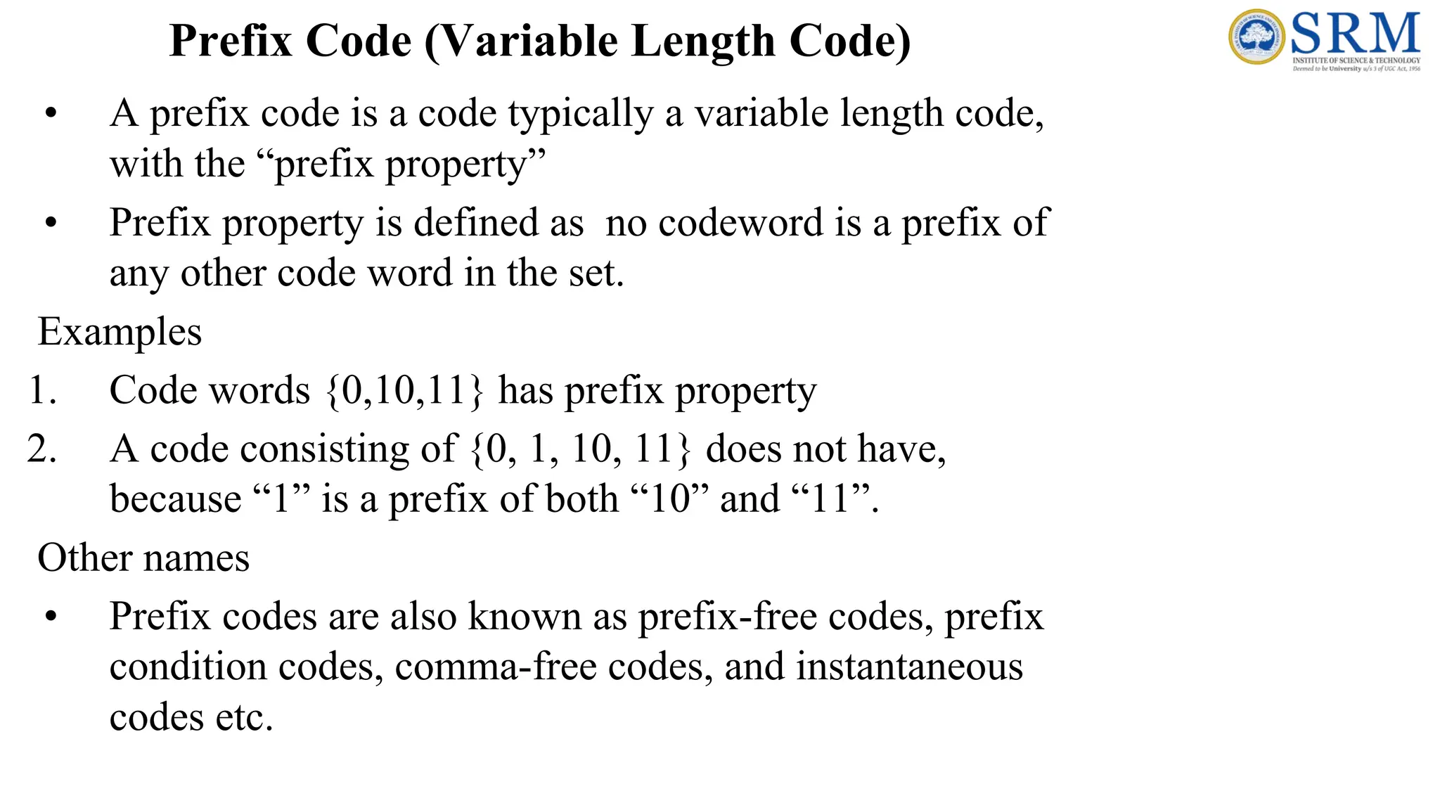
Prefix Code (VariableLength Code) • A prefix code is a code typically a variable length code, with the “prefix property” • Prefix property is defined as no codeword is a prefix of any other code word in the set. Examples 1. Code words {0,10,11} has prefix property 2. A code consisting of {0, 1, 10, 11} does not have, because “1” is a prefix of both “10” and “11”. Other names • Prefix codes are also known as prefix-free codes, prefix condition codes, comma-free codes, and instantaneous codes etc.
27.
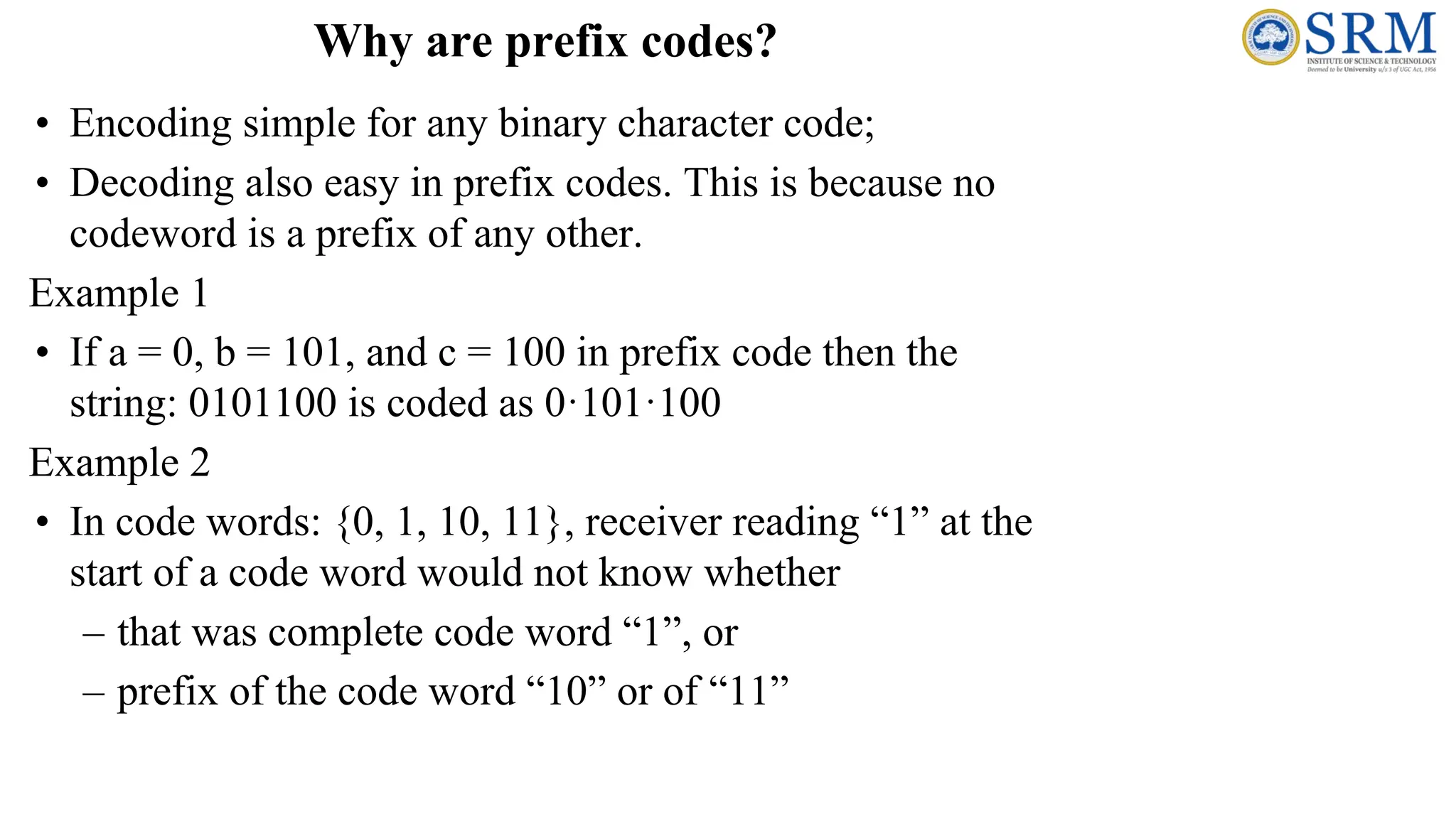
Why are prefixcodes? • Encoding simple for any binary character code; • Decoding also easy in prefix codes. This is because no codeword is a prefix of any other. Example 1 • If a = 0, b = 101, and c = 100 in prefix code then the string: 0101100 is coded as 0·101·100 Example 2 • In code words: {0, 1, 10, 11}, receiver reading “1” at the start of a code word would not know whether – that was complete code word “1”, or – prefix of the code word “10” or of “11”
28.
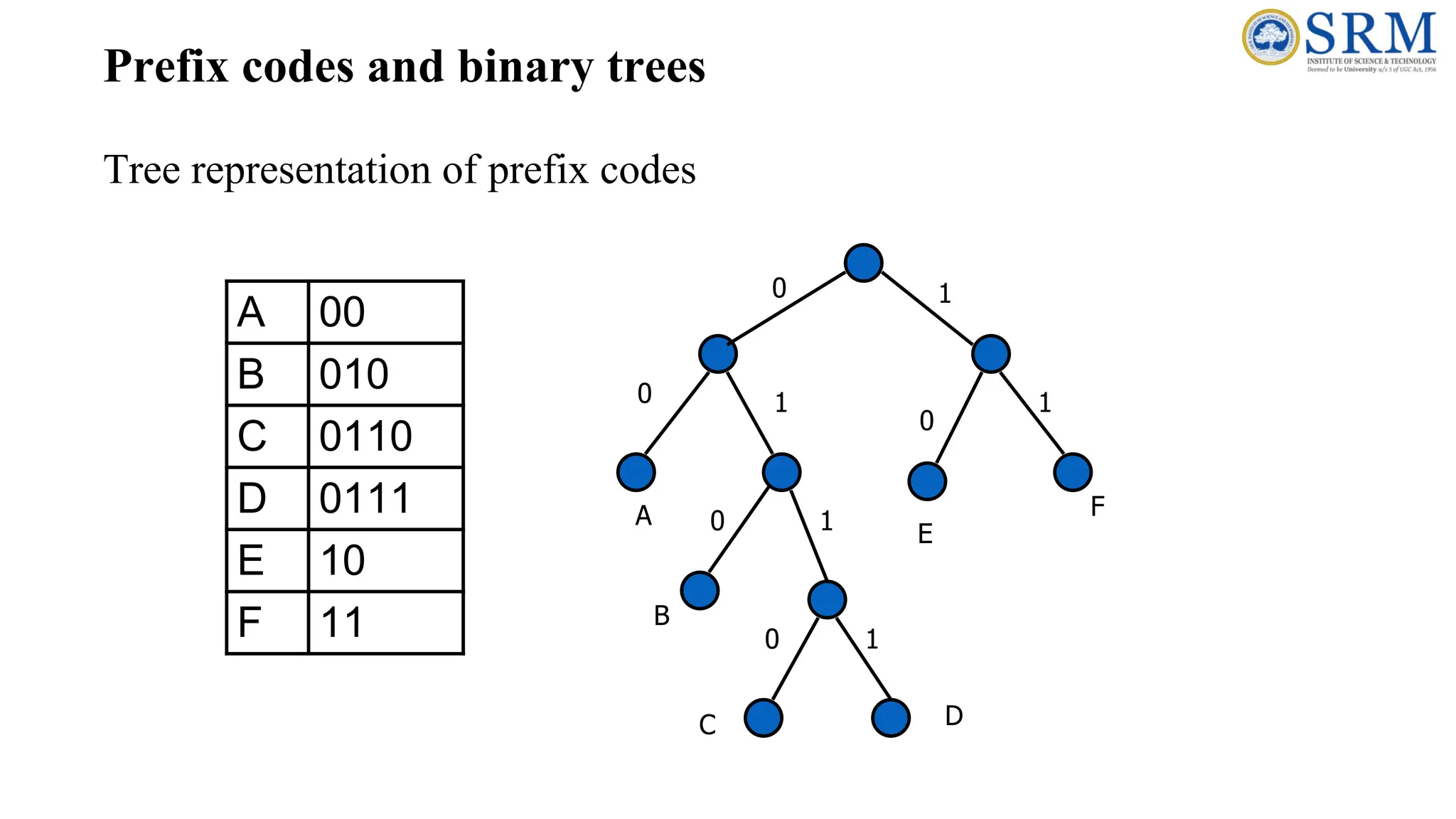
Prefix codes andbinary trees Tree representation of prefix codes A 00 B 010 C 0110 D 0111 E 10 F 11 A 0 B 0 0 0 0 1 1 1 1 1 C D E F
29.
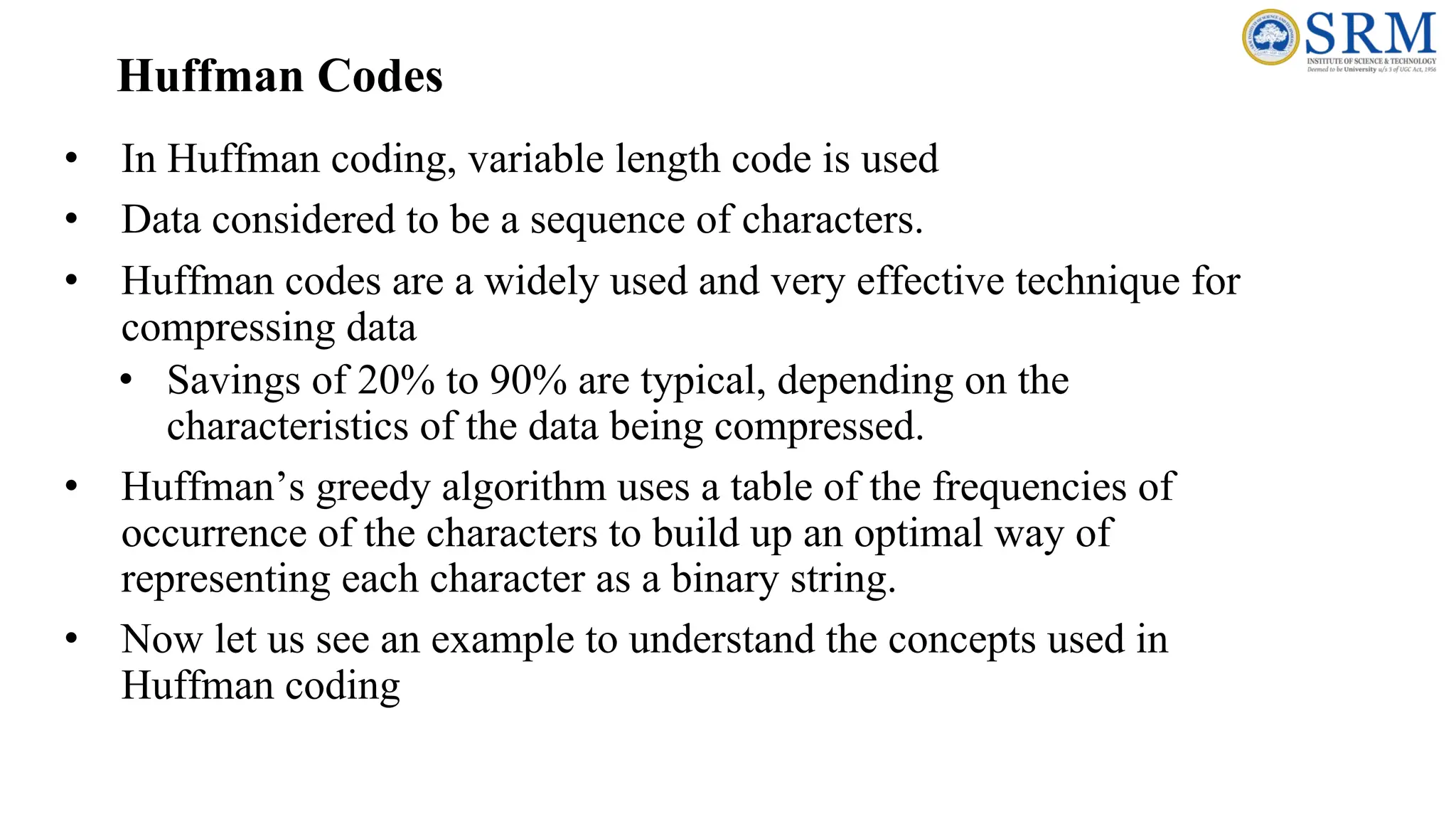
Huffman Codes • InHuffman coding, variable length code is used • Data considered to be a sequence of characters. • Huffman codes are a widely used and very effective technique for compressing data • Savings of 20% to 90% are typical, depending on the characteristics of the data being compressed. • Huffman’s greedy algorithm uses a table of the frequencies of occurrence of the characters to build up an optimal way of representing each character as a binary string. • Now let us see an example to understand the concepts used in Huffman coding
30.
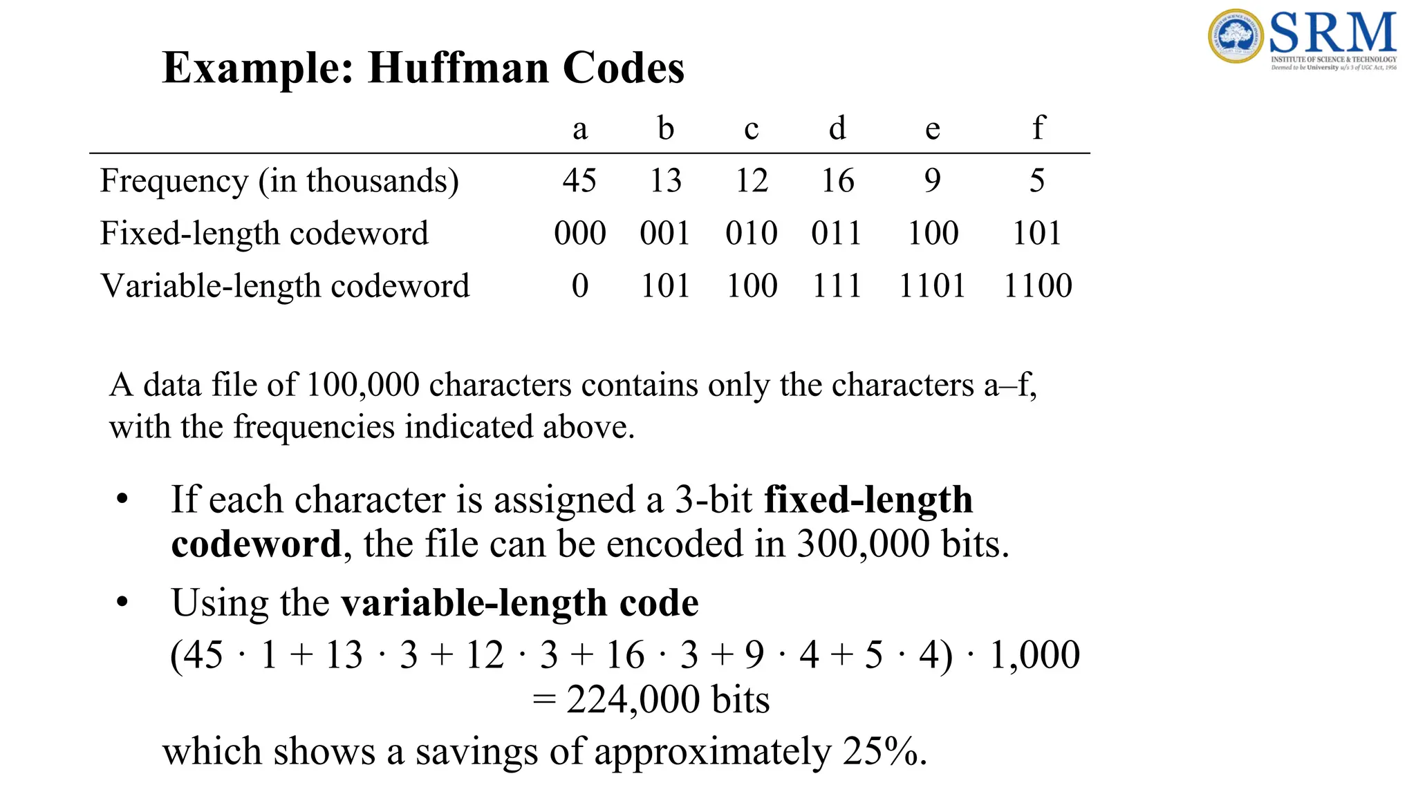
Example: Huffman Codes ab c d e f Frequency (in thousands) 45 13 12 16 9 5 Fixed-length codeword 000 001 010 011 100 101 Variable-length codeword 0 101 100 111 1101 1100 • If each character is assigned a 3-bit fixed-length codeword, the file can be encoded in 300,000 bits. • Using the variable-length code (45 · 1 + 13 · 3 + 12 · 3 + 16 · 3 + 9 · 4 + 5 · 4) · 1,000 = 224,000 bits which shows a savings of approximately 25%. A data file of 100,000 characters contains only the characters a–f, with the frequencies indicated above.
31.
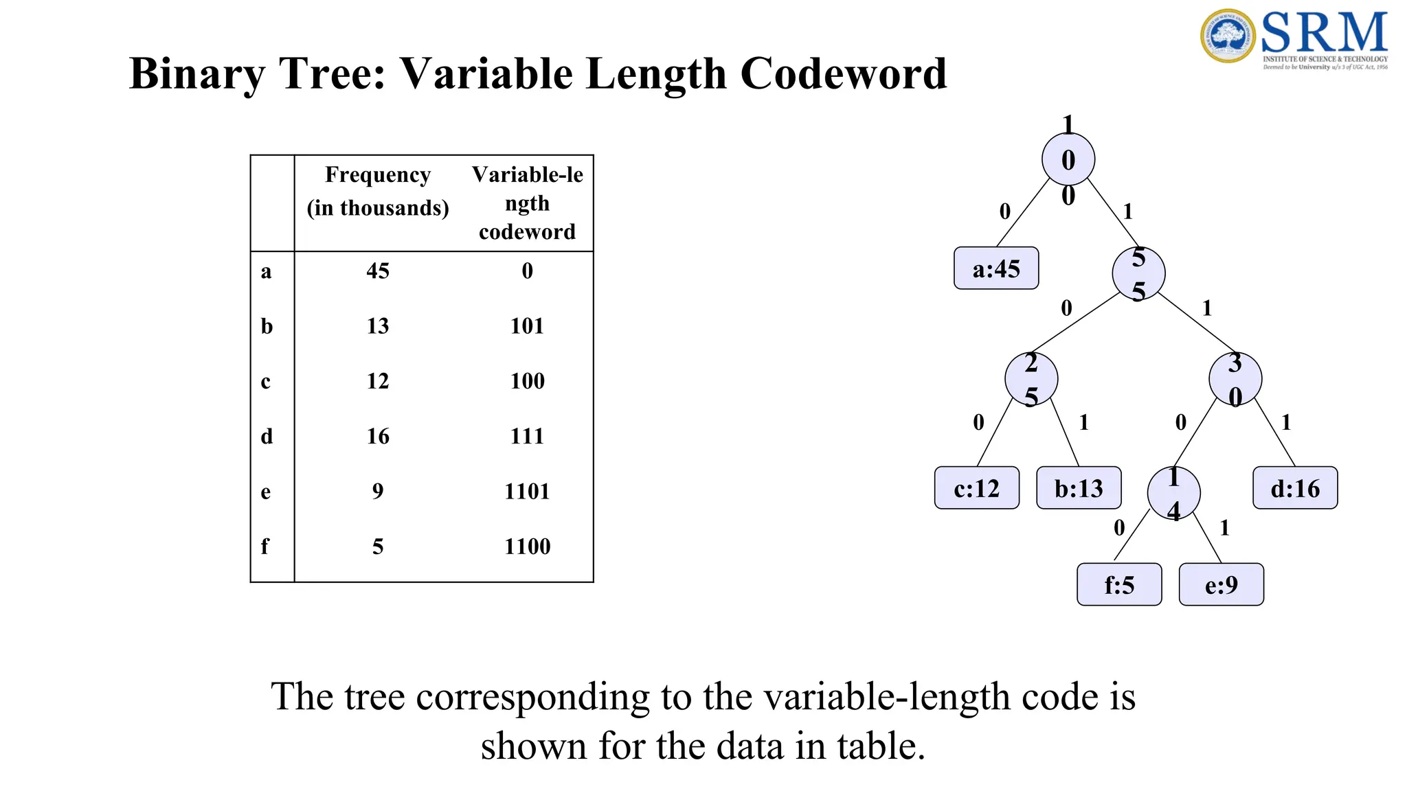
Binary Tree: VariableLength Codeword 0 1 0 0 5 5 2 5 3 0 1 4 f:5 e:9 c:12 b:13 d:16 a:45 1 0 1 0 1 0 1 0 1 Frequency (in thousands) Variable-le ngth codeword a 45 0 b 13 101 c 12 100 d 16 111 e 9 1101 f 5 1100 The tree corresponding to the variable-length code is shown for the data in table.
32.
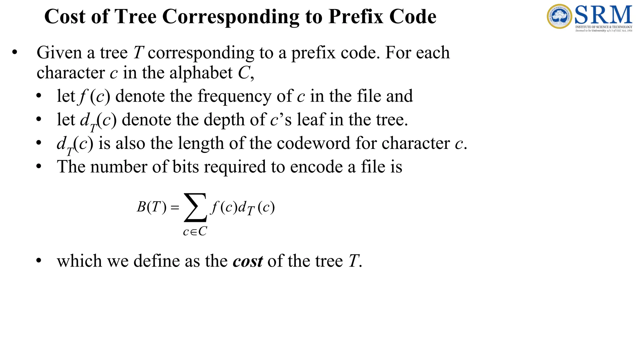
• Given atree T corresponding to a prefix code. For each character c in the alphabet C, • let f (c) denote the frequency of c in the file and • let dT (c) denote the depth of c’s leaf in the tree. • dT (c) is also the length of the codeword for character c. • The number of bits required to encode a file is • which we define as the cost of the tree T. Cost of Tree Corresponding to Prefix Code
33.
Huffman (C) 1 n← |C| 2 Q ← C 3 for i ← 1 to n - 1 4 do allocate a new node z 5 left[z] ← x ← Extract-Min (Q) 6 right[z] ← y ← Extract-Min (Q) 7 f [z] ← f [x] + f [y] 8 Insert (Q, z) 9 return Extract-Min(Q) Return root of the tree. Algorithm: Constructing a Huffman Codes
34.
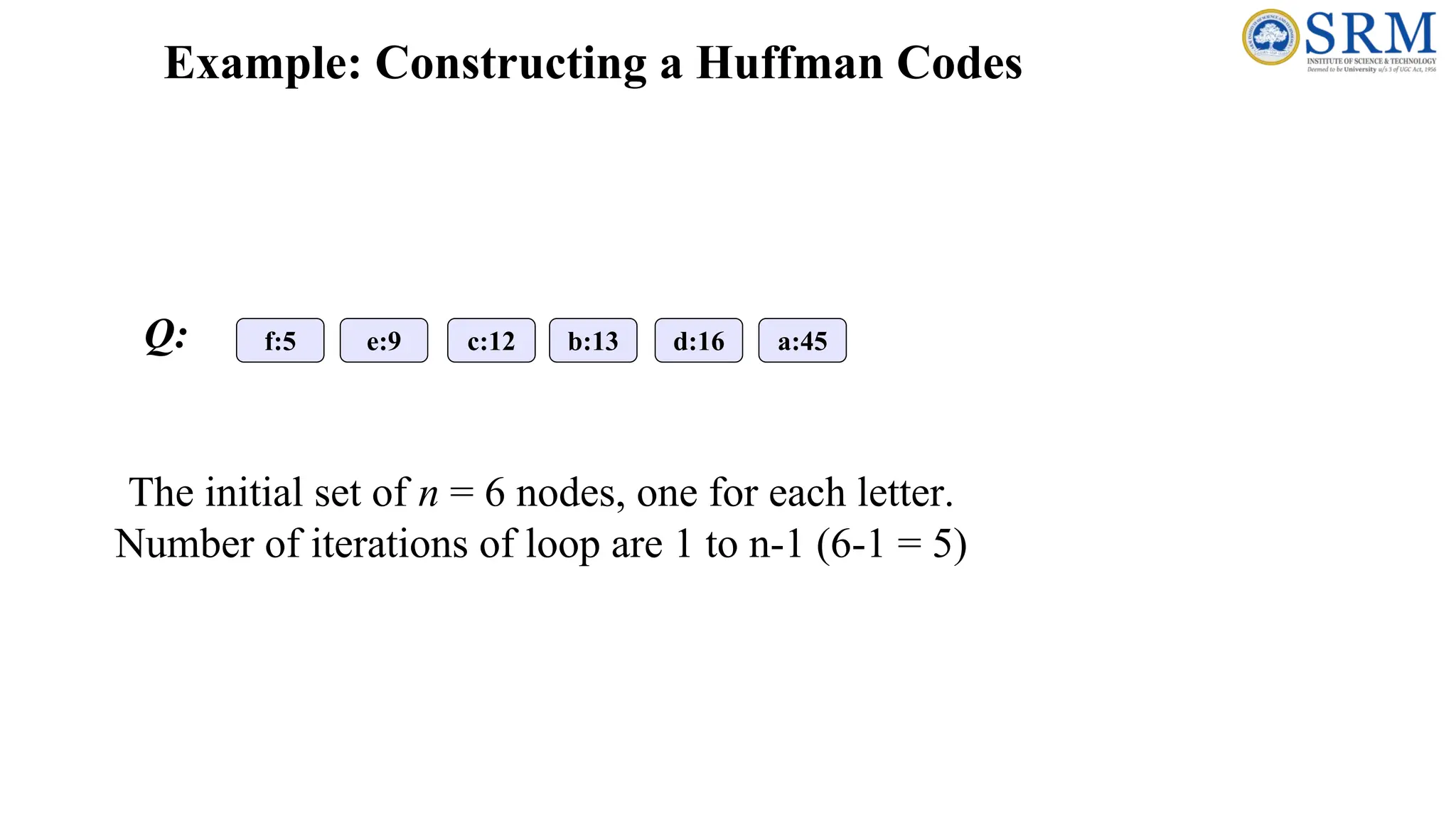
Example: Constructing aHuffman Codes a:45 b:13 c:12 d:16 e:9 f:5 The initial set of n = 6 nodes, one for each letter. Number of iterations of loop are 1 to n-1 (6-1 = 5) Q:
35.
Constructing a HuffmanCodes for i ← 1 Allocate a new node z left[z] ← x ← Extract-Min (Q) = f:5 right[z] ← y ← Extract-Min (Q) = e:9 f [z] ← f [x] + f [y] (5 + 9 = 14) Insert (Q, z) Q: d:16 a:45 b:13 c:12 0 1 4 f:5 e:9 1
36.
Constructing a HuffmanCodes for i ← 3 Allocate a new node z left[z] ← x ← Extract-Min (Q) = z:14 right[z] ← y ← Extract-Min (Q) = d:16 f [z] ← f [x] + f [y] (14 + 16 = 30) Insert (Q, z) Q: a:45 0 2 5 c:12 b:13 1 0 3 0 1 4 f:5 e:9 d:16 1 0 1 Q: a:45 d:16 0 1 4 f:5 e:9 1 0 2 5 c:12 b:13 1
37.
Constructing a HuffmanCodes for i ← 4 Allocate a new node z left[z] ← x ← Extract-Min (Q) = z:25 right[z] ← y ← Extract-Min (Q) = z:30 f [z] ← f [x] + f [y] (25 + 30 = 55) Insert (Q, z) Q: a:45 0 5 5 2 5 3 0 1 4 f:5 e:9 c:12 b:13 d:16 1 0 1 0 1 0 1 Q: a:45 0 2 5 c:12 b:13 1 0 3 0 1 4 f:5 e:9 d:16 1 0 1
38.
Constructing a HuffmanCodes for i ← 5 Allocate a new node z left[z] ← x ← Extract-Min (Q) = a:45 right[z] ← y ← Extract-Min (Q) = z:55 f [z] ← f [x] + f [y] (45 + 55 = 100) Insert (Q, z) Q: 0 1 0 0 5 5 2 5 3 0 1 4 f:5 e:9 c:12 b:13 d:16 a:45 1 0 1 0 1 0 1 0 1
39.
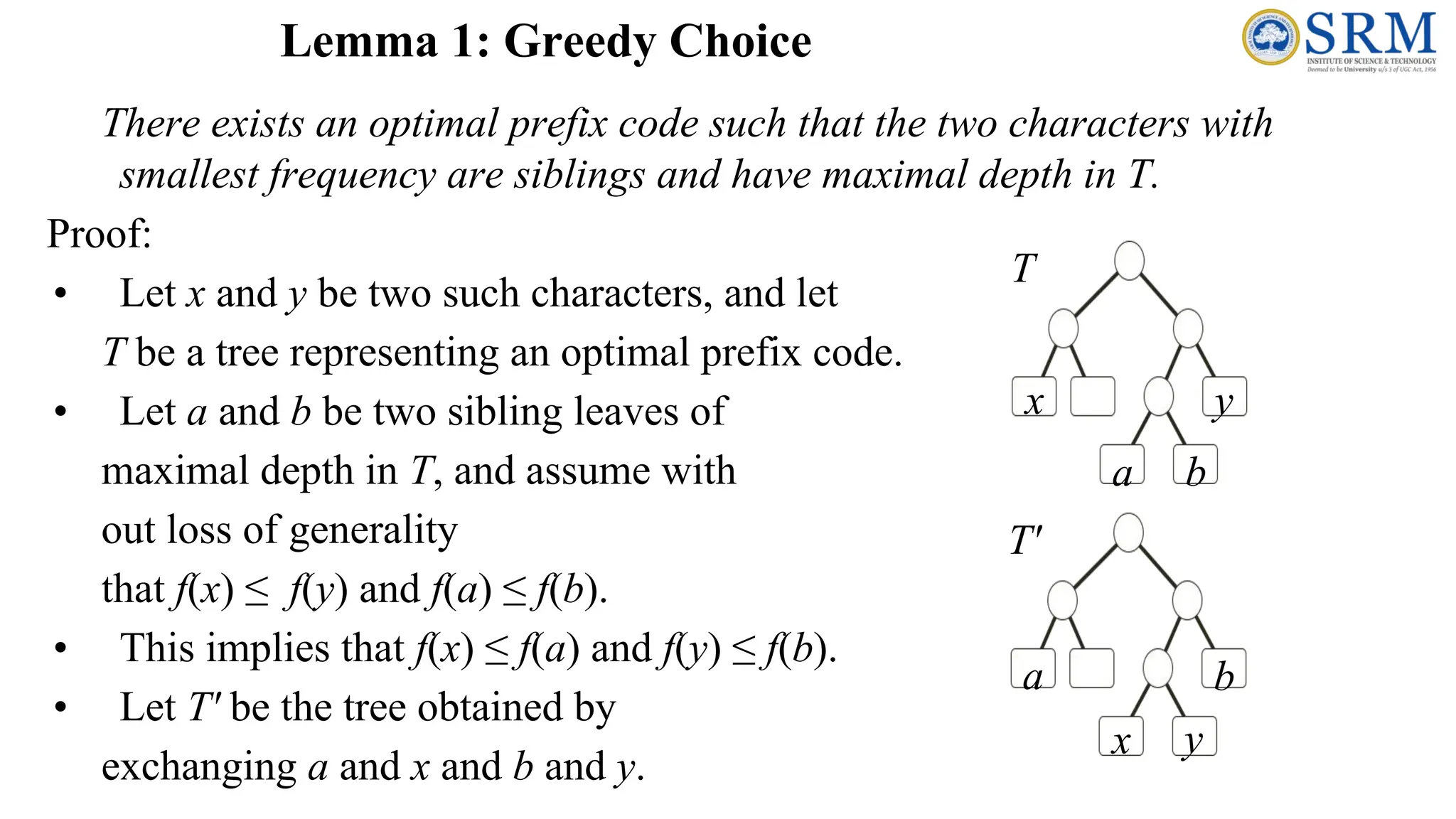
Lemma 1: GreedyChoice There exists an optimal prefix code such that the two characters with smallest frequency are siblings and have maximal depth in T. Proof: • Let x and y be two such characters, and let T be a tree representing an optimal prefix code. • Let a and b be two sibling leaves of maximal depth in T, and assume with out loss of generality that f(x) ≤ f(y) and f(a) ≤ f(b). • This implies that f(x) ≤ f(a) and f(y) ≤ f(b). • Let T' be the tree obtained by exchanging a and x and b and y. T x y b a T' x a y b
40.
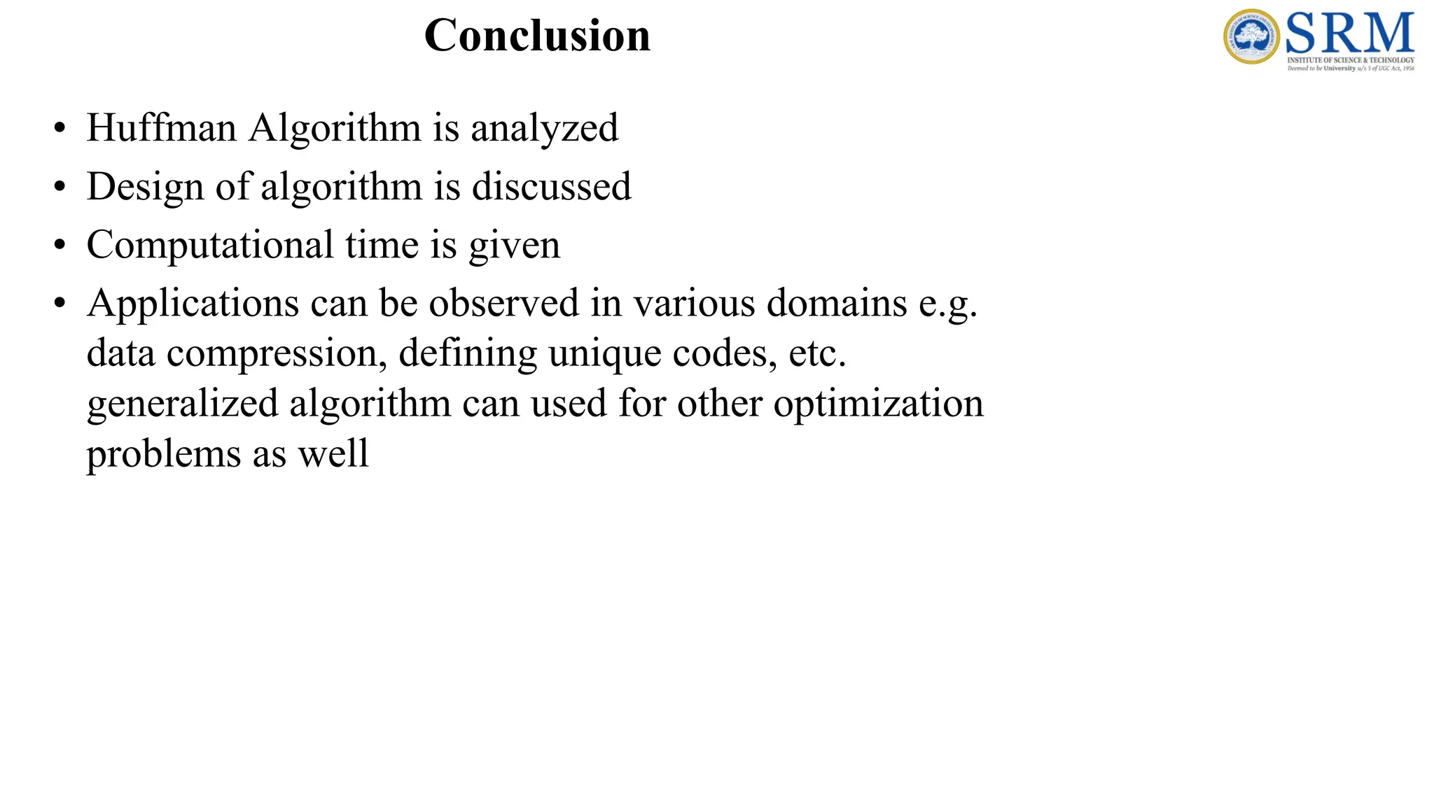
• Huffman Algorithmis analyzed • Design of algorithm is discussed • Computational time is given • Applications can be observed in various domains e.g. data compression, defining unique codes, etc. generalized algorithm can used for other optimization problems as well Conclusion
41.
Two questions •Why doesthe algorithm produce the best tree ? •How do you implement it efficiently ?
Session Learning Outcome-SLO Greedyis used in optimization problems. The algorithm makes the optimal choice at each step as it attempts to find the overall optimal way to solve the entire problem 43
44.
44 GREEDY INTRODUCTION Greedy algorithmsare simple and straightforward. They are shortsighted in their approach A greedy algorithm is similar to a dynamic programming algorithm, but the difference is that solutions to the sub problems do not have to be known at each stage, instead a "greedy" choice can be made of what looks best for the moment.
45.
45 GREEDY INTRODUCTION • Manyreal-world problems are optimization problems in that they attempt to find an optimal solution among many possible candidate solutions. • An optimization problem is one in which you want to find, not just a solution, but the best solution • A “greedy algorithm” sometimes works well for optimization problems • A greedy algorithm works in phases. At each phase: You take the best you can get right now, without regard for future consequences. It hope that by choosing a local optimum at each step, you will end up at a global optimum.
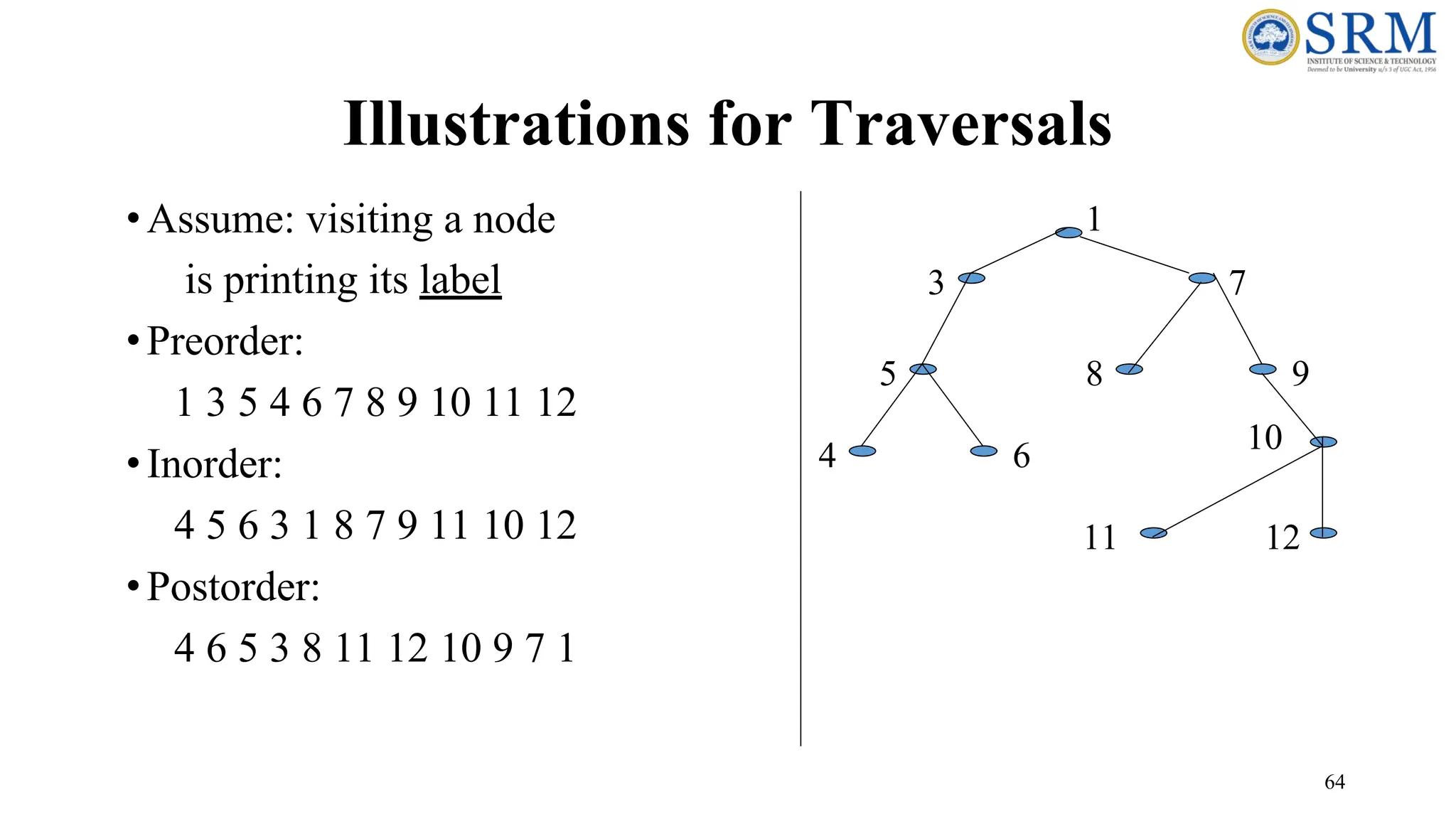
61 Tree Traversal •Traversal isthe process of visiting every node once •Visiting a node entails doing some processing at that node, but when describing a traversal strategy, we need not concern ourselves with what that processing is
62.
62 Binary Tree TraversalTechniques •Three recursive techniques for binary tree traversal •In each technique, the left subtree is traversed recursively, the right subtree is traversed recursively, and the root is visited •What distinguishes the techniques from one another is the order of those 3 tasks
63.
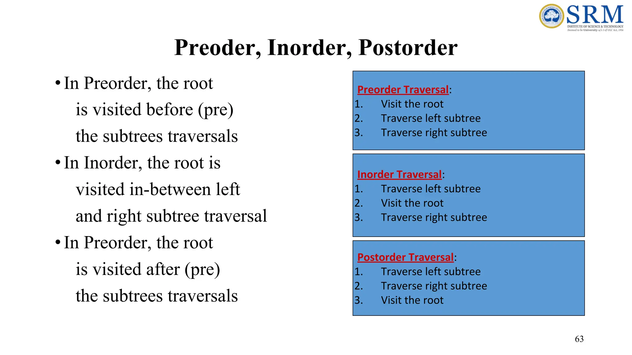
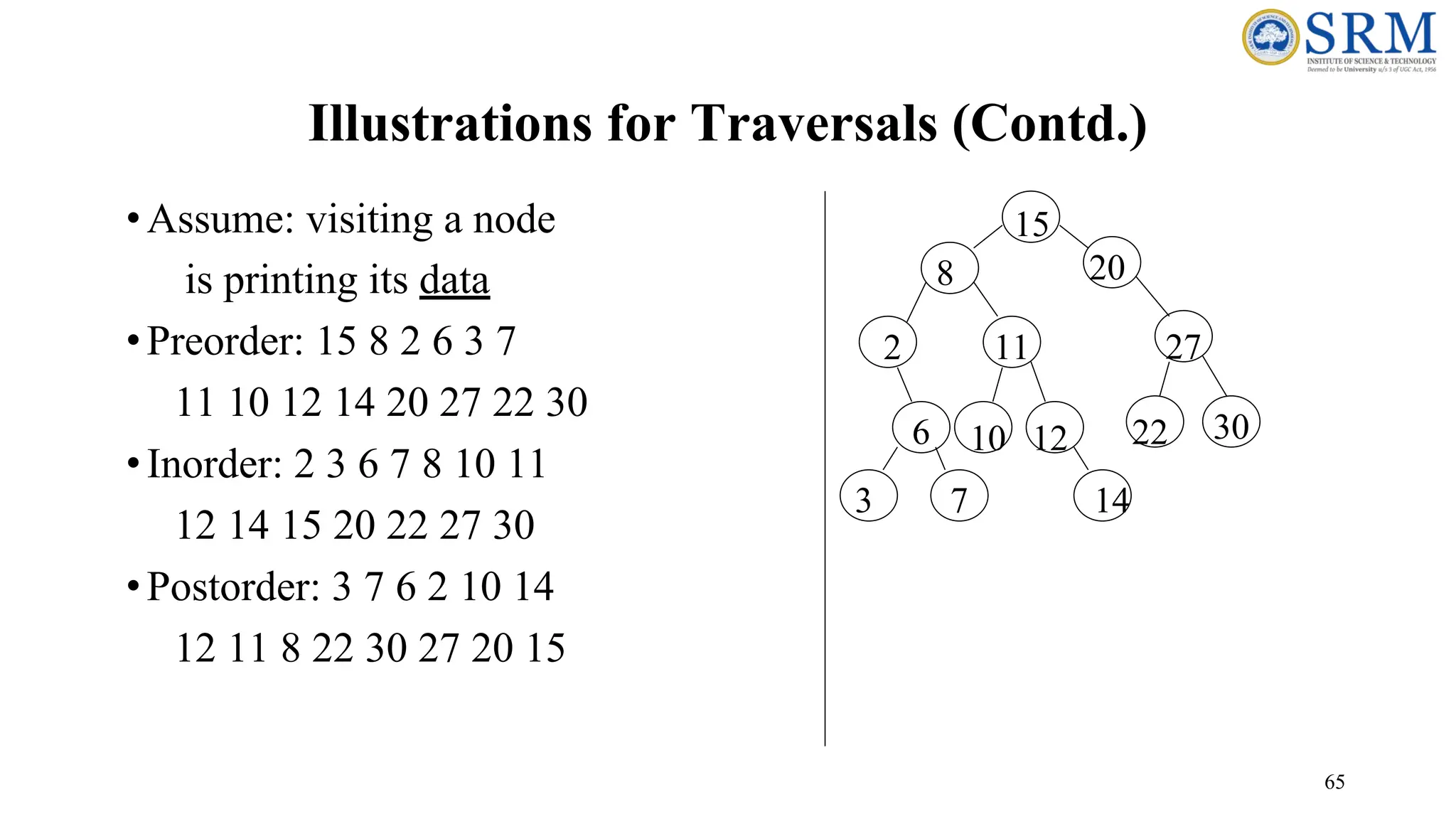
63 Preoder, Inorder, Postorder •InPreorder, the root is visited before (pre) the subtrees traversals •In Inorder, the root is visited in-between left and right subtree traversal •In Preorder, the root is visited after (pre) the subtrees traversals Preorder Traversal: 1. Visit the root 2. Traverse left subtree 3. Traverse right subtree Inorder Traversal: 1. Traverse left subtree 2. Visit the root 3. Traverse right subtree Postorder Traversal: 1. Traverse left subtree 2. Traverse right subtree 3. Visit the root
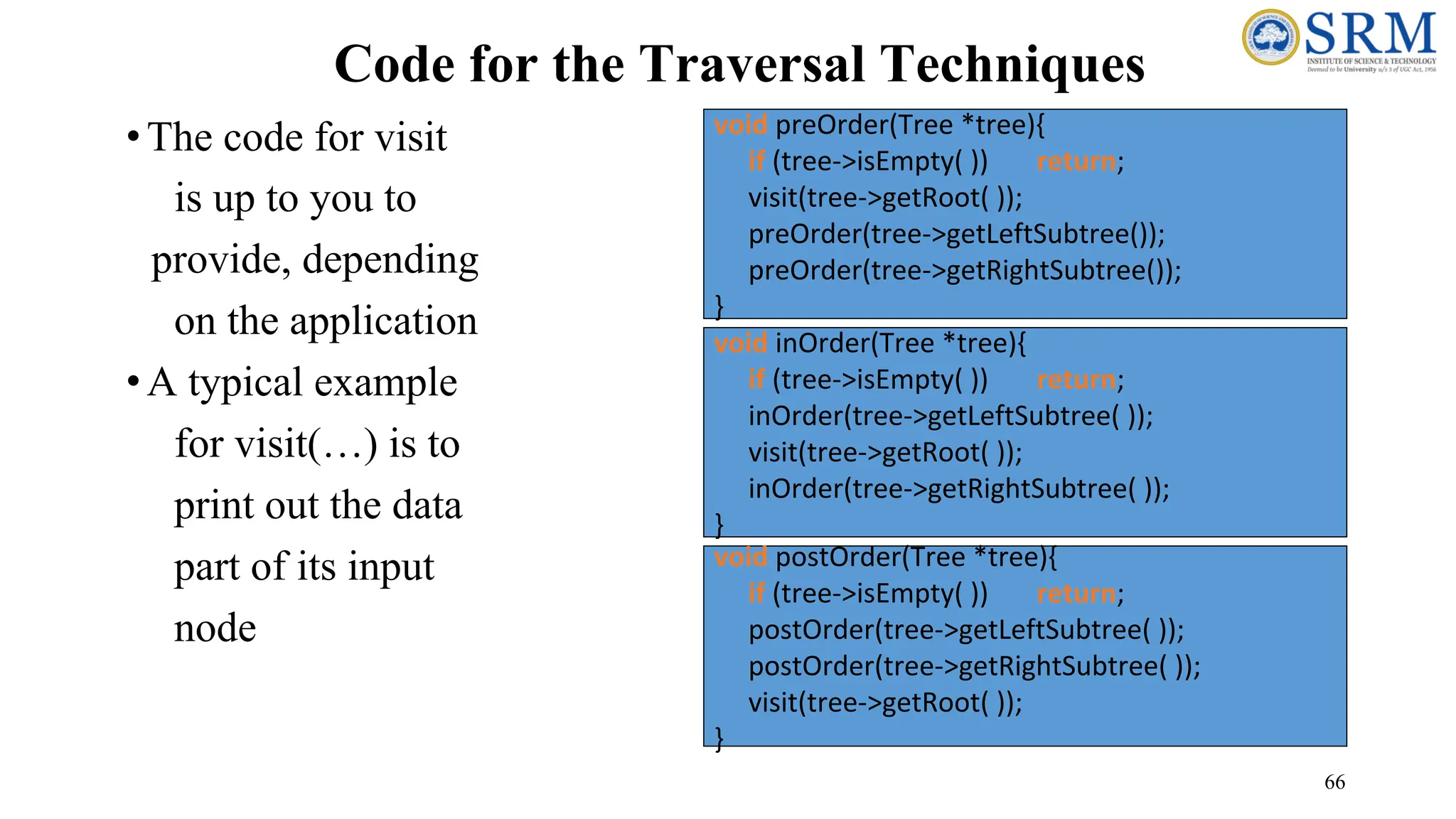
66 Code for theTraversal Techniques •The code for visit is up to you to provide, depending on the application •A typical example for visit(…) is to print out the data part of its input node void inOrder(Tree *tree){ if (tree->isEmpty( )) return; inOrder(tree->getLeftSubtree( )); visit(tree->getRoot( )); inOrder(tree->getRightSubtree( )); } void preOrder(Tree *tree){ if (tree->isEmpty( )) return; visit(tree->getRoot( )); preOrder(tree->getLeftSubtree()); preOrder(tree->getRightSubtree()); } void postOrder(Tree *tree){ if (tree->isEmpty( )) return; postOrder(tree->getLeftSubtree( )); postOrder(tree->getRightSubtree( )); visit(tree->getRoot( )); }
Session Outcomes •Apply andanalyse different problems using greedy techniques •Evaluate the real time problems •Analyse the different trees and find the low cost spanning tree
71.
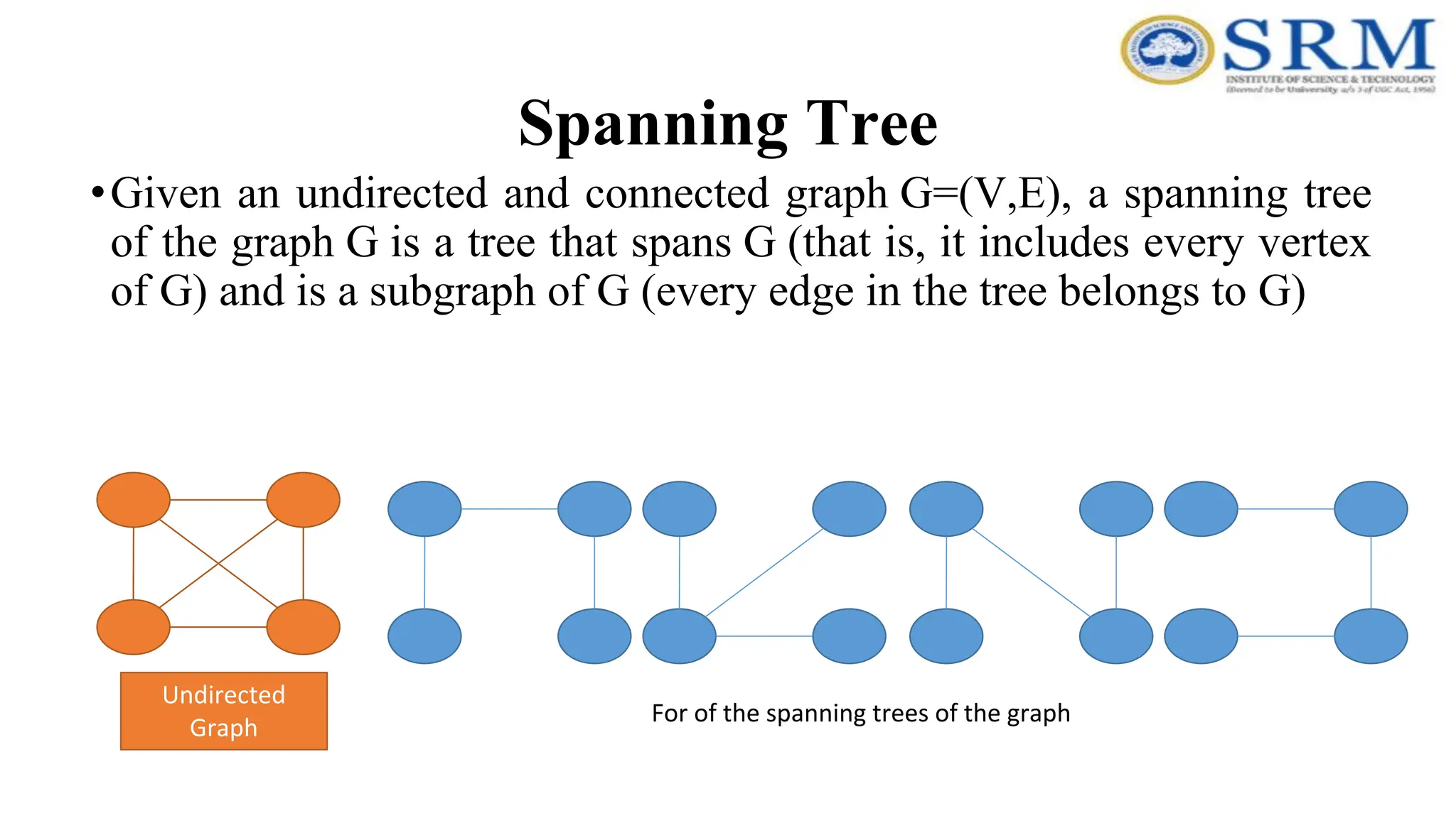
Spanning Tree •Given anundirected and connected graph G=(V,E), a spanning tree of the graph G is a tree that spans G (that is, it includes every vertex of G) and is a subgraph of G (every edge in the tree belongs to G) Undirected Graph For of the spanning trees of the graph
72.
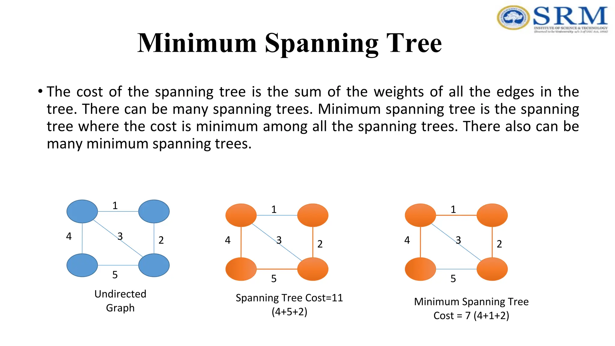
Minimum Spanning Tree •The cost of the spanning tree is the sum of the weights of all the edges in the tree. There can be many spanning trees. Minimum spanning tree is the spanning tree where the cost is minimum among all the spanning trees. There also can be many minimum spanning trees. 4 1 5 3 2 4 1 5 3 2 4 1 5 3 2 Undirected Graph Spanning Tree Cost=11 (4+5+2) Minimum Spanning Tree Cost = 7 (4+1+2)
73.
Applications – MST •Minimumspanning tree has direct application in the design of networks. It is used in algorithms approximating the travelling salesman problem, multi-terminal minimum cut problem and minimum-cost weighted perfect matching. Other practical applications are: •Cluster Analysis •Handwriting recognition •Image segmentation
74.
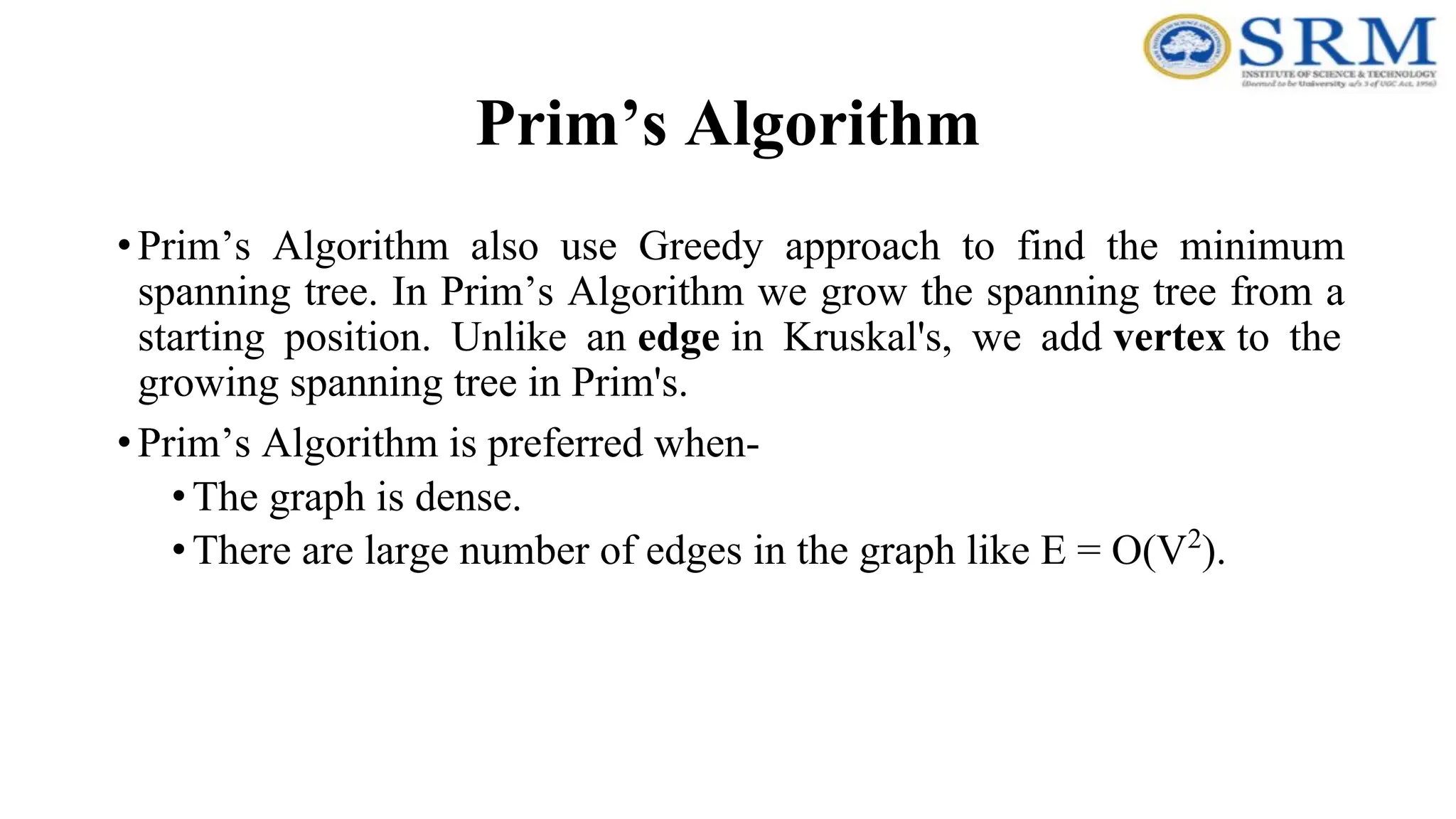
Prim’s Algorithm •Prim’s Algorithmalso use Greedy approach to find the minimum spanning tree. In Prim’s Algorithm we grow the spanning tree from a starting position. Unlike an edge in Kruskal's, we add vertex to the growing spanning tree in Prim's. •Prim’s Algorithm is preferred when- •The graph is dense. •There are large number of edges in the graph like E = O(V2 ).
75.
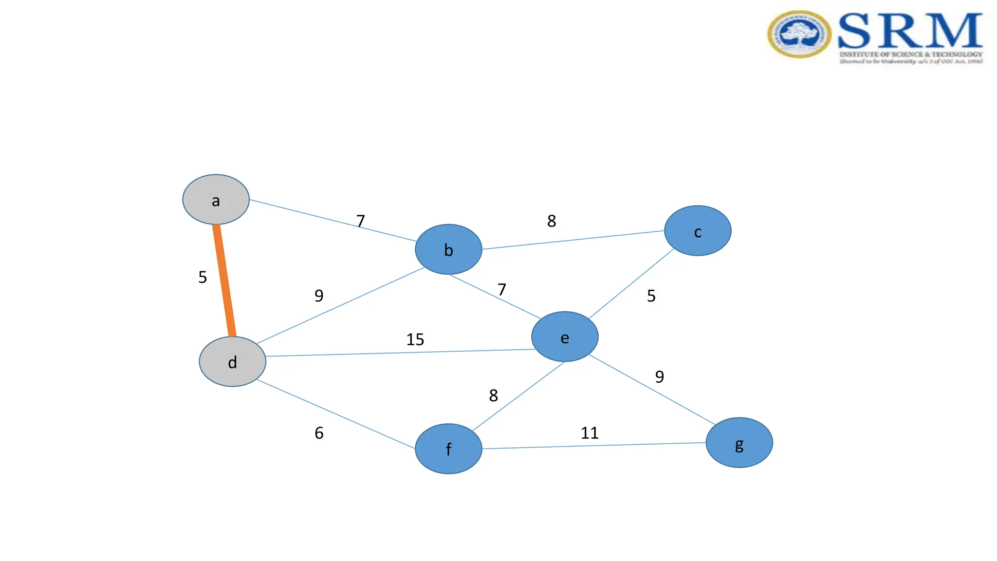
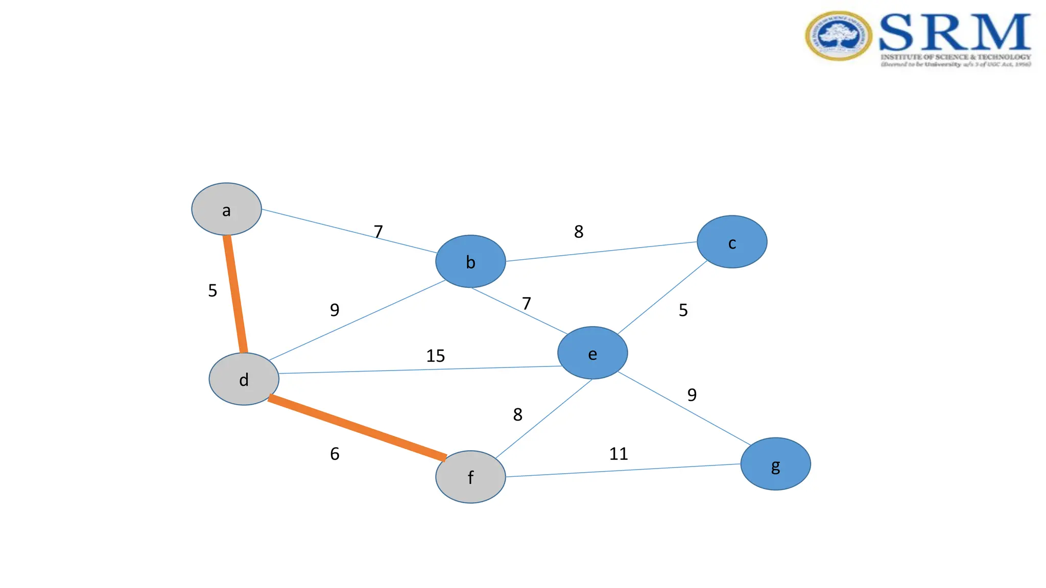
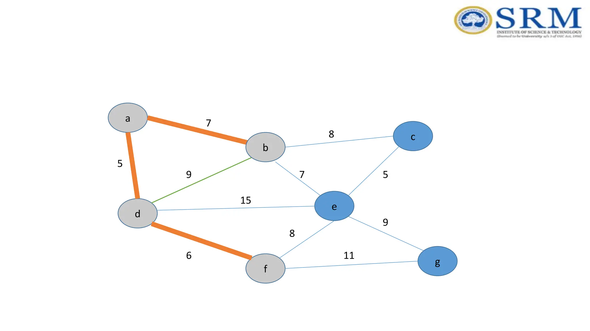
Steps for findingMST - Prim’s Algorithm Step 1: Select any vertex Step 2: Select the shortest edge connected to that vertex Step 3: Select the shortest edge connected to any vertex already connected Step 4: Repeat step 3 until all vertices have been connected
76.
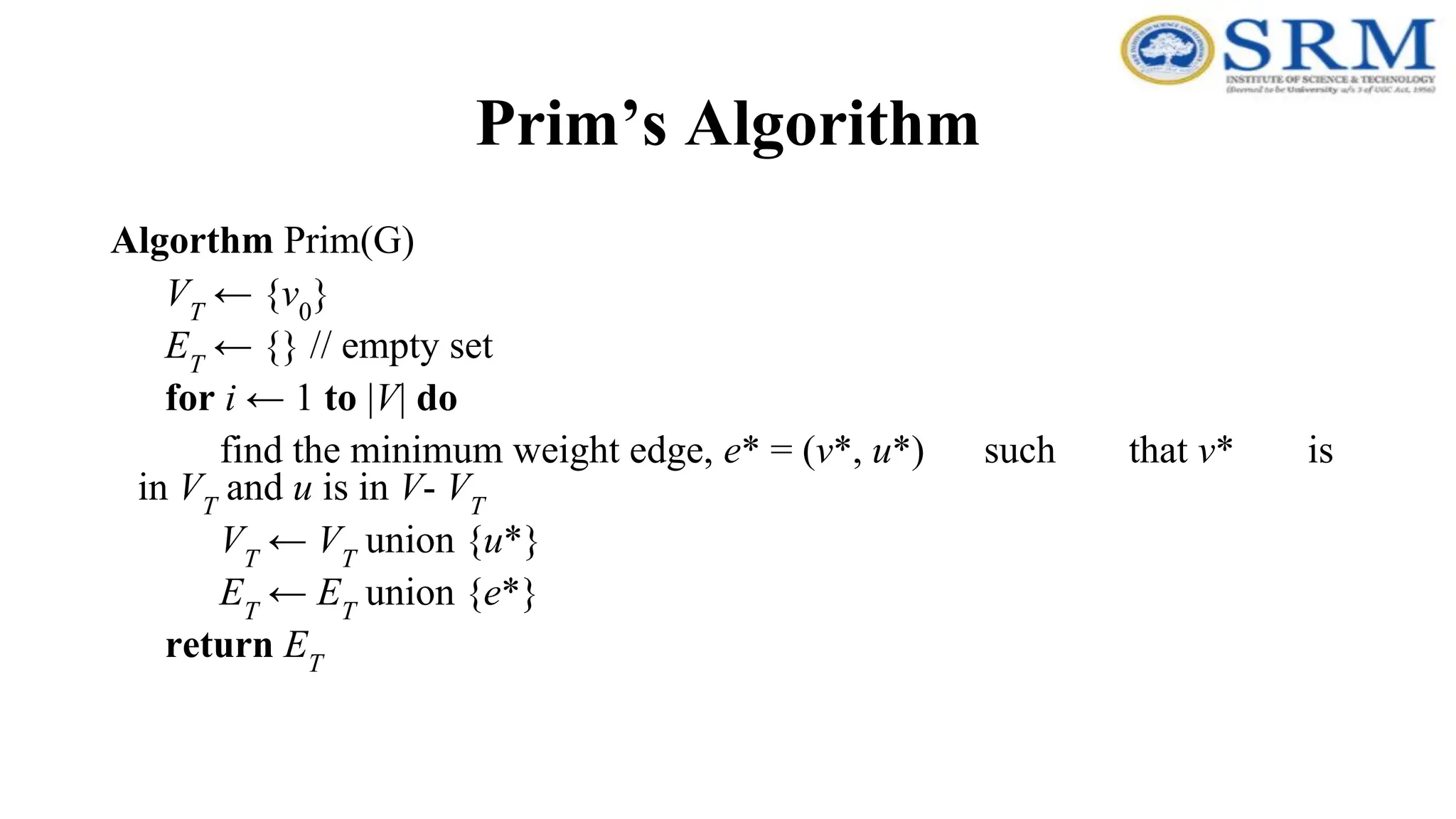
Prim’s Algorithm Algorthm Prim(G) VT ←{v0 } ET ← {} // empty set for i ← 1 to |V| do find the minimum weight edge, e* = (v*, u*) such that v* is in VT and u is in V- VT VT ← VT union {u*} ET ← ET union {e*} return ET
77.
Time Complexity –Prim’sAlgorithm • If adjacency list is used to represent the graph, then using breadth first search, all the vertices can be traversed in O(V + E) time. • We traverse all the vertices of graph using breadth first search and use a min heap for storing the vertices not yet included in the MST. • To get the minimum weight edge, we use min heap as a priority queue. • Min heap operations like extracting minimum element and decreasing key value takes O(logV) time. • So, overall time complexity • = O(E + V) x O(logV) • = O((E + V)logV) • = O(ElogV) This time complexity can be improved and reduced to O(E + VlogV) using Fibonacci heap.
78.
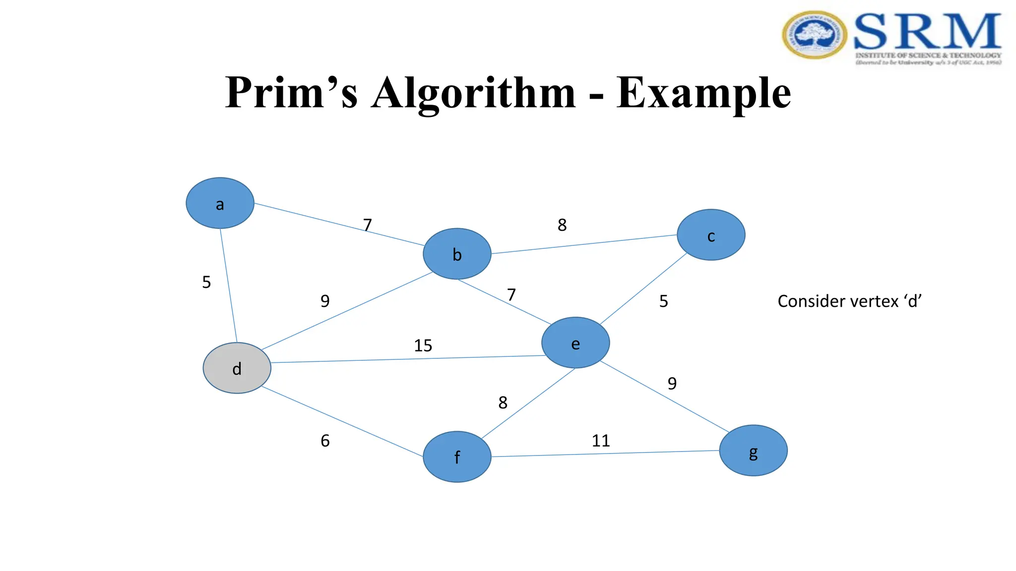
Prim’s Algorithm -Example a g c b e f d 5 7 9 7 5 8 8 15 6 9 11 Consider vertex ‘d’
Real-time Application –Prim’s Algorithm •Network for roads and Rail tracks connecting all the cities. •Irrigation channels and placing microwave towers •Designing a fiber-optic grid or ICs. •Travelling Salesman Problem. •Cluster analysis. •Path finding algorithms used in AI. •Game Development •Cognitive Science
86.
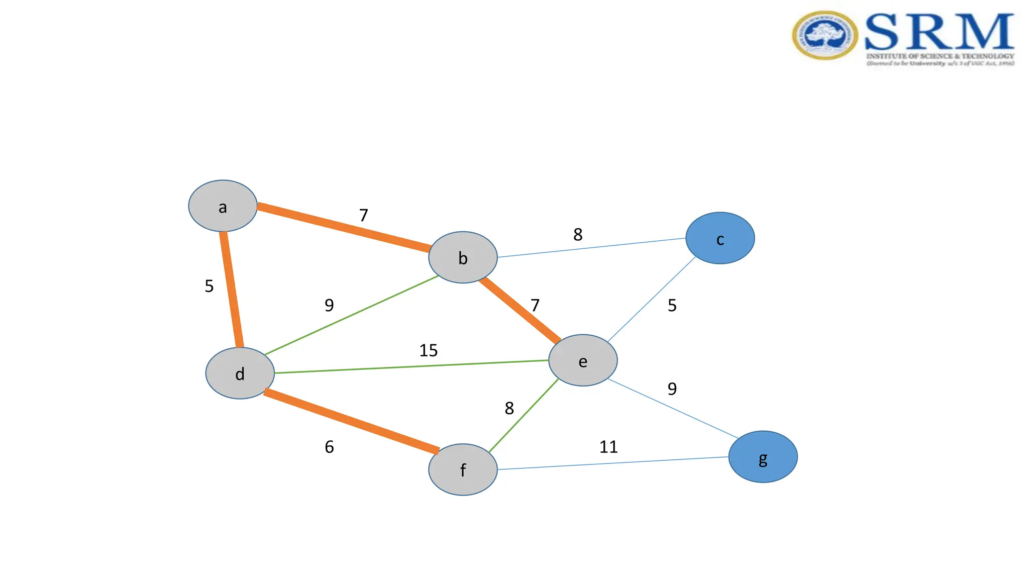
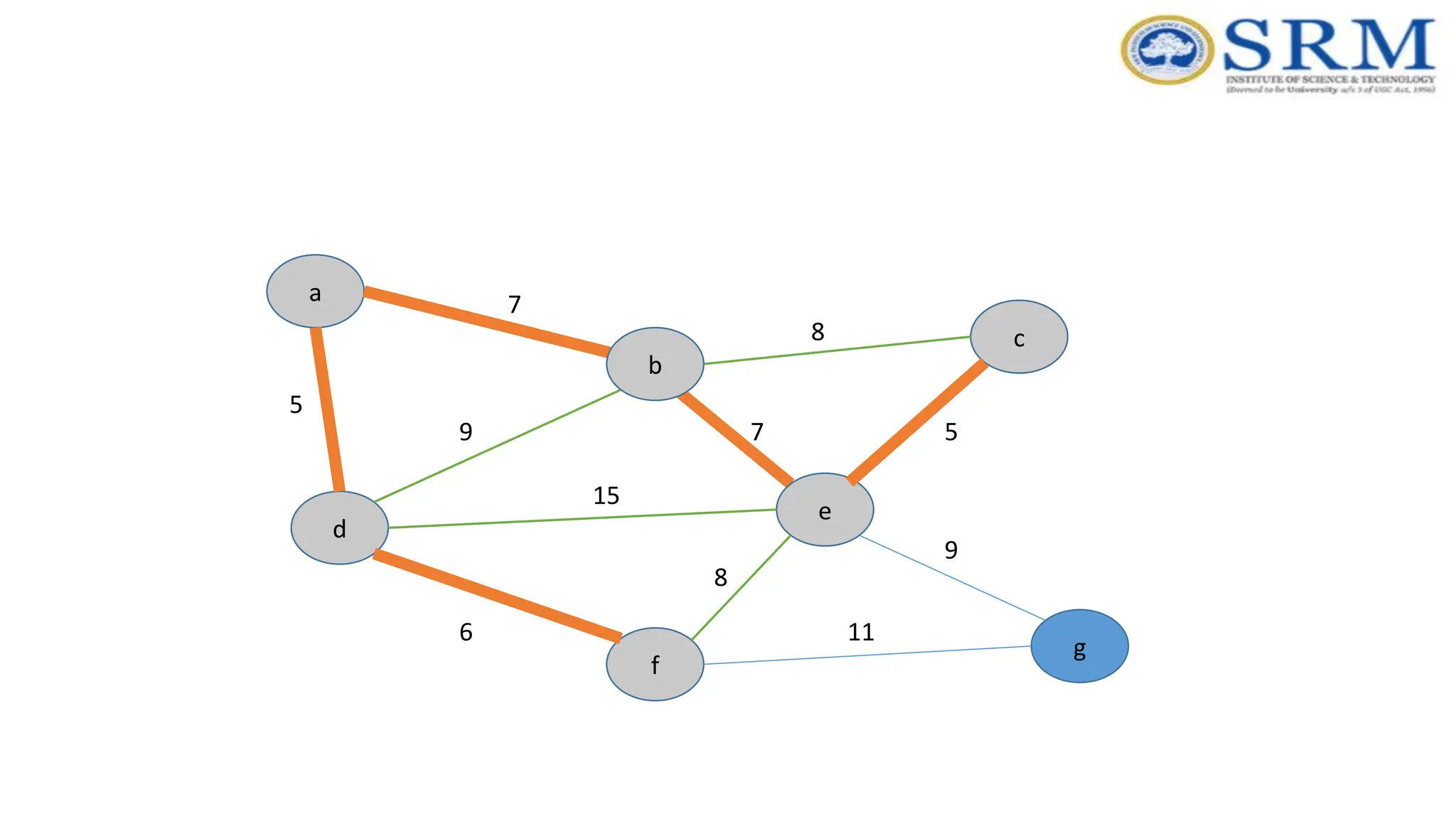
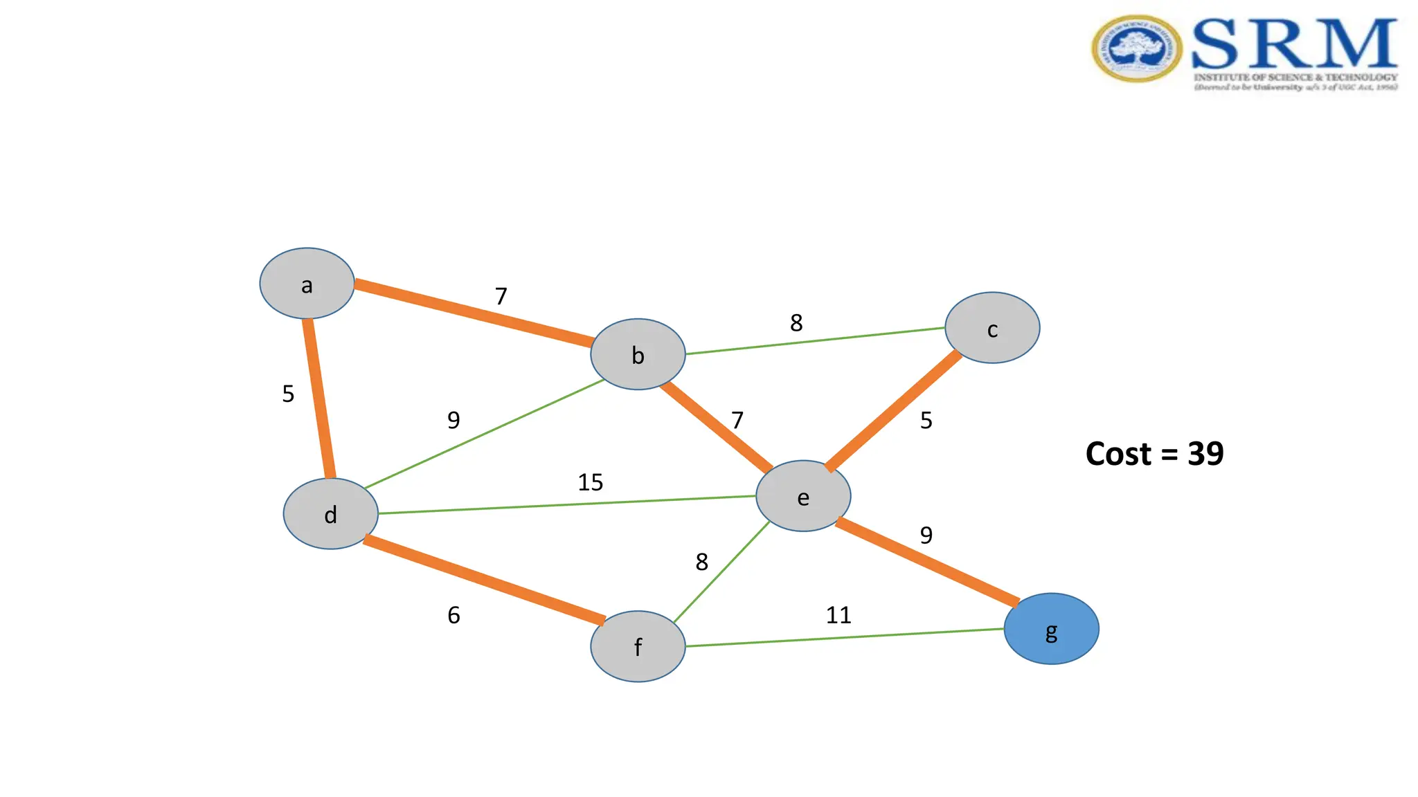
Minimum Spanning tree– Kruskal’s Algorithm •Kruskal’s Algorithm builds the spanning tree by adding edges one by one into a growing spanning tree. •Kruskal's algorithm follows greedy approach as in each iteration it finds an edge which has least weight and add it to the growing spanning tree. •Kruskal’s Algorithm is preferred when- •The graph is sparse. •There are less number of edges in the graph like E = O(V) •The edges are already sorted or can be sorted in linear time.
87.
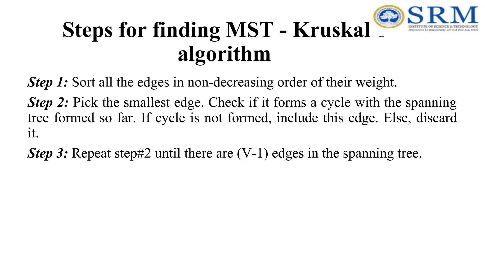
Steps for findingMST - Kruskal’s algorithm Step 1: Sort all the edges in non-decreasing order of their weight. Step 2: Pick the smallest edge. Check if it forms a cycle with the spanning tree formed so far. If cycle is not formed, include this edge. Else, discard it. Step 3: Repeat step#2 until there are (V-1) edges in the spanning tree.
88.
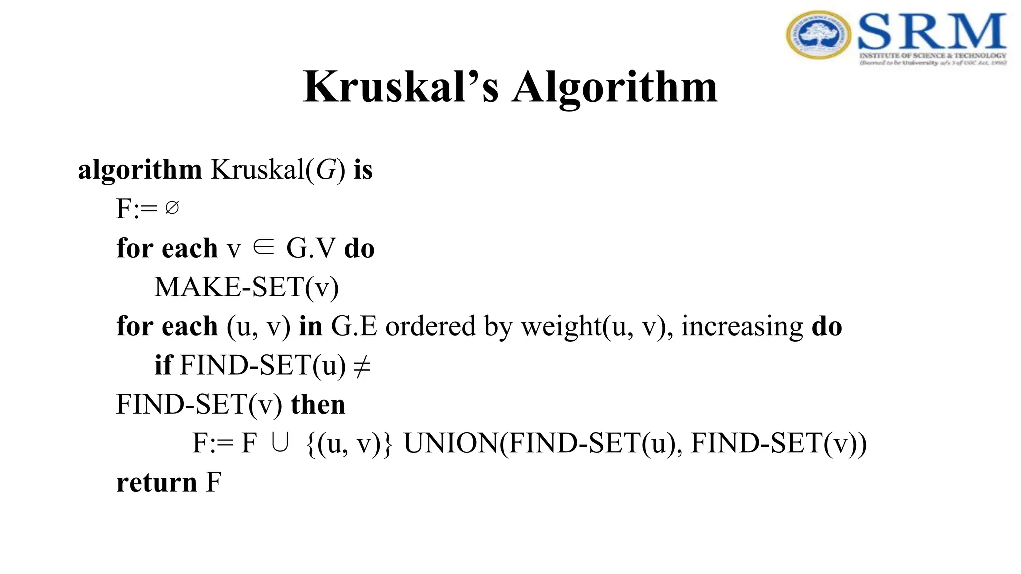
Kruskal’s Algorithm algorithm Kruskal(G)is F:= ∅ for each v ∈ G.V do MAKE-SET(v) for each (u, v) in G.E ordered by weight(u, v), increasing do if FIND-SET(u) ≠ FIND-SET(v) then F:= F ∪ {(u, v)} UNION(FIND-SET(u), FIND-SET(v)) return F
89.
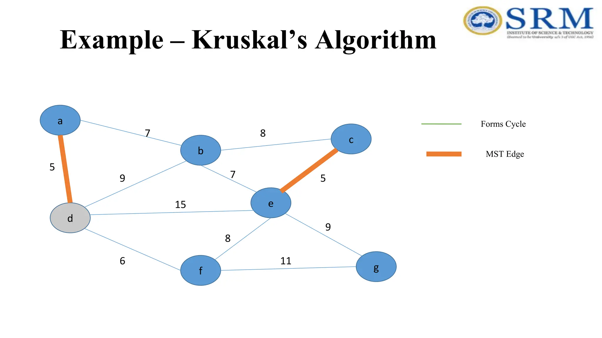
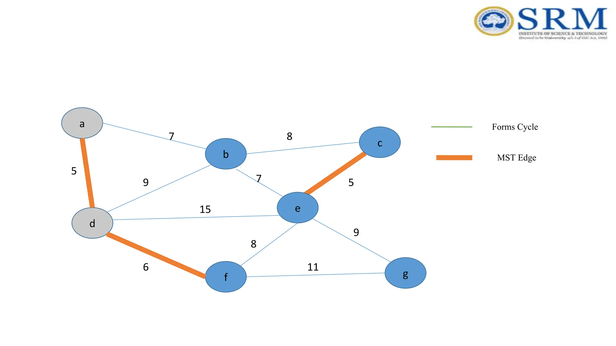
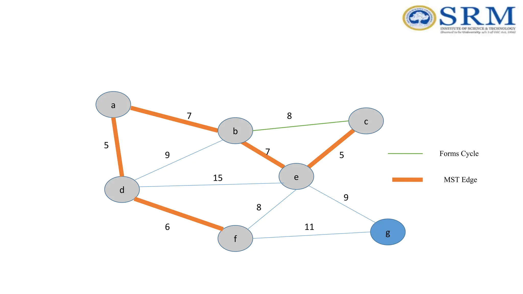
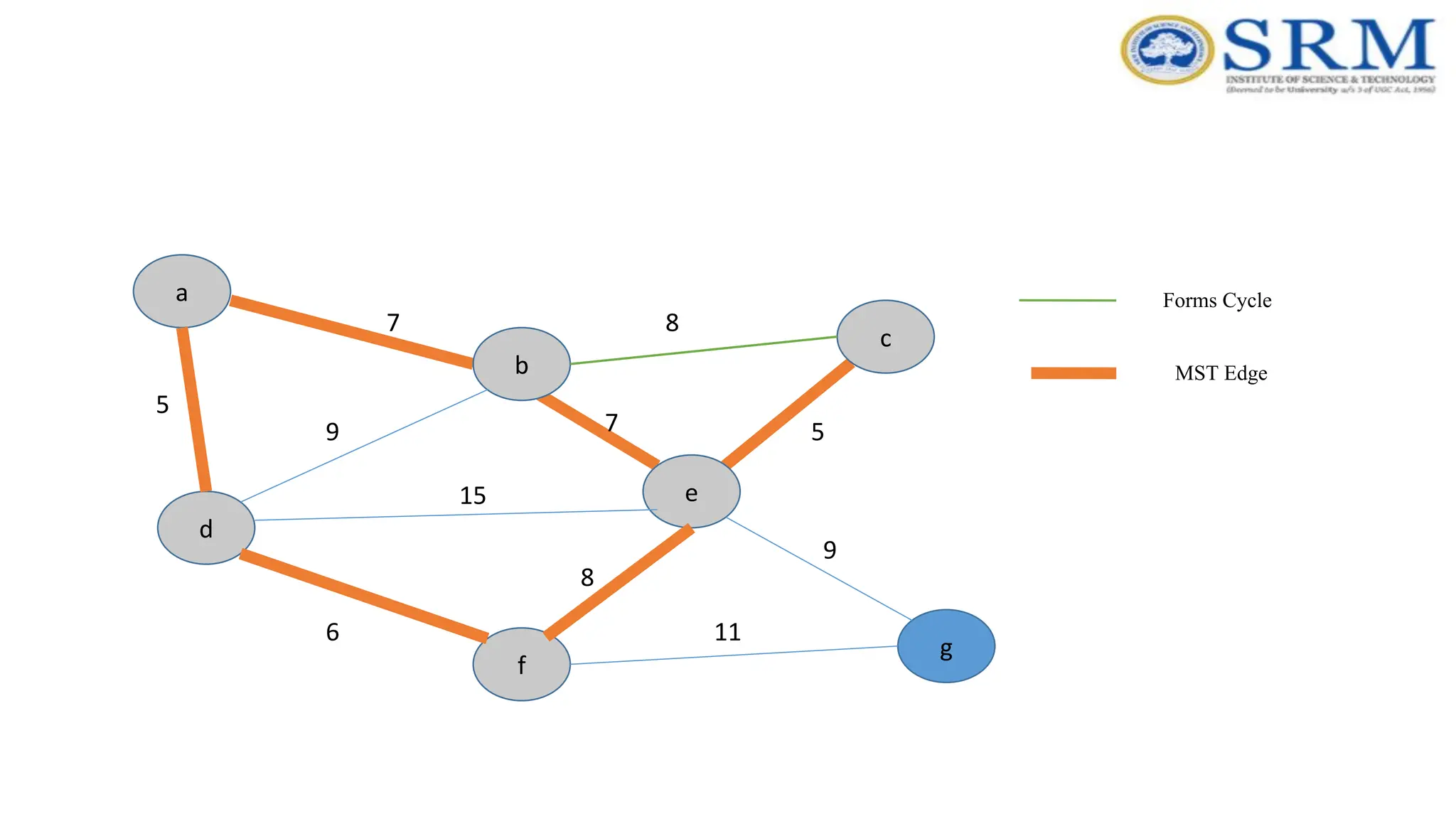
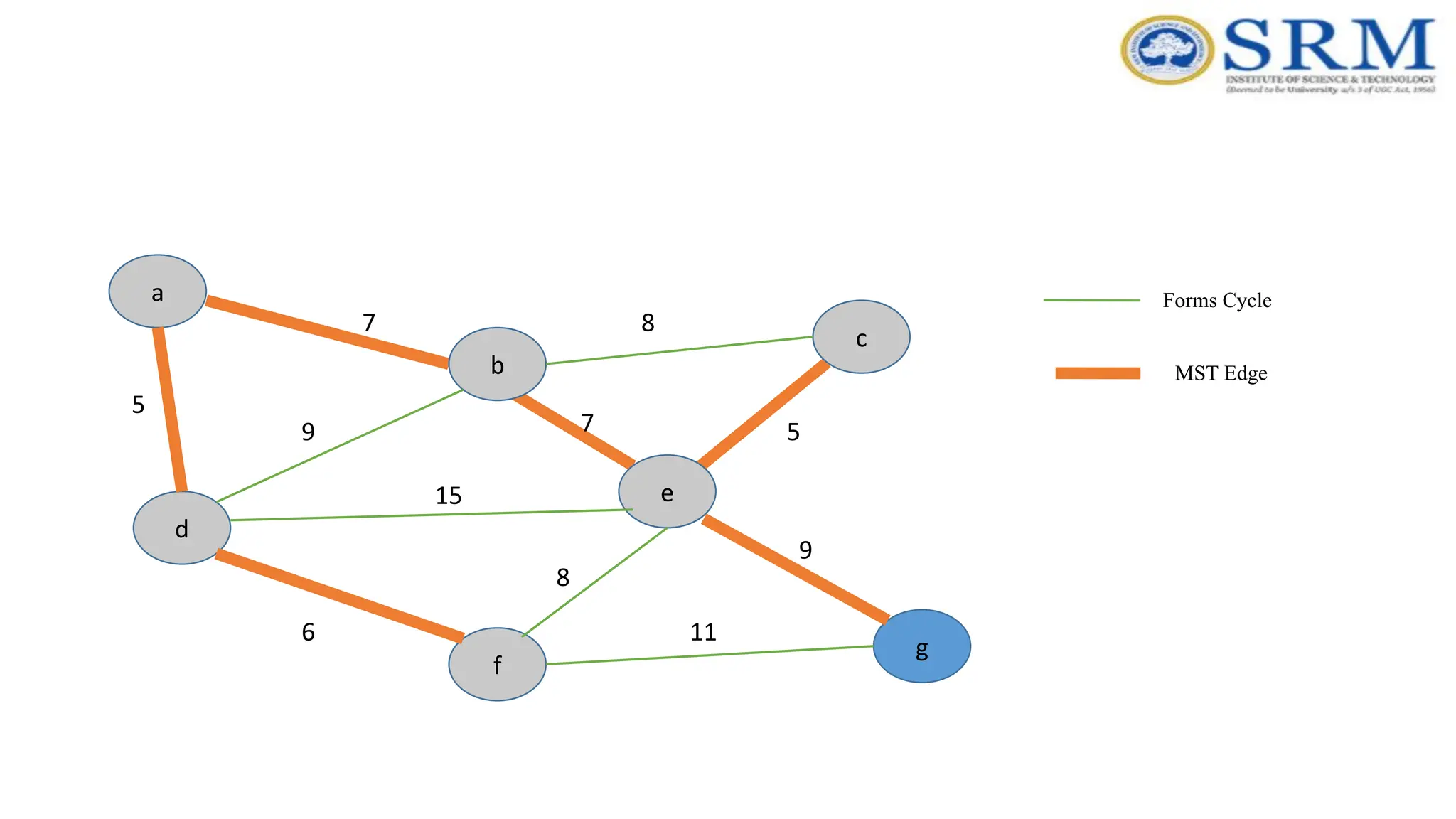
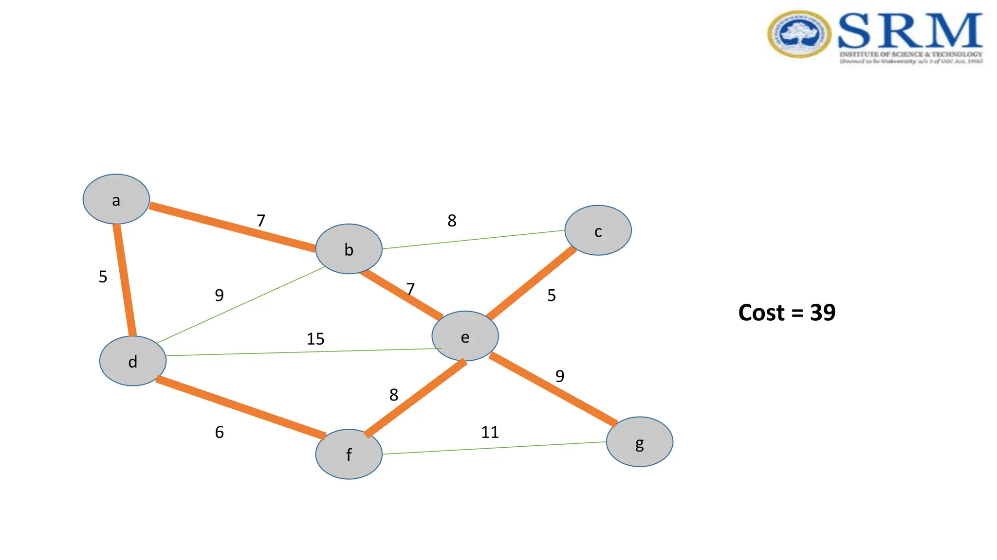
Example – Kruskal’sAlgorithm a g c b e f d 5 7 9 7 5 8 8 15 6 9 11 Forms Cycle MST Edge
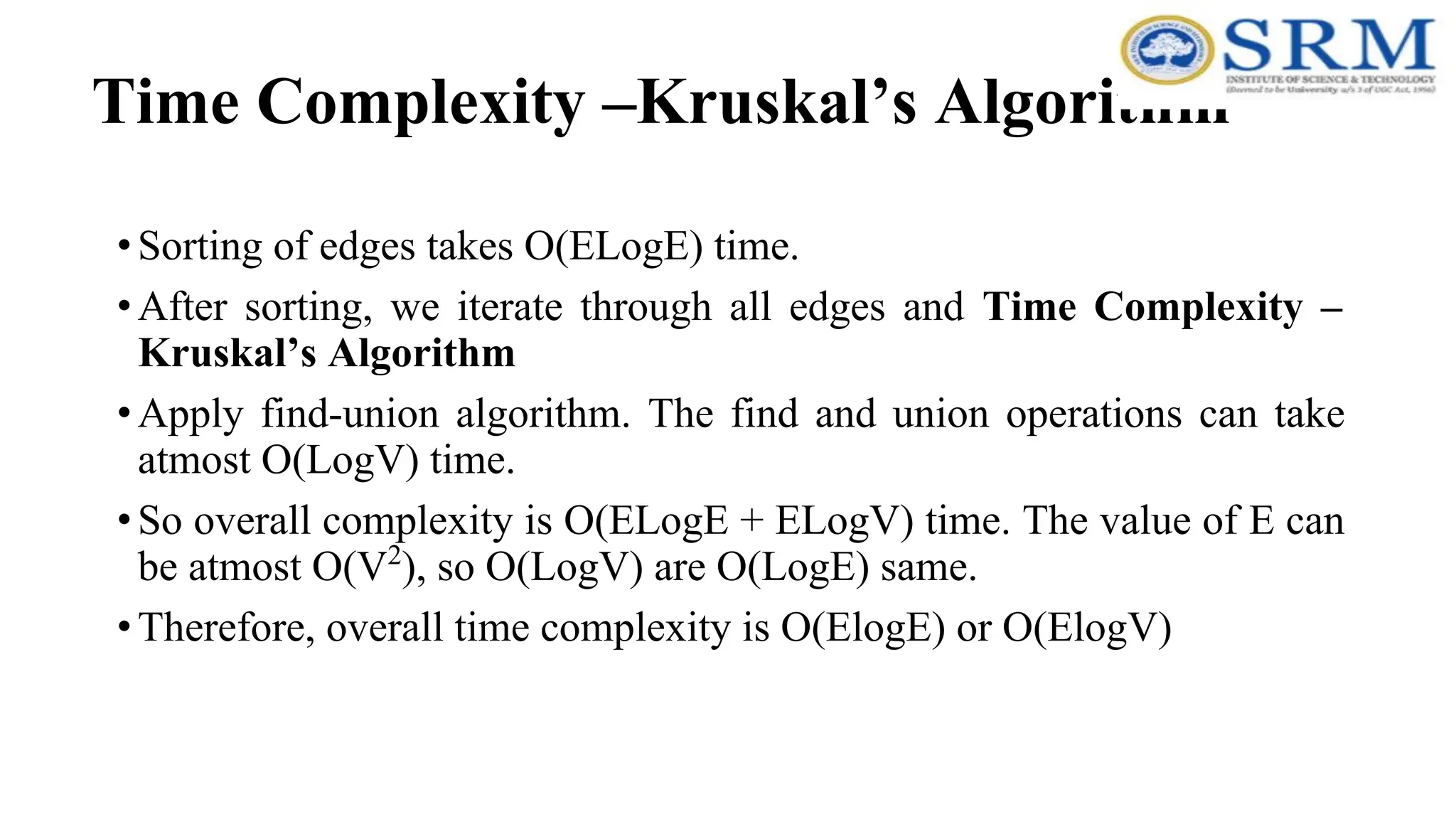
Time Complexity –Kruskal’sAlgorithm •Sorting of edges takes O(ELogE) time. •After sorting, we iterate through all edges and Time Complexity – Kruskal’s Algorithm •Apply find-union algorithm. The find and union operations can take atmost O(LogV) time. •So overall complexity is O(ELogE + ELogV) time. The value of E can be atmost O(V2 ), so O(LogV) are O(LogE) same. •Therefore, overall time complexity is O(ElogE) or O(ElogV)
96.
Real-time Application –Kruskal’s Algorithm •Landing cables •TV Network •Tour Operations •LAN Networks •A network of pipes for drinking water or natural gas. •An electric grid •Single-link Cluster
97.
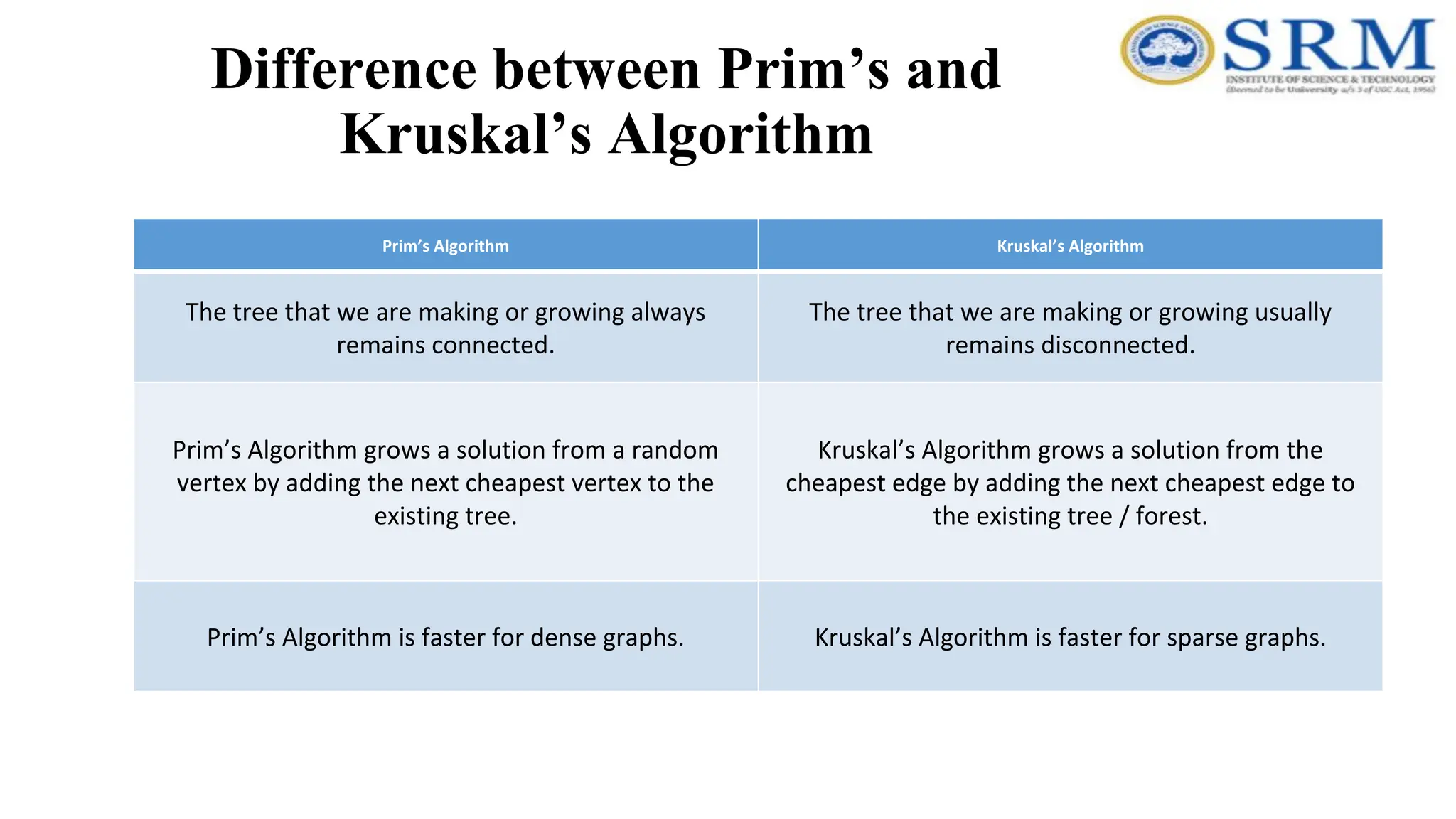
Difference between Prim’sand Kruskal’s Algorithm Prim’s Algorithm Kruskal’s Algorithm The tree that we are making or growing always remains connected. The tree that we are making or growing usually remains disconnected. Prim’s Algorithm grows a solution from a random vertex by adding the next cheapest vertex to the existing tree. Kruskal’s Algorithm grows a solution from the cheapest edge by adding the next cheapest edge to the existing tree / forest. Prim’s Algorithm is faster for dense graphs. Kruskal’s Algorithm is faster for sparse graphs.
98.
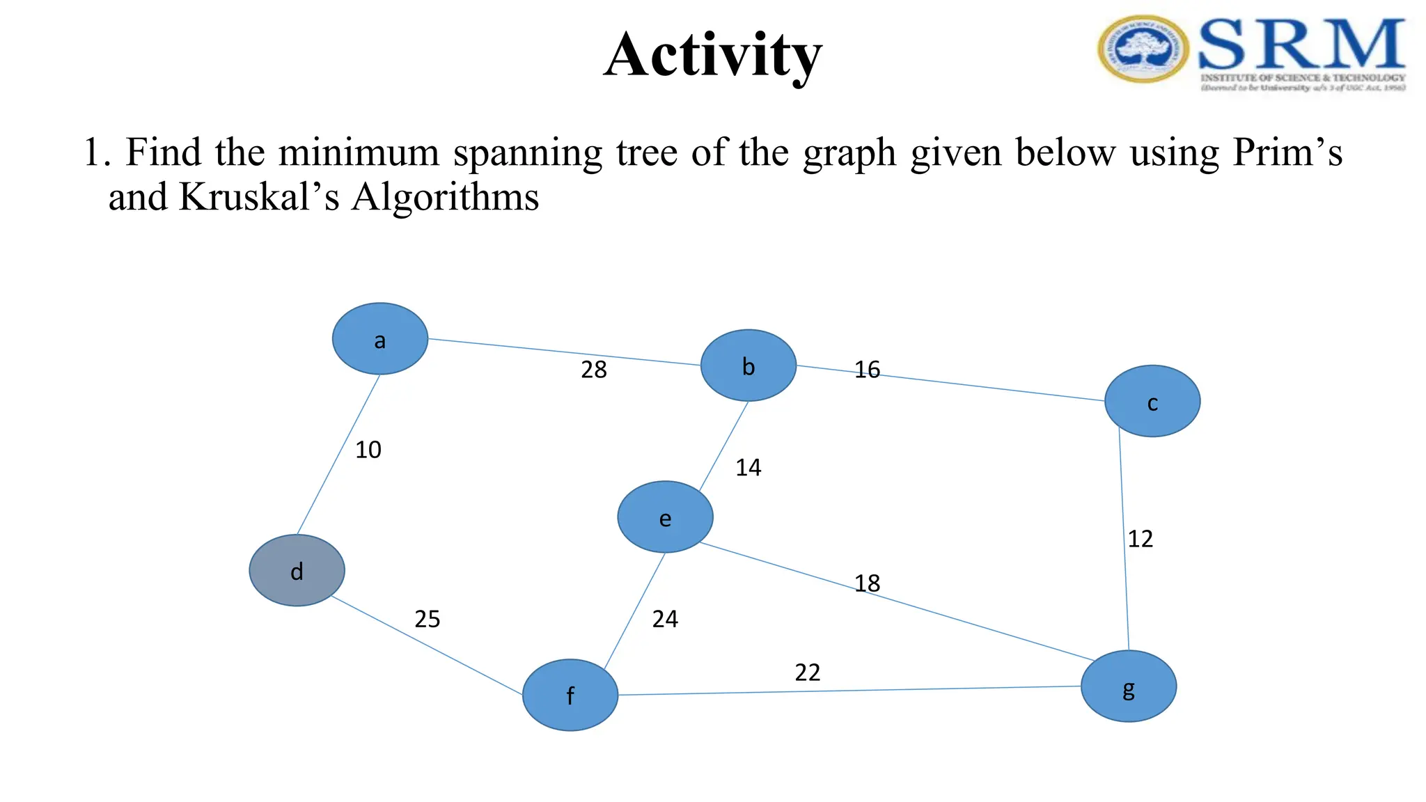
Activity 1. Find theminimum spanning tree of the graph given below using Prim’s and Kruskal’s Algorithms a g c b e f d 10 28 14 12 16 24 25 18 22
99.
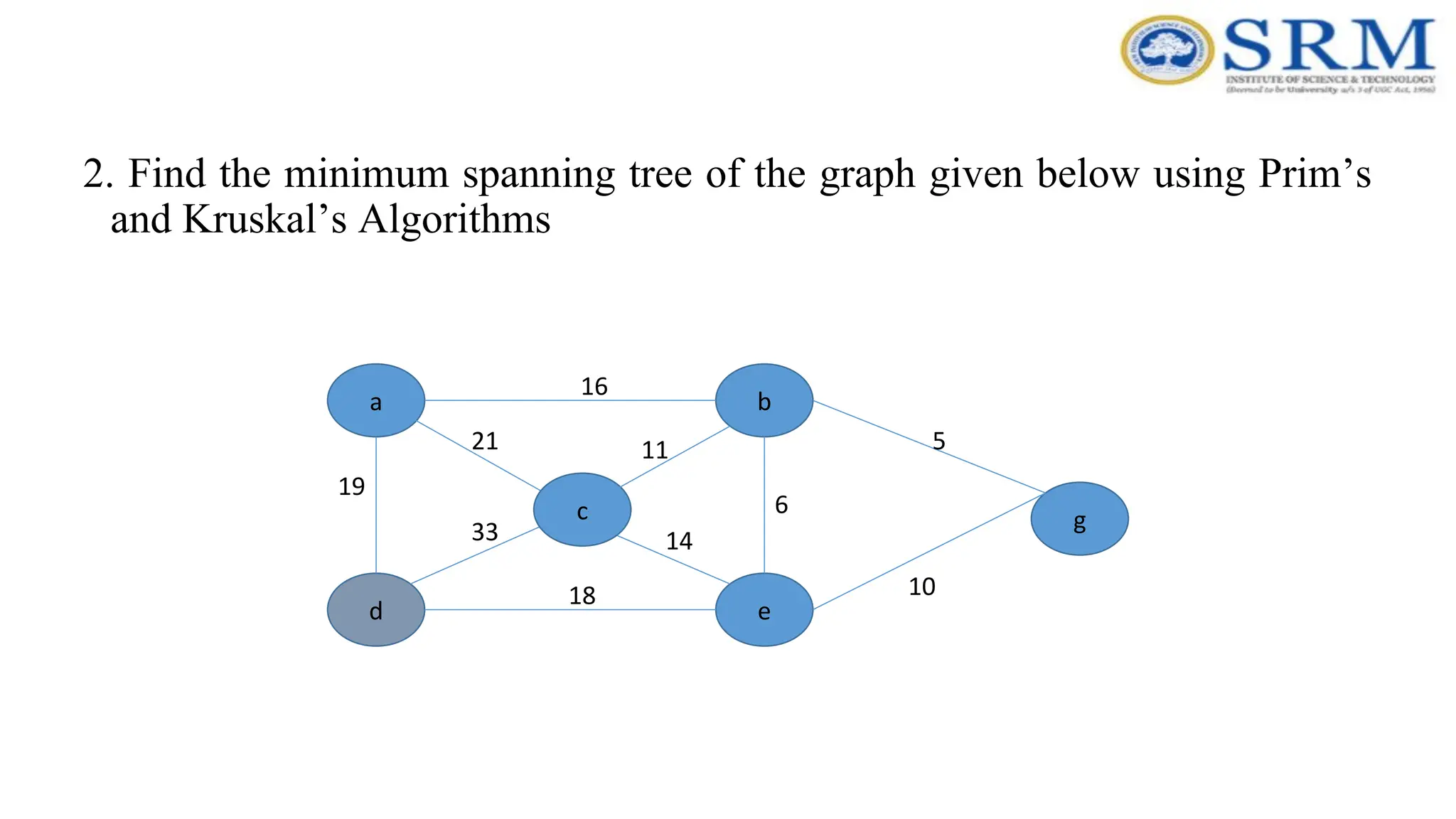
2. Find theminimum spanning tree of the graph given below using Prim’s and Kruskal’s Algorithms a g b e d 19 16 33 6 11 14 18 10 5 c 21
100.
Summary •Both algorithms willalways give solutions with the same length. •They will usually select edges in a different order. •Occasionally they will use different edges – this may happen when you have to choose between edges with the same length.
Introduction to DynamicProgramming Session Learning Outcome-SLO •Critically analyze the different algorithm design techniques for a given problem. •To apply dynamic programming types techniques to solve polynomial time problems.
103.
What is DynamicProgramming? Dynamic programming is a method of solving complex problems by breaking them down into sub-problems that can be solved by working backwards from the last stage. Coined by Richard Bellman who described dynamic programming as the way of solving problems where you need to find the best decisions one after another
104.
Real Time applications 0/1knapsack problem. Mathematical optimization problem. All pair Shortest path problem. Reliability design problem. Longest common subsequence (LCS) Flight control and robotics control. Time sharing: It schedules the job to maximize CPU usage.
105.
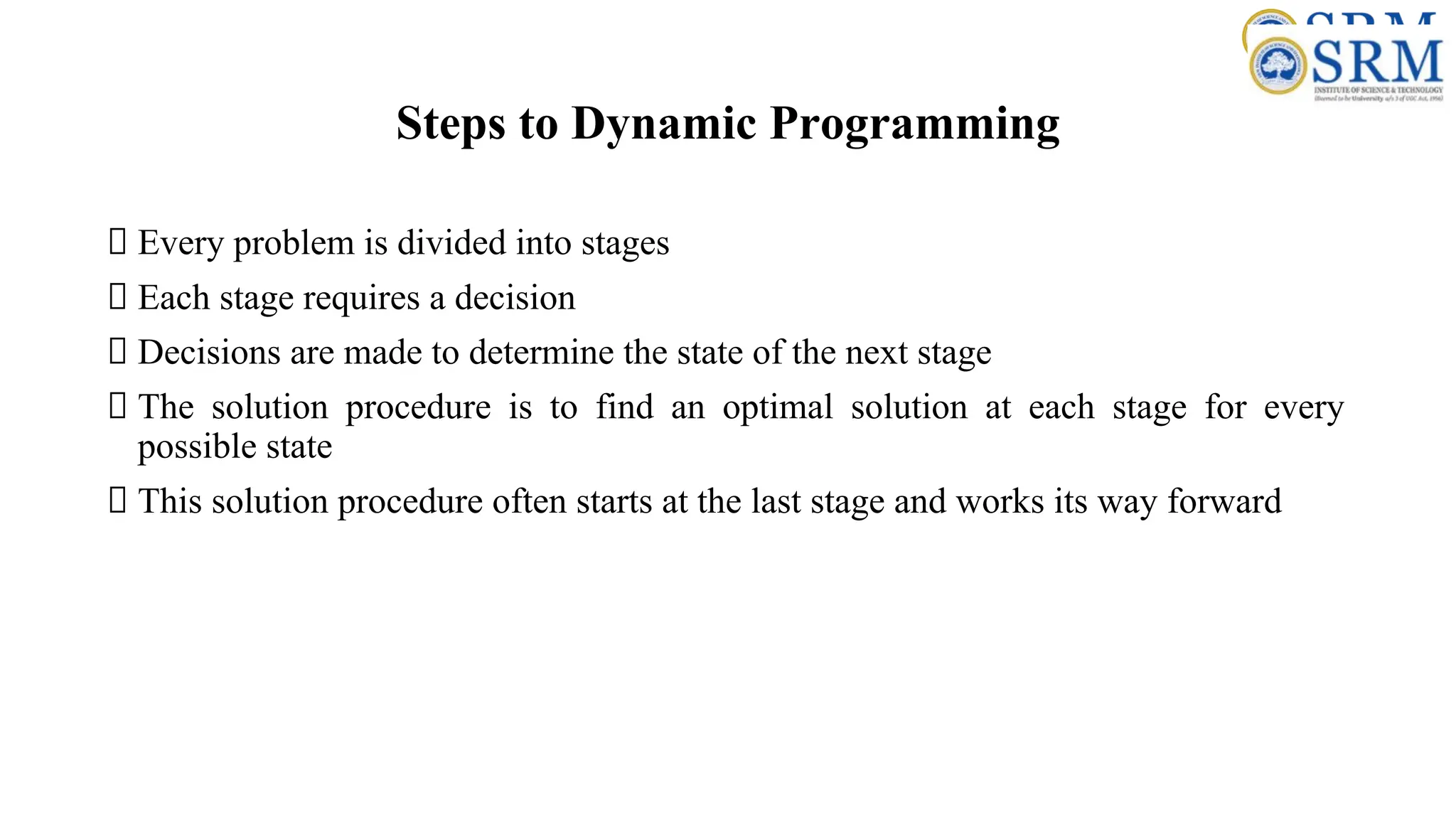
Steps to DynamicProgramming Every problem is divided into stages Each stage requires a decision Decisions are made to determine the state of the next stage The solution procedure is to find an optimal solution at each stage for every possible state This solution procedure often starts at the last stage and works its way forward
106.
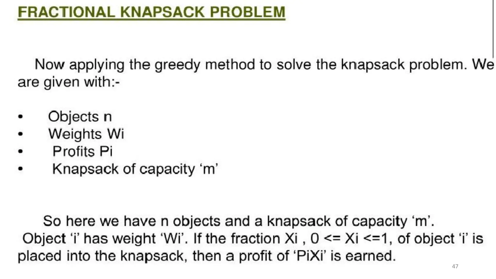
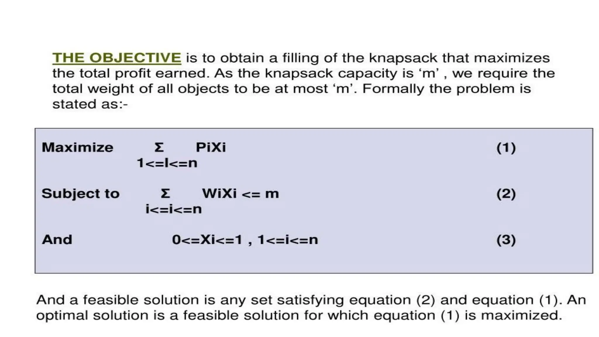
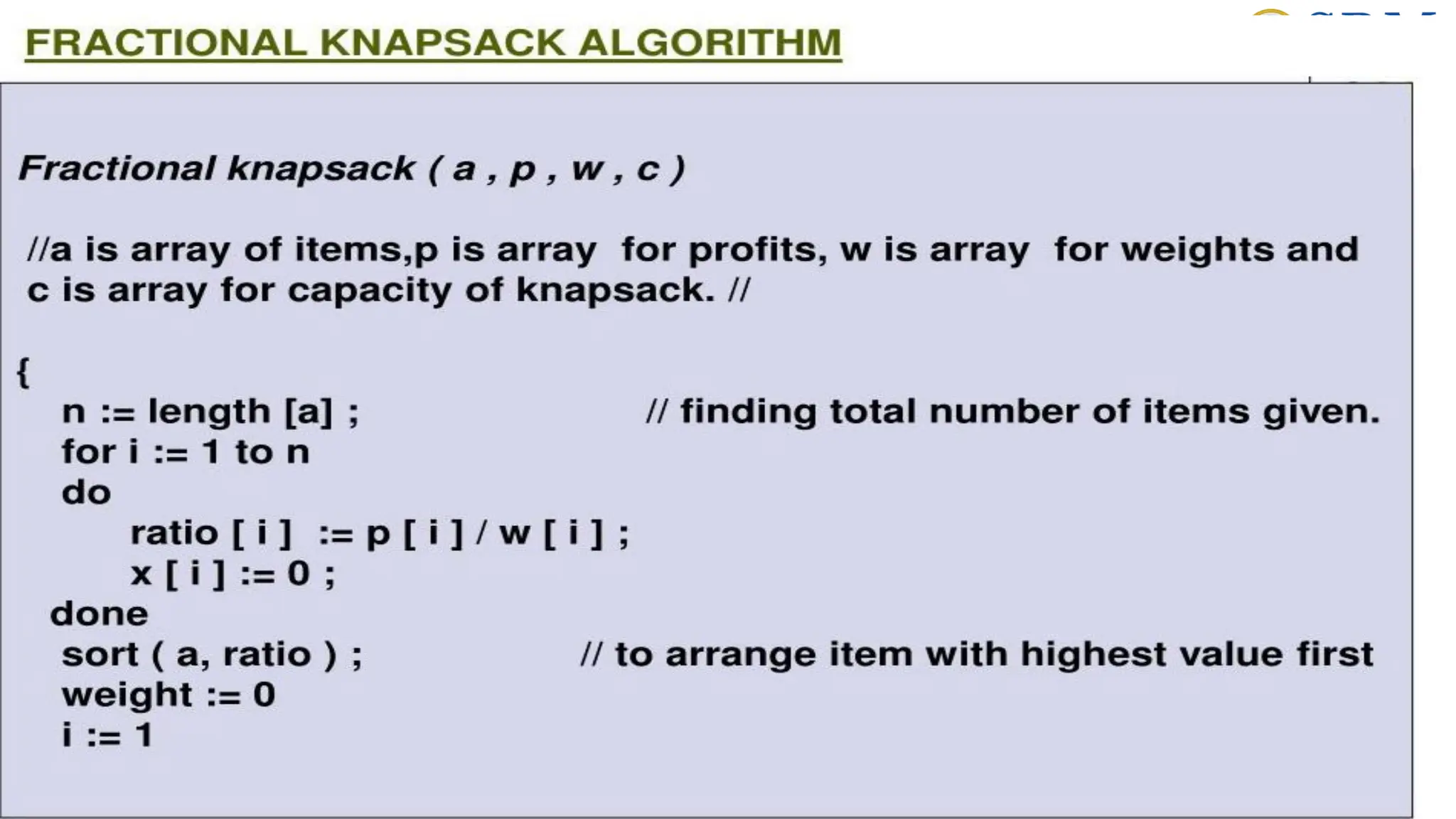
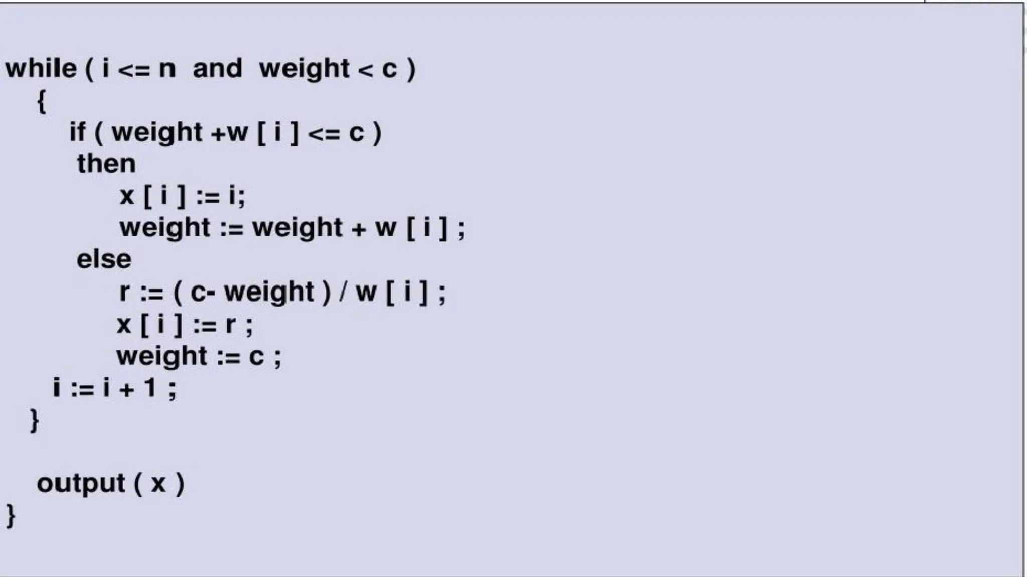
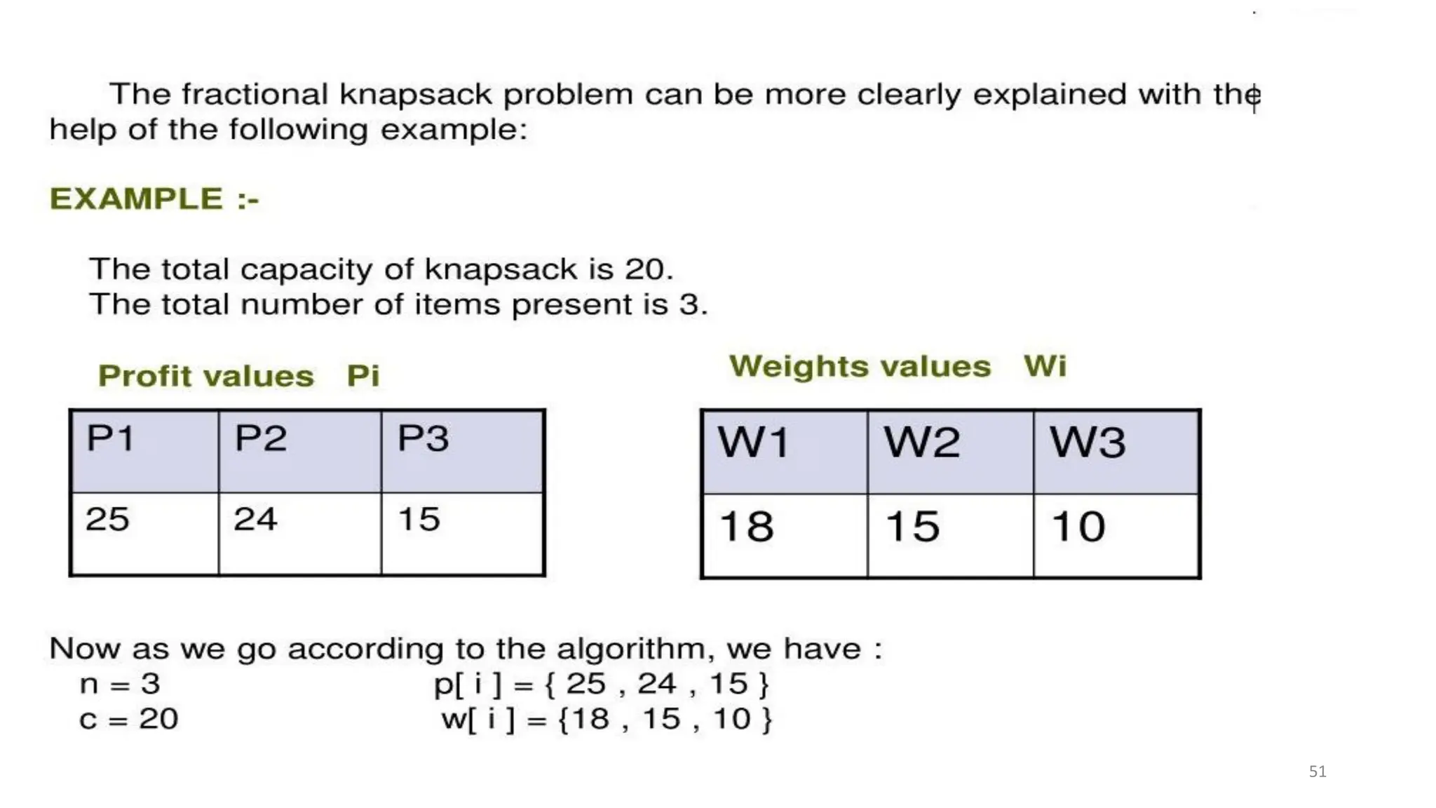
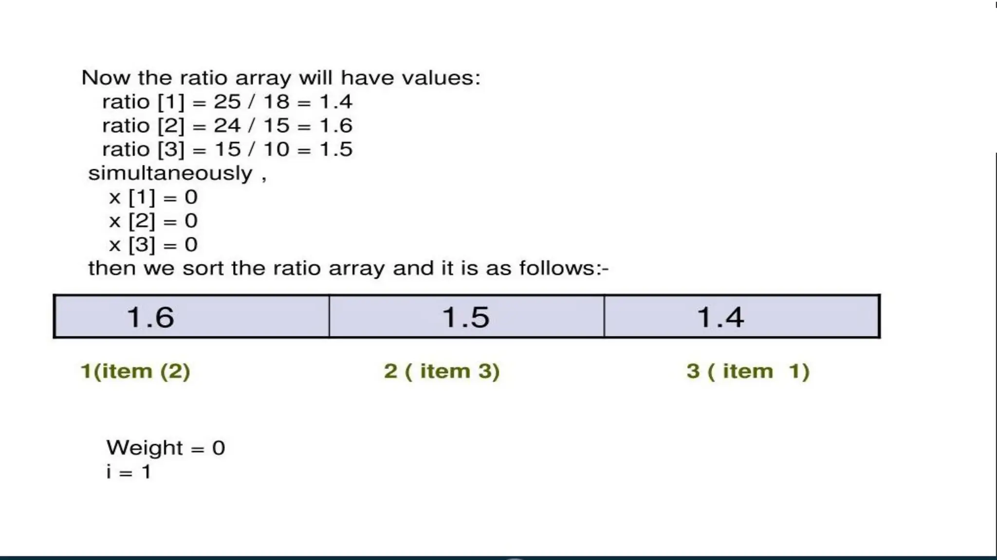
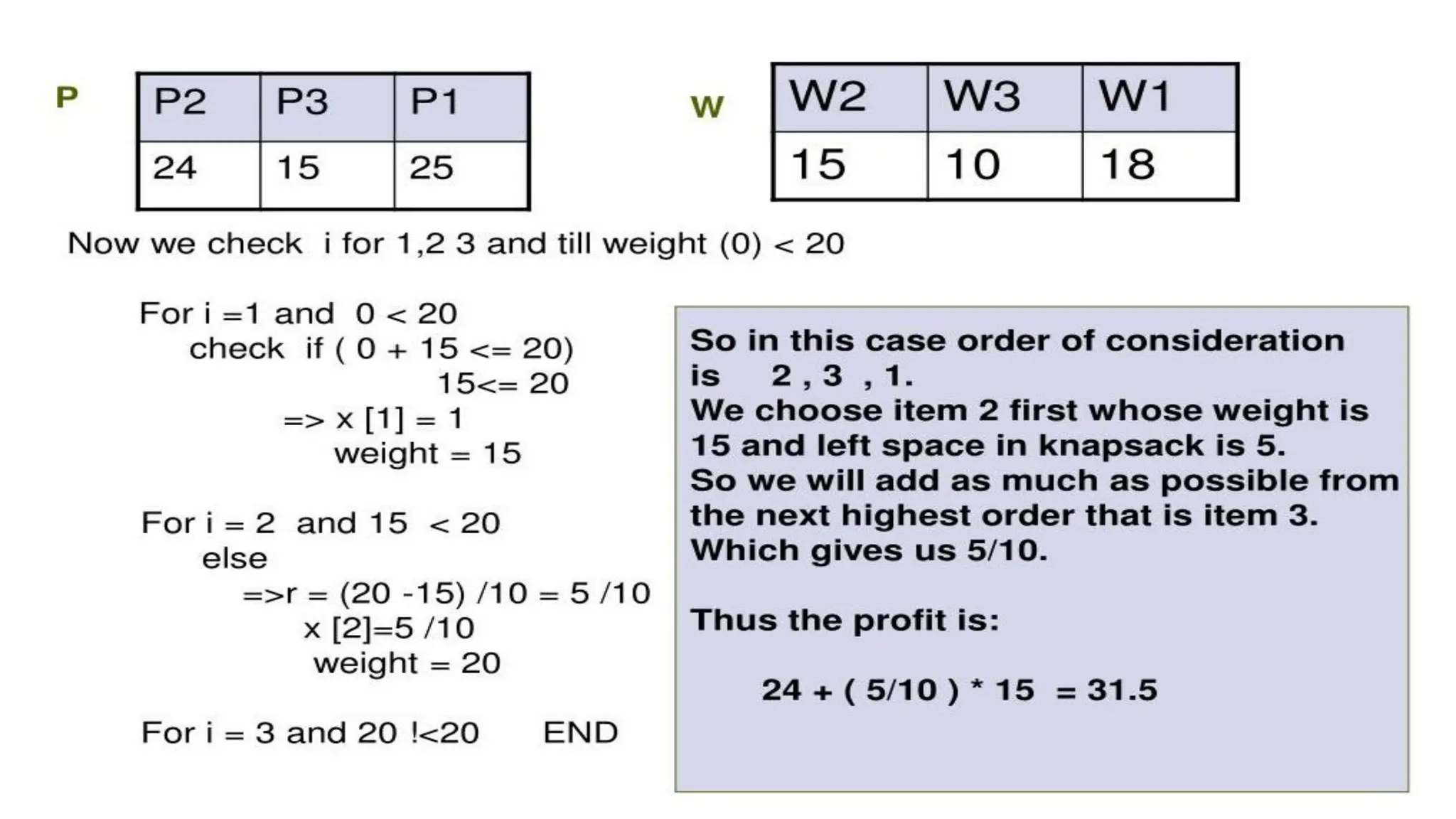
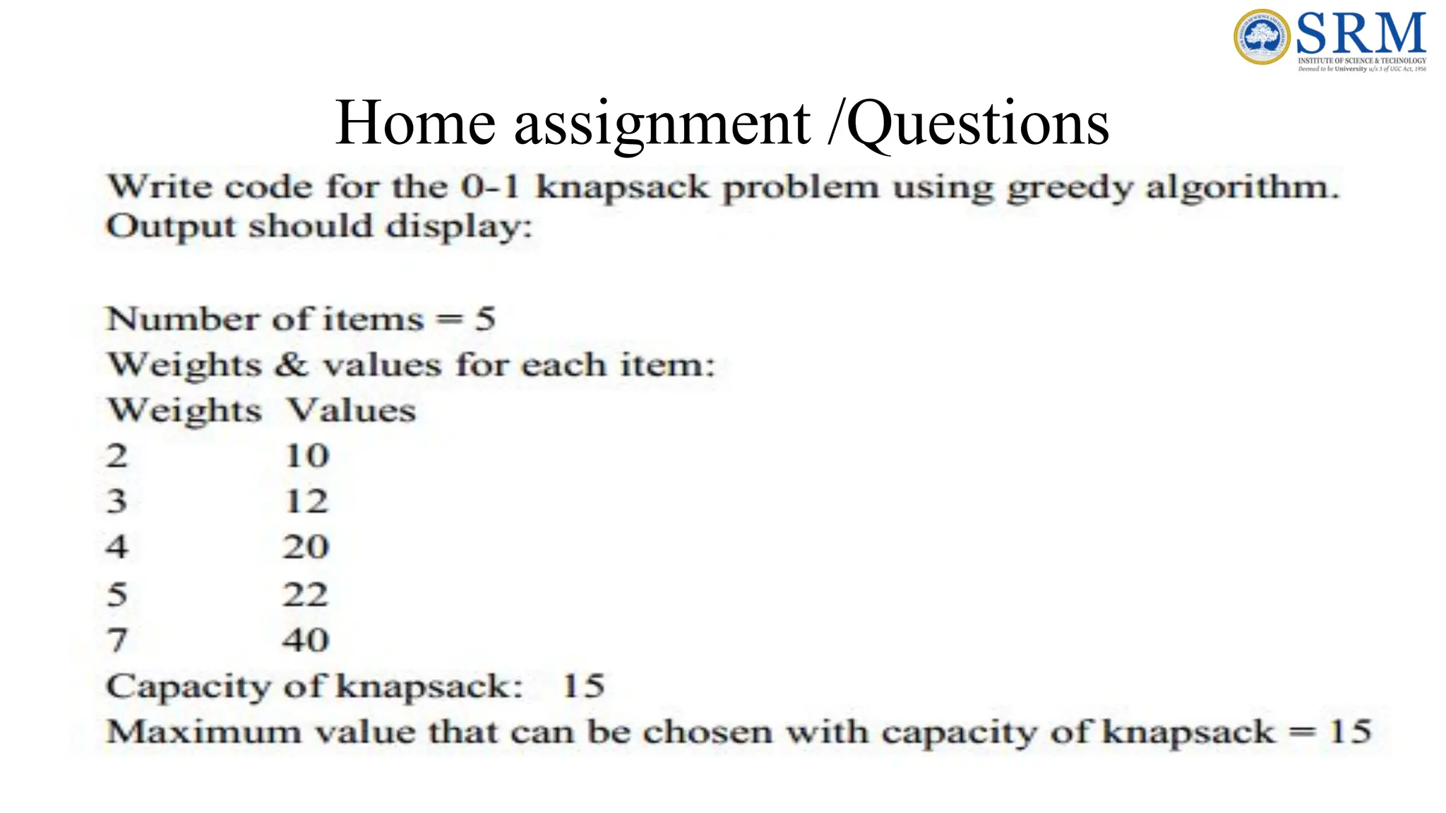
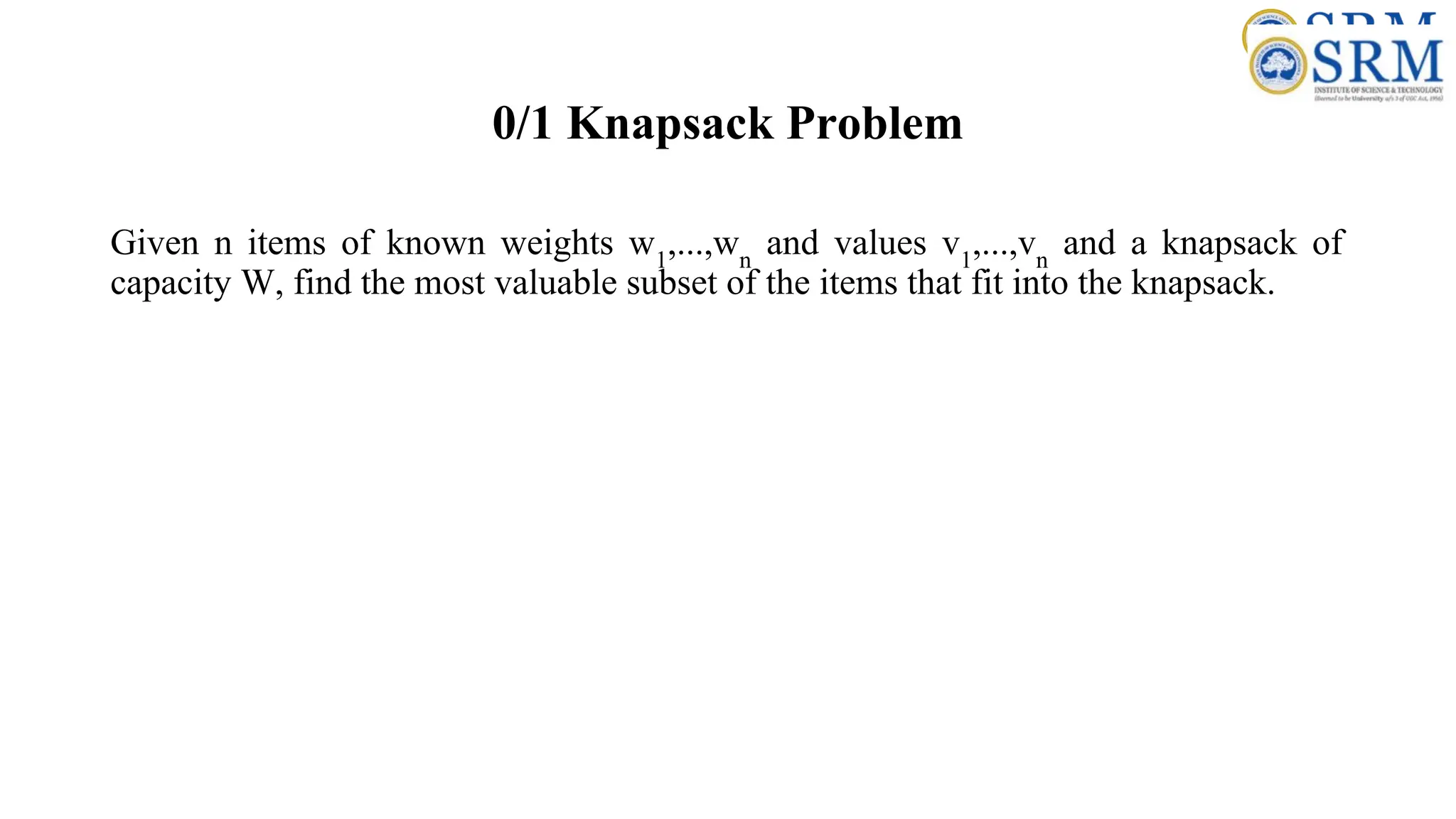
0/1 Knapsack Problem Givenn items of known weights w1 ,...,wn and values v1 ,...,vn and a knapsack of capacity W, find the most valuable subset of the items that fit into the knapsack.
107.
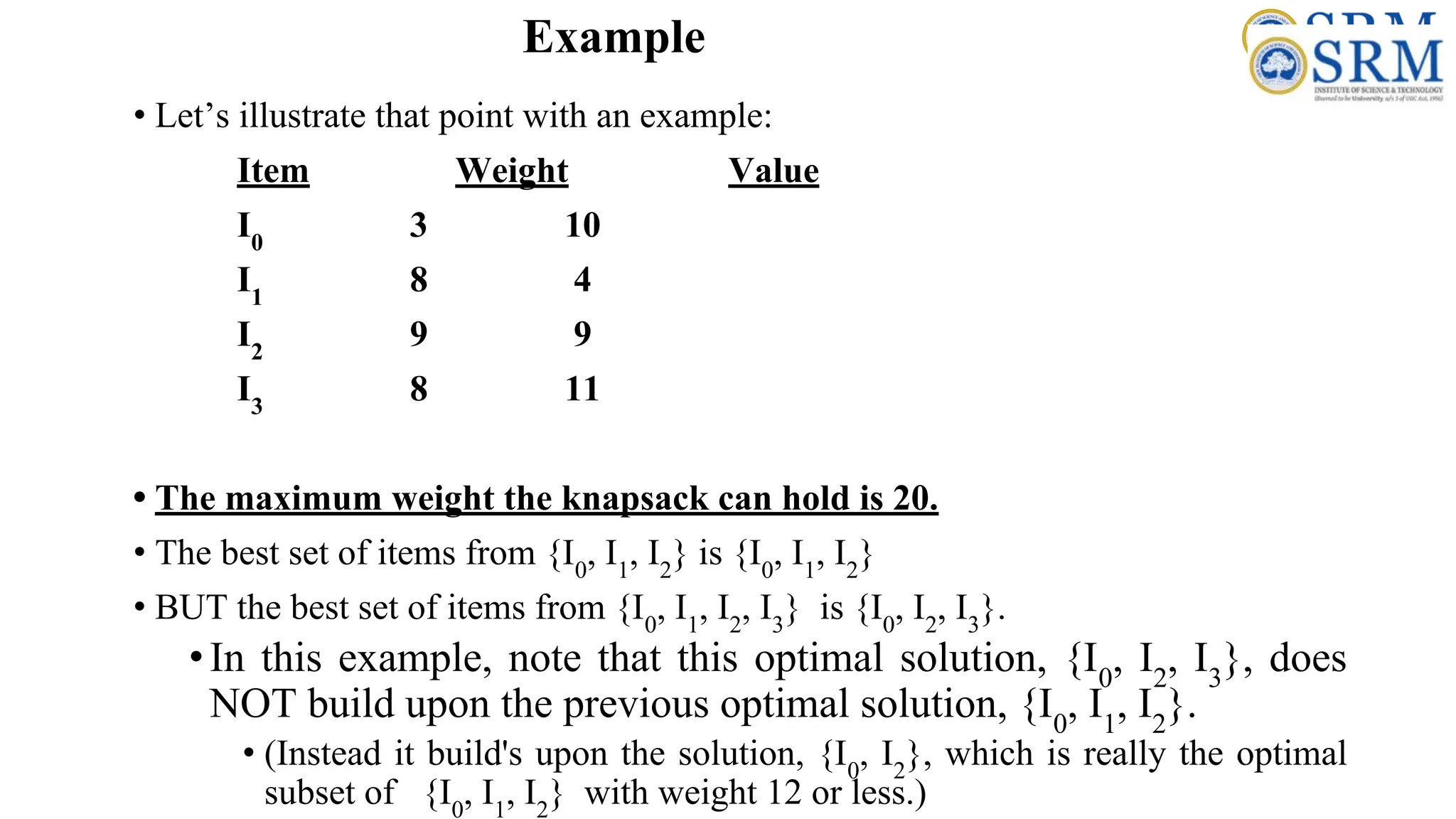
Example • Let’s illustratethat point with an example: Item Weight Value I0 3 10 I1 8 4 I2 9 9 I3 8 11 • The maximum weight the knapsack can hold is 20. • The best set of items from {I0 , I1 , I2 } is {I0 , I1 , I2 } • BUT the best set of items from {I0 , I1 , I2 , I3 } is {I0 , I2 , I3 }. •In this example, note that this optimal solution, {I0 , I2 , I3 }, does NOT build upon the previous optimal solution, {I0 , I1 , I2 }. • (Instead it build's upon the solution, {I0 , I2 }, which is really the optimal subset of {I0 , I1 , I2 } with weight 12 or less.)
108.
Recursive formula • Re-workthe way that builds upon previous sub-problems •Let B[k, w] represent the maximum total value of a subset Sk with weight w. •Our goal is to find B[n, W], where n is the total number of items and W is the maximal weight the knapsack can carry. • Recursive formula for subproblems: B[k, w] = B[k - 1,w], if wk > w = max { B[k - 1,w], B[k - 1,w - wk ] + vk }, otherwise
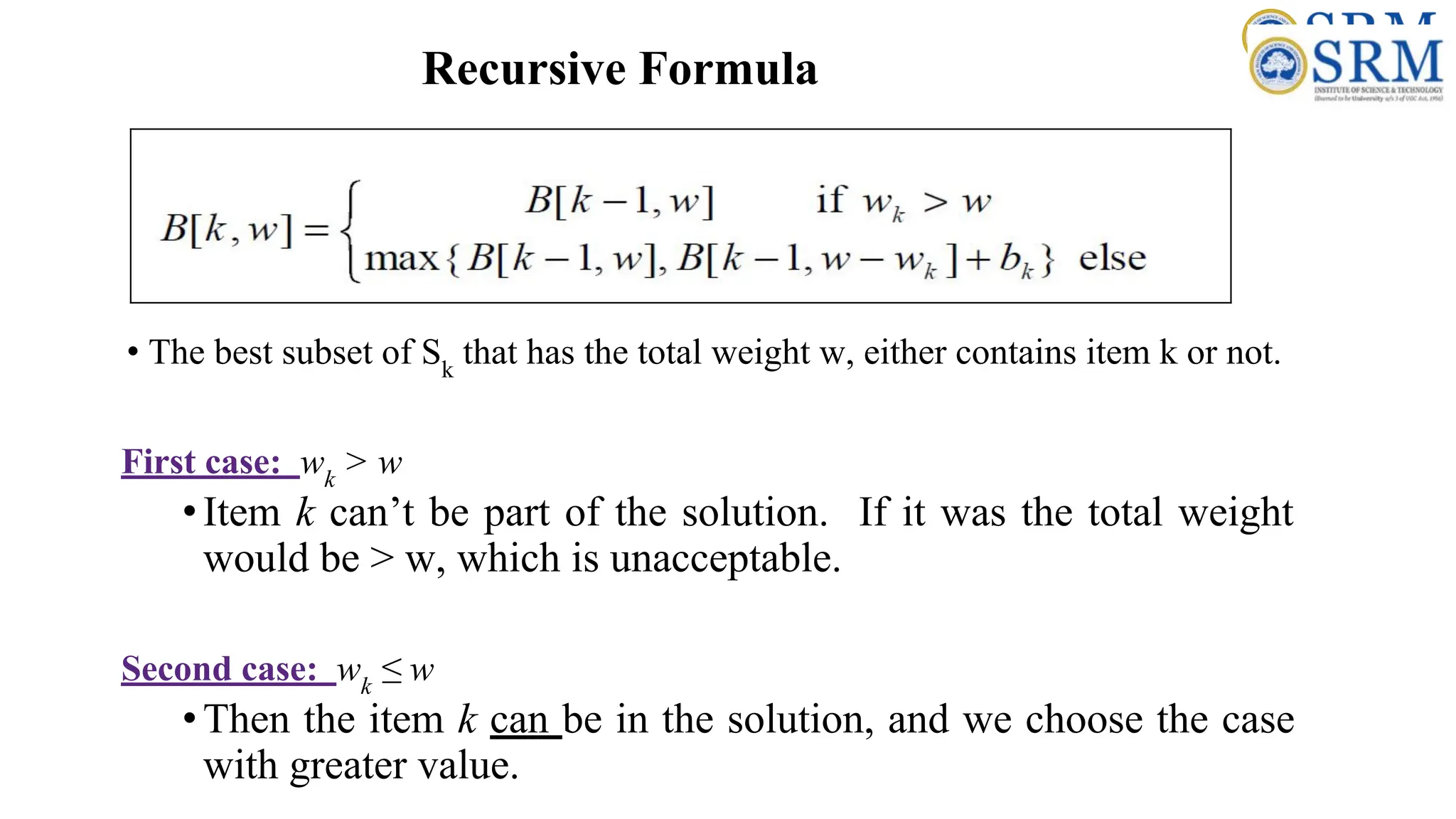
109.
Recursive Formula • Thebest subset of Sk that has the total weight w, either contains item k or not. First case: wk > w •Item k can’t be part of the solution. If it was the total weight would be > w, which is unacceptable. Second case: wk ≤ w •Then the item k can be in the solution, and we choose the case with greater value.
110.
Algorithm for w =0 to W { // Initialize 1st row to 0’s B[0,w] = 0 } for i = 1 to n { // Initialize 1st column to 0’s B[i,0] = 0 } for i = 1 to n { for w = 0 to W { if wi <= w { //item i can be in the solution if vi + B[i-1,w-wi ] > B[i-1,w] B[i,w] = vi + B[i-1,w- wi ] else B[i,w] = B[i-1,w] } else B[i,w] = B[i-1,w] // wi > w } }
111.
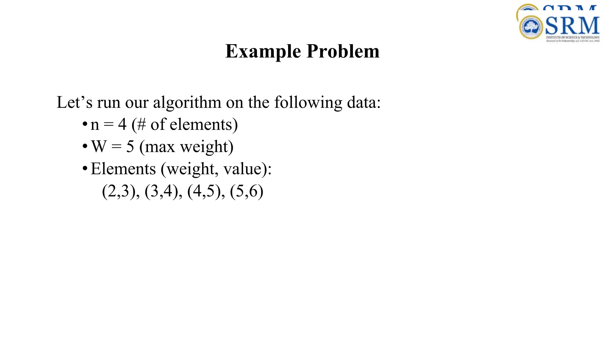
Example Problem Let’s runour algorithm on the following data: •n = 4 (# of elements) •W = 5 (max weight) •Elements (weight, value): (2,3), (3,4), (4,5), (5,6)
112.
Knapsack 0/1 Example i/ w 0 1 2 3 4 5 0 0 0 0 0 0 0 1 0 2 0 3 0 4 0 // Initialize the base cases for w = 0 to W B[0,w] = 0 for i = 1 to n B[i,0] = 0
113.
Knapsack 0/1 Example Items: 1:(2,3) 2: (3,4) 3: (4,5) 4: (5,6) i / w 0 1 2 3 4 5 0 0 0 0 0 0 0 1 0 2 0 3 0 4 0 if wi <= w //item i can be in the solution if vi + B[i-1,w-wi ] > B[i-1,w] B[i,w] = vi + B[i-1,w- wi ] else B[i,w] = B[i-1,w] else B[i,w] = B[i-1,w] // wi > w i = 1 vi = 3 wi = 2 w = 1 w-wi = -1 i / w 0 1 2 3 4 5 0 0 0 0 0 0 0 1 0 0 2 0 3 0 4 0
114.
Knapsack 0/1 Example Items: 1:(2,3) 2: (3,4) 3: (4,5) 4: (5,6) i / w 0 1 2 3 4 5 0 0 0 0 0 0 0 1 0 0 2 0 3 0 4 0 if wi <= w //item i can be in the solution if vi + B[i-1,w-wi ] > B[i-1,w] B[i,w] = vi + B[i-1,w- wi ] else B[i,w] = B[i-1,w] else B[i,w] = B[i-1,w] // wi > w i = 1 vi = 3 wi = 2 w = 2 w-wi = 0 i / w 0 1 2 3 4 5 0 0 0 0 0 0 0 1 0 0 3 2 0 3 0 4 0
115.
Knapsack 0/1 Example Items: 1:(2,3) 2: (3,4) 3: (4,5) 4: (5,6) i / w 0 1 2 3 4 5 0 0 0 0 0 0 0 1 0 0 3 2 0 3 0 4 0 if wi <= w //item i can be in the solution if vi + B[i-1,w-wi ] > B[i-1,w] B[i,w] = vi + B[i-1,w- wi ] else B[i,w] = B[i-1,w] else B[i,w] = B[i-1,w] // wi > w i = 1 vi = 3 wi = 2 w = 3 w-wi = 1 i / w 0 1 2 3 4 5 0 0 0 0 0 0 0 1 0 0 3 3 2 0 3 0 4 0
116.
Knapsack 0/1 Example Items: 1:(2,3) 2: (3,4) 3: (4,5) 4: (5,6) i / w 0 1 2 3 4 5 0 0 0 0 0 0 0 1 0 0 3 3 2 0 3 0 4 0 if wi <= w //item i can be in the solution if vi + B[i-1,w-wi ] > B[i-1,w] B[i,w] = vi + B[i-1,w- wi ] else B[i,w] = B[i-1,w] else B[i,w] = B[i-1,w] // wi > w i = 1 vi = 3 wi = 2 w = 4 w-wi = 2 i / w 0 1 2 3 4 5 0 0 0 0 0 0 0 1 0 0 3 3 3 2 0 3 0 4 0
117.
Knapsack 0/1 Example Items: 1:(2,3) 2: (3,4) 3: (4,5) 4: (5,6) i / w 0 1 2 3 4 5 0 0 0 0 0 0 0 1 0 0 3 3 3 2 0 3 0 4 0 if wi <= w //item i can be in the solution if vi + B[i-1,w-wi ] > B[i-1,w] B[i,w] = vi + B[i-1,w- wi ] else B[i,w] = B[i-1,w] else B[i,w] = B[i-1,w] // wi > w i = 1 vi = 3 wi = 2 w = 5 w-wi = 3 i / w 0 1 2 3 4 5 0 0 0 0 0 0 0 1 0 0 3 3 3 3 2 0 3 0 4 0
118.
Items: 1: (2,3) 2: (3,4) 3:(4,5) 4: (5,6) i / w 0 1 2 3 4 5 0 0 0 0 0 0 0 1 0 0 3 3 3 3 2 0 3 0 4 0 if wi <= w //item i can be in the solution if vi + B[i-1,w-wi ] > B[i-1,w] B[i,w] = vi + B[i-1,w- wi ] else B[i,w] = B[i-1,w] else B[i,w] = B[i-1,w] // wi > w i = 2 vi = 4 wi = 3 w = 1 w-wi = -2 i / w 0 1 2 3 4 5 0 0 0 0 0 0 0 1 0 0 3 3 3 3 2 0 0 3 0 4 0 Knapsack 0/1 Example
119.
Items: 1: (2,3) 2: (3,4) 3:(4,5) 4: (5,6) i / w 0 1 2 3 4 5 0 0 0 0 0 0 0 1 0 0 3 3 3 3 2 0 0 3 0 4 0 if wi <= w //item i can be in the solution if vi + B[i-1,w-wi ] > B[i-1,w] B[i,w] = vi + B[i-1,w- wi ] else B[i,w] = B[i-1,w] else B[i,w] = B[i-1,w] // wi > w i = 2 vi = 4 wi = 3 w = 2 w-wi = -1 i / w 0 1 2 3 4 5 0 0 0 0 0 0 0 1 0 0 3 3 3 3 2 0 0 3 3 0 4 0 Knapsack 0/1 Example
120.
Items: 1: (2,3) 2: (3,4) 3:(4,5) 4: (5,6) i / w 0 1 2 3 4 5 0 0 0 0 0 0 0 1 0 0 3 3 3 3 2 0 0 3 3 0 4 0 if wi <= w //item i can be in the solution if vi + B[i-1,w-wi ] > B[i-1,w] B[i,w] = vi + B[i-1,w- wi ] else B[i,w] = B[i-1,w] else B[i,w] = B[i-1,w] // wi > w i = 2 vi = 4 wi = 3 w = 3 w-wi = 0 i / w 0 1 2 3 4 5 0 0 0 0 0 0 0 1 0 0 3 3 3 3 2 0 0 3 4 3 0 4 0 Knapsack 0/1 Example
121.
Items: 1: (2,3) 2: (3,4) 3:(4,5) 4: (5,6) i / w 0 1 2 3 4 5 0 0 0 0 0 0 0 1 0 0 3 3 3 3 2 0 0 3 4 3 0 4 0 if wi <= w //item i can be in the solution if vi + B[i-1,w-wi ] > B[i-1,w] B[i,w] = vi + B[i-1,w- wi ] else B[i,w] = B[i-1,w] else B[i,w] = B[i-1,w] // wi > w i = 2 vi = 4 wi = 3 w = 4 w-wi = 1 i / w 0 1 2 3 4 5 0 0 0 0 0 0 0 1 0 0 3 3 3 3 2 0 0 3 4 4 3 0 4 0 Knapsack 0/1 Example
122.
Items: 1: (2,3) 2: (3,4) 3:(4,5) 4: (5,6) i / w 0 1 2 3 4 5 0 0 0 0 0 0 0 1 0 0 3 3 3 3 2 0 0 3 4 4 3 0 4 0 if wi <= w //item i can be in the solution if vi + B[i-1,w-wi ] > B[i-1,w] B[i,w] = vi + B[i-1,w- wi ] else B[i,w] = B[i-1,w] else B[i,w] = B[i-1,w] // wi > w i = 2 vi = 4 wi = 3 w = 5 w-wi = 2 i / w 0 1 2 3 4 5 0 0 0 0 0 0 0 1 0 0 3 3 3 3 2 0 0 3 4 4 7 3 0 4 0 Knapsack 0/1 Example
123.
Items: 1: (2,3) 2: (3,4) 3:(4,5) 4: (5,6) i / w 0 1 2 3 4 5 0 0 0 0 0 0 0 1 0 0 3 3 3 3 2 0 0 3 4 4 7 3 0 4 0 if wi <= w //item i can be in the solution if vi + B[i-1,w-wi ] > B[i-1,w] B[i,w] = vi + B[i-1,w- wi ] else B[i,w] = B[i-1,w] else B[i,w] = B[i-1,w] // wi > w i = 3 vi = 5 wi = 4 w = 1..3 w-wi = -3..-1 i / w 0 1 2 3 4 5 0 0 0 0 0 0 0 1 0 0 3 3 3 3 2 0 0 3 4 4 7 3 0 0 3 4 4 0 Knapsack 0/1 Example
124.
Items: 1: (2,3) 2: (3,4) 3:(4,5) 4: (5,6) i / w 0 1 2 3 4 5 0 0 0 0 0 0 0 1 0 0 3 3 3 3 2 0 0 3 4 4 7 3 0 0 3 4 4 0 if wi <= w //item i can be in the solution if vi + B[i-1,w-wi ] > B[i-1,w] B[i,w] = vi + B[i-1,w- wi ] else B[i,w] = B[i-1,w] else B[i,w] = B[i-1,w] // wi > w i = 3 vi = 5 wi = 4 w = 4 w-wi = 0 i / w 0 1 2 3 4 5 0 0 0 0 0 0 0 1 0 0 3 3 3 3 2 0 0 3 4 4 7 3 0 0 3 4 5 4 0 Knapsack 0/1 Example
125.
Items: 1: (2,3) 2: (3,4) 3:(4,5) 4: (5,6) i / w 0 1 2 3 4 5 0 0 0 0 0 0 0 1 0 0 3 3 3 3 2 0 0 3 4 4 7 3 0 0 3 4 5 4 0 if wi <= w //item i can be in the solution if vi + B[i-1,w-wi ] > B[i-1,w] B[i,w] = vi + B[i-1,w- wi ] else B[i,w] = B[i-1,w] else B[i,w] = B[i-1,w] // wi > w i = 3 vi = 5 wi = 4 w = 5 w-wi = 1 i / w 0 1 2 3 4 5 0 0 0 0 0 0 0 1 0 0 3 3 3 3 2 0 0 3 4 4 7 3 0 0 3 4 5 7 4 0 Knapsack 0/1 Example
126.
Items: 1: (2,3) 2: (3,4) 3:(4,5) 4: (5,6) i / w 0 1 2 3 4 5 0 0 0 0 0 0 0 1 0 0 3 3 3 3 2 0 0 3 4 4 7 3 0 0 3 4 5 7 4 0 if wi <= w //item i can be in the solution if vi + B[i-1,w-wi ] > B[i-1,w] B[i,w] = vi + B[i-1,w- wi ] else B[i,w] = B[i-1,w] else B[i,w] = B[i-1,w] // wi > w i = 4 vi = 6 wi = 5 w = 1..4 w-wi = -4..-1 i / w 0 1 2 3 4 5 0 0 0 0 0 0 0 1 0 0 3 3 3 3 2 0 0 3 4 4 7 3 0 0 3 4 5 7 4 0 0 3 4 5 Knapsack 0/1 Example
127.
Items: 1: (2,3) 2: (3,4) 3:(4,5) 4: (5,6) i / w 0 1 2 3 4 5 0 0 0 0 0 0 0 1 0 0 3 3 3 3 2 0 0 3 4 4 7 3 0 0 3 4 5 7 4 0 0 3 4 5 if wi <= w //item i can be in the solution if vi + B[i-1,w-wi ] > B[i-1,w] B[i,w] = vi + B[i-1,w- wi ] else B[i,w] = B[i-1,w] else B[i,w] = B[i-1,w] // wi > w i = 4 vi = 6 wi = 5 w = 5 w-wi = 0 i / w 0 1 2 3 4 5 0 0 0 0 0 0 0 1 0 0 3 3 3 3 2 0 0 3 4 4 7 3 0 0 3 4 5 7 4 0 0 3 4 5 7 Knapsack 0/1 Example
128.
Knapsack 0/1 Example Items: 1:(2,3) 2: (3,4) 3: (4,5) 4: (5,6) i / w 0 1 2 3 4 5 0 0 0 0 0 0 0 1 0 0 3 3 3 3 2 0 0 3 4 4 7 3 0 0 3 4 5 7 4 0 0 3 4 5 7 The max possible value that can be carried in this knapsack is $7
129.
Knapsack 0/1 Algorithm- Finding the Items • This algorithm only finds the max possible value that can be carried in the knapsack •The value in B[n,W] • To know the items that make this maximum value, we need to trace back through the table.
130.
Knapsack 0/1 Algorithm Findingthe Items • Let i = n and k = W if B[i, k] ≠ B[i-1, k] then mark the ith item as in the knapsack i = i-1, k = k-wi else i = i-1 // Assume the ith item is not in the knapsack // Could it be in the optimally packed knapsack?
131.
Finding the Items Items: 1:(2,3) 2: (3,4) 3: (4,5) 4: (5,6) i = 4 k = 5 vi = 6 wi = 5 B[i,k] = 7 B[i-1,k] = 7 i / w 0 1 2 3 4 5 0 0 0 0 0 0 0 1 0 0 3 3 3 3 2 0 0 3 4 4 7 3 0 0 3 4 5 7 4 0 0 3 4 5 7 i = n , k = W while i, k > 0 if B[i, k] ≠ B[i-1, k] then mark the ith item as in the knapsack i = i-1, k = k-wi else i = i-1 Knapsack:
132.
Finding the Items Items: 1:(2,3) 2: (3,4) 3: (4,5) 4: (5,6) i = 3 k = 5 vi = 5 wi = 4 B[i,k] = 7 B[i-1,k] = 7 i / w 0 1 2 3 4 5 0 0 0 0 0 0 0 1 0 0 3 3 3 3 2 0 0 3 4 4 7 3 0 0 3 4 5 7 4 0 0 3 4 5 7 i = n , k = W while i, k > 0 if B[i, k] ≠ B[i-1, k] then mark the ith item as in the knapsack i = i-1, k = k-wi else i = i-1 Knapsack:
133.
Finding the Items Items: 1:(2,3) 2: (3,4) 3: (4,5) 4: (5,6) i = 2 k = 5 vi = 4 wi = 3 B[i,k] = 7 B[i-1,k] = 3 k – wi = 2 i / w 0 1 2 3 4 5 0 0 0 0 0 0 0 1 0 0 3 3 3 3 2 0 0 3 4 4 7 3 0 0 3 4 5 7 4 0 0 3 4 5 7 i = n , k = W while i, k > 0 if B[i, k] ≠ B[i-1, k] then mark the ith item as in the knapsack i = i-1, k = k-wi else i = i-1 Knapsack: Item 2
134.
Finding the Items Items: 1:(2,3) 2: (3,4) 3: (4,5) 4: (5,6) i = 1 k = 2 vi = 3 wi = 2 B[i,k] = 3 B[i-1,k] = 0 k – wi = 0 i / w 0 1 2 3 4 5 0 0 0 0 0 0 0 1 0 0 3 3 3 3 2 0 0 3 4 4 7 3 0 0 3 4 5 7 4 0 0 3 4 5 7 i = n , k = W while i, k > 0 if B[i, k] ≠ B[i-1, k] then mark the ith item as in the knapsack i = i-1, k = k-wi else i = i-1 Knapsack: Item 1 Item 2
135.
Finding the Items Items: 1:(2,3) 2: (3,4) 3: (4,5) 4: (5,6) i = 1 k = 2 vi = 3 wi = 2 B[i,k] = 3 B[i-1,k] = 0 k – wi = 0 i / w 0 1 2 3 4 5 0 0 0 0 0 0 0 1 0 0 3 3 3 3 2 0 0 3 4 4 7 3 0 0 3 4 5 7 4 0 0 3 4 5 7 k = 0, it’s completed The optimal knapsack should contain: Item 1 and Item 2 Knapsack: Item 1 Item 2
136.
Complexity calculation ofknapsack problem for w = 0 to W B[0,w] = 0 for i = 1 to n B[i,0] = 0 for i = 1 to n for w = 0 to W < the rest of the code > What is the running time of this algorithm? O(n*W) O(W) O(W) Repeat n times O(n)
137.
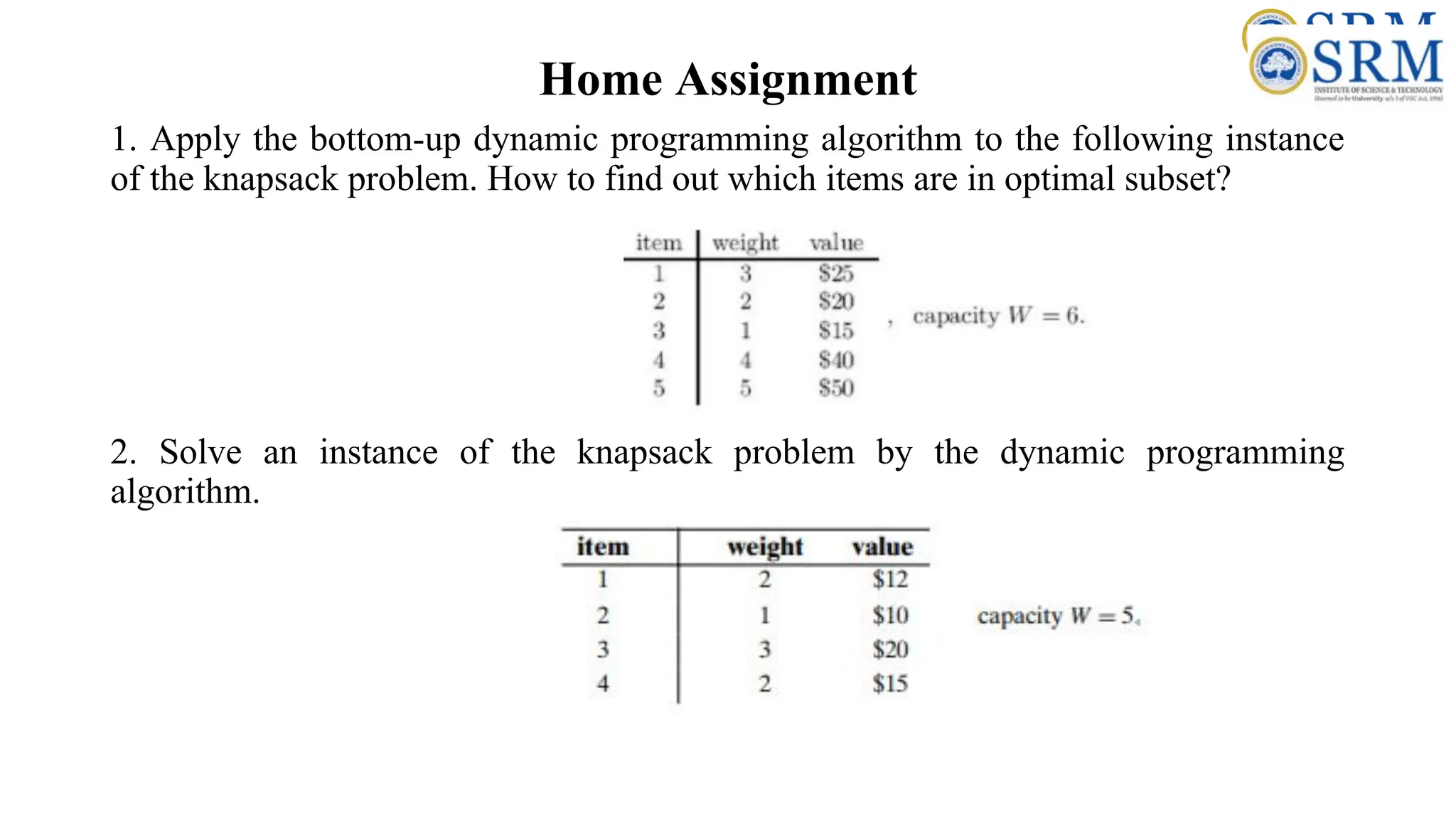
Home Assignment 1. Applythe bottom-up dynamic programming algorithm to the following instance of the knapsack problem. How to find out which items are in optimal subset? 2. Solve an instance of the knapsack problem by the dynamic programming algorithm.
138.
Matrix-chain Multiplication • Supposewe have a sequence or chain A1 , A2 , …, An of n matrices to be multiplied • That is, we want to compute the product A1 A2 …An • There are many possible ways (parenthesizations) to compute the product
139.
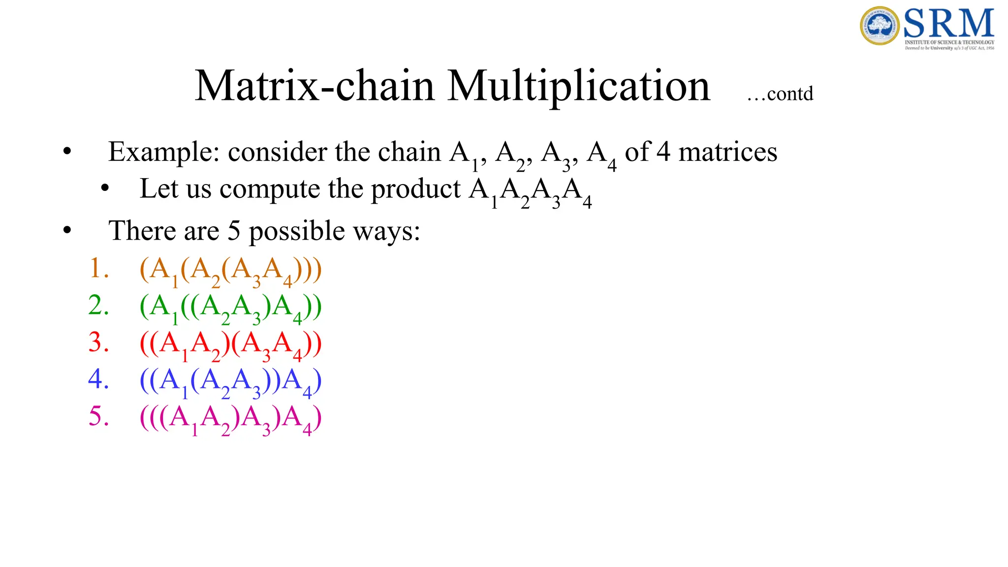
Matrix-chain Multiplication …contd •Example: consider the chain A1 , A2 , A3 , A4 of 4 matrices • Let us compute the product A1 A2 A3 A4 • There are 5 possible ways: 1. (A1 (A2 (A3 A4 ))) 2. (A1 ((A2 A3 )A4 )) 3. ((A1 A2 )(A3 A4 )) 4. ((A1 (A2 A3 ))A4 ) 5. (((A1 A2 )A3 )A4 )
140.
Matrix-chain Multiplication …contd •To compute the number of scalar multiplications necessary, we must know: • Algorithm to multiply two matrices • Matrix dimensions • Can you write the algorithm to multiply two matrices?
141.
Algorithm to Multiply2 Matrices Input: Matrices Ap×q and Bq×r (with dimensions p×q and q×r) Result: Matrix Cp×r resulting from the product A·B MATRIX-MULTIPLY(Ap×q , Bq×r ) 1. for i ← 1 to p 2. for j ← 1 to r 3. C[i, j] ← 0 4. for k ← 1 to q 5. C[i, j] ← C[i, j] + A[i, k] · B[k, j] 6. return C Scalar multiplication in line 5 dominates time to compute CNumber of scalar multiplications = pqr
142.
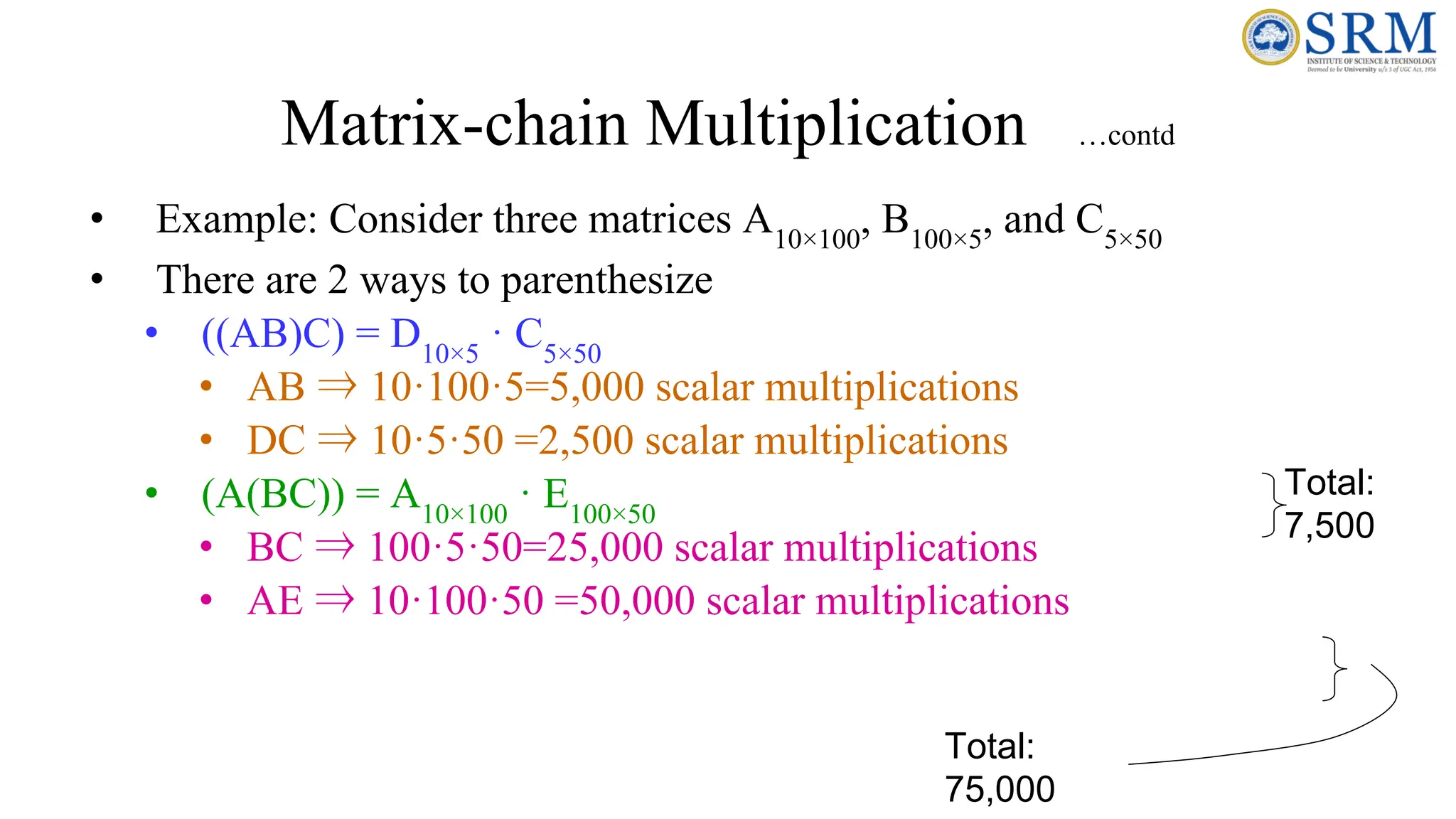
Matrix-chain Multiplication …contd •Example: Consider three matrices A10×100 , B100×5 , and C5×50 • There are 2 ways to parenthesize • ((AB)C) = D10×5 · C5×50 • AB ⇒ 10·100·5=5,000 scalar multiplications • DC ⇒ 10·5·50 =2,500 scalar multiplications • (A(BC)) = A10×100 · E100×50 • BC ⇒ 100·5·50=25,000 scalar multiplications • AE ⇒ 10·100·50 =50,000 scalar multiplications Total: 7,500 Total: 75,000
143.
Matrix-chain Multiplication …contd •Matrix-chain multiplication problem • Given a chain A1 , A2 , …, An of n matrices, where for i=1, 2, …, n, matrix Ai has dimension pi-1 ×pi • Parenthesize the product A1 A2 …An such that the total number of scalar multiplications is minimized • Brute force method of exhaustive search takes time exponential in n
144.
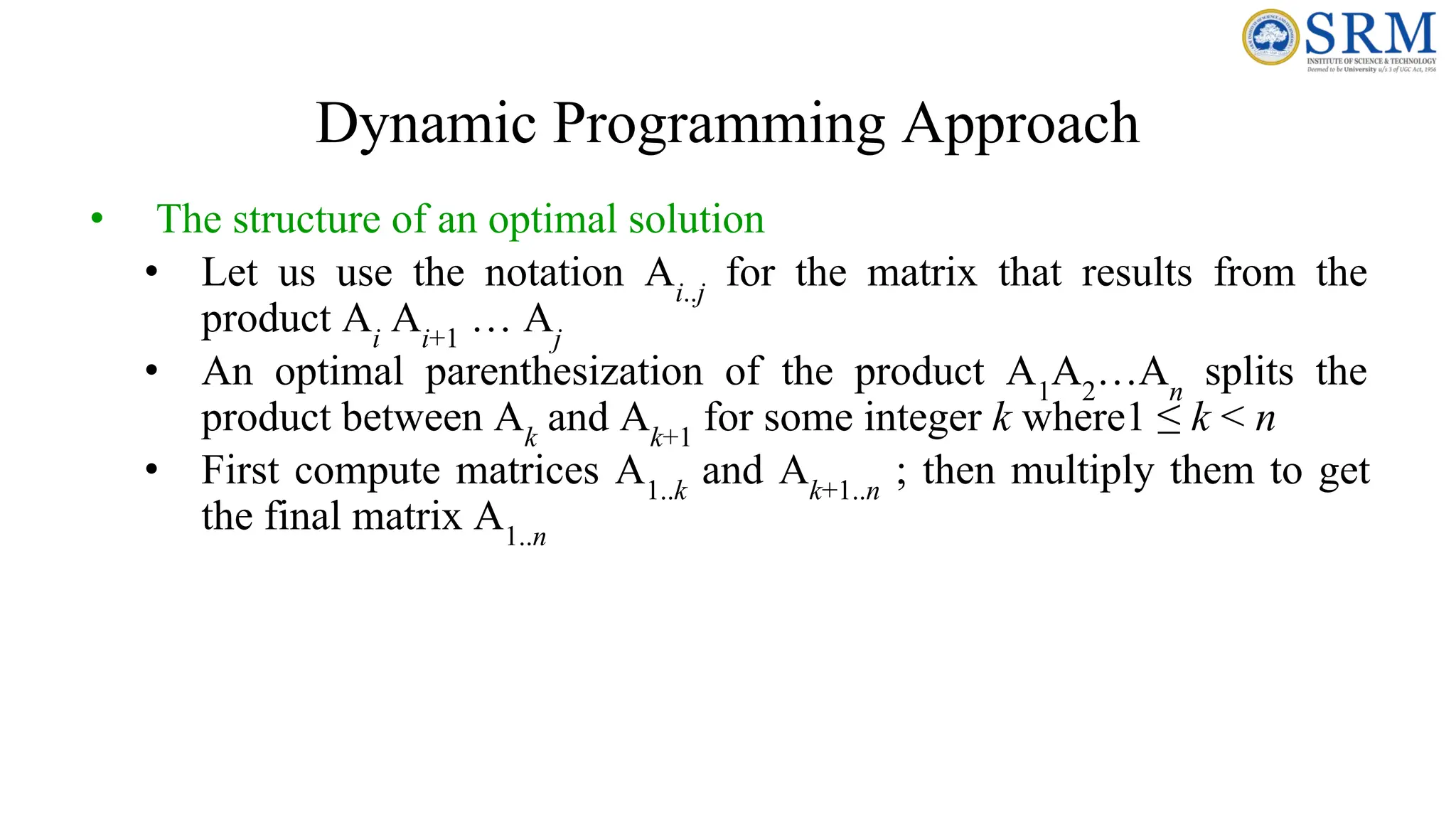
Dynamic Programming Approach •The structure of an optimal solution • Let us use the notation Ai..j for the matrix that results from the product Ai Ai+1 … Aj • An optimal parenthesization of the product A1 A2 …An splits the product between Ak and Ak+1 for some integer k where1 ≤ k < n • First compute matrices A1..k and Ak+1..n ; then multiply them to get the final matrix A1..n
145.
Dynamic Programming Approach…contd • Key observation: parenthesizations of the subchains A1 A2 …Ak and Ak+1 Ak+2 …An must also be optimal if the parenthesization of the chain A1 A2 …An is optimal (why?) • That is, the optimal solution to the problem contains within it the optimal solution to subproblems
146.
Dynamic Programming Approach…contd • Recursive definition of the value of an optimal solution • Let m[i, j] be the minimum number of scalar multiplications necessary to compute Ai..j • Minimum cost to compute A1..n is m[1, n] • Suppose the optimal parenthesization of Ai..j splits the product between Ak and Ak+1 for some integer k where i ≤ k < j
147.
Dynamic Programming Approach…contd • Ai..j = (Ai Ai+1 …Ak )·(Ak+1 Ak+2 …Aj )= Ai..k · Ak+1..j • Cost of computing Ai..j = cost of computing Ai..k + cost of computing Ak+1..j + cost of multiplying Ai..k and Ak+1..j • Cost of multiplying Ai..k and Ak+1..j is pi-1 pk pj • m[i, j ] = m[i, k] + m[k+1, j ] + pi-1 pk pj for i ≤ k < j • m[i, i ] = 0 for i=1,2,…,n
148.
Dynamic Programming Approach…contd • But… optimal parenthesization occurs at one value of k among all possible i ≤ k < j • Check all these and select the best one m[i, j ] = 0 if i=j min {m[i, k] + m[k+1, j ] + pi-1 pk pj } if i<j i ≤ k< j
149.
Dynamic Programming Approach…contd • To keep track of how to construct an optimal solution, we use a table s • s[i, j ] = value of k at which Ai Ai+1 … Aj is split for optimal parenthesization • Algorithm: next slide • First computes costs for chains of length l=1 • Then for chains of length l=2,3, … and so on • Computes the optimal cost bottom-up
150.
Algorithm to ComputeOptimal Cost Input: Array p[0…n] containing matrix dimensions and n Result: Minimum-cost table m and split table s MATRIX-CHAIN-ORDER(p[ ], n) for i ← 1 to n m[i, i] ← 0 for l ← 2 to n for i ← 1 to n-l+1 j ← i+l-1 m[i, j] ← ∞ for k ← i to j-1 q ← m[i, k] + m[k+1, j] + p[i-1] p[k] p[j] if q < m[i, j] m[i, j] ← q s[i, j] ← k return m and s Takes O(n3 ) time Requires O(n2 ) space
151.
Constructing Optimal Solution •Our algorithm computes the minimum-cost table m and the split table s • The optimal solution can be constructed from the split table s • Each entry s[i, j ]=k shows where to split the product Ai Ai+1 … Aj for the minimum cost
152.
Example • Show howto multiply this matrix chain optimally • Solution on the board • Minimum cost 15,125 • Optimal parenthesization ((A1 (A2 A3 ))((A4 A5 )A6 )) Matrix Dimension A1 30×35 A2 35×15 A3 15×5 A4 5×10 A5 10×20 A6 20×25
LCS using DynamicProgramming •SLO 1: To understand the Longest Common Subsequence(LCS) Problem and how it can be solved using Dynamic programming approach.
Example •A subsequence isa sequence that appears in the same relative order, but not necessarily contiguous. •Let String S1= a b c d •Subsequence •Length of LCS=4 •Subsequence : abcd ab bd ca ac ad db ba acd bcd abcd
157.
LCS Example •S1= ab c d e f g h i j •S2= c d g i •Subsequence •S1: •S2: •Subsequence, SS1: c d g i a b c d e f g h i j c d g i
158.
Example •S1= a bc d e f g h i j •S2= c d g i •Subsequence •S1: •S2: •Subsequence, SS2: d g i a b c d e f g h i j c d g i
159.
Example •S1= a bc d e f g h i j •S2= c d g i •Subsequence •S1: •S2: •Subsequence, SS3: g i a b c d e f g h i j c d g i
160.
Example •SS1= c dg i •SS2: d g i •SS3: g i • Longest Common Subsequence: subsequence with maximum length. maximum(length(subsequence1), length(subsequence2)…. length(subsequence n)). Longest Common Subsequence : maximum(length(c d g i), length(d g i),length(g i)). •Therefore LCS (S1,S2) is c d g i with length 4
Motivation Brute Force Approach-Checkevery subsequence of x[1 . . m] to see if it is also a subsequence of y[1 . . n]. Analysis • 2m subsequences of x (each bit-vector of length m determines a distinct subsequence of x). • Hence, the runtime would be exponential ! Example: Consider S1 = ACCGGTCGAGTGCGCGGAAGCCGGCCGAA….. S2 = GTCGTTCGGAATGCCGTTGCTCTGTAAA…. Towards a better algorithm: a Dynamic Prpgramming strategy • Key: optimal substructure and overlapping sub-problems • First we’ll find the length of LCS. Later we’ll modify the algorithm to find LCS itself.
163.
LCS Problem Formulationusing DP Algorithm • Key: find out the correct order to solve the sub-problems • Total number of sub-problems: m * n c[i, j] = c[i–1, j–1] + 1 if x[i] = y[j], max{c[i–1, j], c[i, j–1]} otherwise. C(i, j) 0 m 0 n i j
164.
LCS Example We’ll seehow LCS algorithm works on the following example: •X = ABCB •Y = BDCAB LCS(X, Y) = BCB X = A B C B Y = B D C A B What is the LCS of X and Y?
LCS Example (0) j0 1 2 3 4 5 0 1 2 3 4 i X[i] A B C B Y[j] B B A C D X = ABCB; m = |X| = 4 Y = BDCAB; n = |Y| = 5 Allocate array c[5,6] ABCB BDCAB
167.
LCS Example (1) j0 1 2 3 4 5 0 1 2 3 4 i A B C B B B A C D 0 0 0 0 0 0 0 0 0 0 for i = 1 to m c[i,0] = 0 for j = 1 to n c[0,j] = 0 ABCB BDCAB X[i] Y[j]
168.
LCS Example (2) j0 1 2 3 4 5 0 1 2 3 4 i A B C B B B A C D 0 0 0 0 0 0 0 0 0 0 if ( Xi == Yj ) c[i,j] = c[i-1,j-1] + 1 else c[i,j] = max( c[i-1,j], c[i,j-1] ) 0 ABCB BDCAB X[i] Y[j]
169.
LCS Example (3) j0 1 2 3 4 5 0 1 2 3 4 i A B C B B B A C D 0 0 0 0 0 0 0 0 0 0 if ( Xi == Yj ) c[i,j] = c[i-1,j-1] + 1 else c[i,j] = max( c[i-1,j], c[i,j-1] ) 0 0 0 ABCB BDCAB X[i] Y[j]
170.
LCS Example (4) j0 1 2 3 4 5 0 1 2 3 4 i A B C B B B A C D 0 0 0 0 0 0 0 0 0 0 if ( Xi == Yj ) c[i,j] = c[i-1,j-1] + 1 else c[i,j] = max( c[i-1,j], c[i,j-1] ) 0 0 0 1 ABCB BDCAB X[i] Y[j]
171.
LCS Example (5) j0 1 2 3 4 5 0 1 2 3 4 i A B C B B B A C D 0 0 0 0 0 0 0 0 0 0 if ( Xi == Yj ) c[i,j] = c[i-1,j-1] + 1 else c[i,j] = max( c[i-1,j], c[i,j-1] ) 0 0 0 1 1 ABCB BDCAB X[i] Y[j]
172.
LCS Example (6) j0 1 2 3 4 5 0 1 2 3 4 i A B C B B B A C D 0 0 0 0 0 0 0 0 0 0 if ( Xi == Yj ) c[i,j] = c[i-1,j-1] + 1 else c[i,j] = max( c[i-1,j], c[i,j-1] ) 0 0 1 0 1 1 ABCB BDCAB X[i] Y[j]
173.
LCS Example (7) j0 1 2 3 4 5 0 1 2 3 4 i A B C B B B A C D 0 0 0 0 0 0 0 0 0 0 if ( Xi == Yj ) c[i,j] = c[i-1,j-1] + 1 else c[i,j] = max( c[i-1,j], c[i,j-1] ) 1 0 0 0 1 1 1 1 1 ABCB BDCAB X[i] Y[j]
174.
LCS Example (8) j0 1 2 3 4 5 0 1 2 3 4 i A B C B B B A C D 0 0 0 0 0 0 0 0 0 0 if ( Xi == Yj ) c[i,j] = c[i-1,j-1] + 1 else c[i,j] = max( c[i-1,j], c[i,j-1] ) 1 0 0 0 1 1 1 1 1 2 ABCB BDCAB X[i] Y[j]
175.
LCS Example (9) j0 1 2 3 4 5 0 1 2 3 4 i A B C B B B A C D 0 0 0 0 0 0 0 0 0 0 if ( Xi == Yj ) c[i,j] = c[i-1,j-1] + 1 else c[i,j] = max( c[i-1,j], c[i,j-1] ) 1 0 0 0 1 2 1 1 1 1 1 1 ABCB BDCAB X[i] Y[j]
176.
LCS Example (10) j0 1 2 3 4 5 0 1 2 3 4 i A B C B B B A C D 0 0 0 0 0 0 0 0 0 0 if ( Xi == Yj ) c[i,j] = c[i-1,j-1] + 1 else c[i,j] = max( c[i-1,j], c[i,j-1] ) 1 0 0 0 1 1 2 1 1 1 1 1 2 ABCB BDCAB X[i] Y[j]
177.
LCS Example (11) j0 1 2 3 4 5 0 1 2 3 4 i A B C B B B A C D 0 0 0 0 0 0 0 0 0 0 if ( Xi == Yj ) c[i,j] = c[i-1,j-1] + 1 else c[i,j] = max( c[i-1,j], c[i,j-1] ) 1 0 0 0 1 1 2 1 1 1 1 2 1 2 2 ABCB BDCAB X[i] Y[j]
178.
LCS Example (12) j0 1 2 3 4 5 0 1 2 3 4 i A B C B B B A C D 0 0 0 0 0 0 0 0 0 0 if ( Xi == Yj ) c[i,j] = c[i-1,j-1] + 1 else c[i,j] = max( c[i-1,j], c[i,j-1] ) 1 0 0 0 1 1 2 1 1 1 1 2 1 2 2 1 ABCB BDCAB X[i] Y[j]
179.
LCS Example (13) j0 1 2 3 4 5 0 1 2 3 4 i A B C B B B A C D 0 0 0 0 0 0 0 0 0 0 if ( Xi == Yj ) c[i,j] = c[i-1,j-1] + 1 else c[i,j] = max( c[i-1,j], c[i,j-1] ) 1 0 0 0 1 1 2 1 1 1 1 2 1 2 2 1 1 2 2 ABCB BDCAB X[i] Y[j]
180.
LCS Example (14) j0 1 2 3 4 5 0 1 2 3 4 i A B C B B B A C D 0 0 0 0 0 0 0 0 0 0 if ( Xi == Yj ) c[i,j] = c[i-1,j-1] + 1 else c[i,j] = max( c[i-1,j], c[i,j-1] ) 1 0 0 0 1 1 2 1 1 1 1 2 1 2 2 1 1 2 2 3 ABCB BDCAB X[i] Y[j]
181.
Finding LCS j 01 2 3 4 5 0 1 2 3 4 i A B C B B A C D 0 0 0 0 0 0 0 0 0 0 1 0 0 0 1 1 2 1 1 1 1 2 1 2 2 1 1 2 2 3 B X[i] Y[j] Time for trace back: O(m+n).
182.
Finding LCS (2)(BottomUp approach) j 0 1 2 3 4 5 0 1 2 3 4 i A B C B B A C D 0 0 0 0 0 0 0 0 0 0 1 0 0 0 1 1 2 1 1 1 1 2 1 2 2 1 1 2 2 3 B B C B LCS: BCB X[i] Y[j]
183.
Algorithm steps forsolving LCS problem using Dynamic Programming •Step 1: Characterizing a longest common subsequence •Step 2: A recursive solution •Step 3: Computing the length of an LCS •Step 4: Constructing an LCS
184.
Step 1: Characterizinga longest common subsequence • Optimal substructure of LCS: a problem is said to have optimal substructure if an optimal solution can be constructed from optimal solutions of its sub problems.
185.
Step 2: Arecursive solution •Optimal substructure of LCS problem gives the recursive formula:
Time Complexity Analysisof LCS Algorithm •LCS algorithm calculates the values of each entry of the array c[m,n] •So what is the running time? O(m*n) since each c[i,j] is calculated in constant time, and there are m*n elements in the array Asymptotic Analysis: Worst case time complexity: O(n*m) Average case time complexity: O(n*m) Best case time complexity: O(n*m) Space complexity: O(n*m)
189.
Real Time Application •Molecular biology. DNA sequences (genes) can be represented as sequences of four letters ACGT, corresponding to the four sub molecules forming DNA. • To find a new sequences by generating the LCS of existing similar sequences • To find the similarity of two DNA Sequence by finding the length of their longest common subsequence. • File comparison. The Unix program "diff" is used to compare two different versions of the same file, to determine what changes have been made to the file. • It works by finding a longest common subsequence of the lines of the two files; any line in the subsequence has not been changed, so what it displays is the remaining set of lines that have changed. • Screen redisplay. Many text editors like "emacs" display part of a file on the screen, updating the screen image as the file is changed. • Can be a sort of common subsequence problem (the common subsequence tells you the parts of the display that are already correct and don't need to be changed)
190.
Summary •Solving LCS problemby brute force approach requires O(2m ). •Applying Dynamic Programming to solve LCS problem reduces the time complexity to O(nm).
191.
Review Questions 1. Whatis the time complexity of the brute force algorithm used to find the longest common subsequence? 2. What is the time complexity of the dynamic programming algorithm used to find the longest common subsequence? 3. If X[i]==Y[i] what is the value stored in c[i,j]? 4. If X[i]!=Y[i] what is the value stored in c[i,j]? 5. What is the value stored in zeroth row and zeroth column of the LCS table?
OPTIMAL BINARY SEARCHTREE • Session Learning Outcome-SLO • Motivation of the topic • Binary Search Tree • Optimal Binary Search Tree • Example Problem • Analysis • Summary • Activity /Home assignment /Questions 193
194.
194 INTRODUCTION Session Learning Outcome: •To Understand the concept of Binary Search tree and Optimal Binary Search Tree • how to construct Optimal Binary Search Tree with optimal cost
195.
195 OPTIMAL BINARY SEARCHTREE(OBST) • Binary Search tree(BST) which is mainly constructed for searching a key from it • For searching any key from a given BST, it should take optimal time. • For this, we need to construct a BST in such a way that it should take optimal time to search any of the key from given BST • To construct OBST, frequency of searching of every key is required • With the help of frequencies , construction of OBST is possible
196.
196 BINARY SEARCH TREE: Abinary search tree is a special kind of binary tree. In binary search tree, the elements in the left and right sub-trees of each node are respectively lesser and greater than the element of that node. Fig. 1 shows a binary search tree. Fig. 1 is a binary search tree but is not balanced tree. On the other hand, this is a skewed tree where all the branches on one side. The advantage of binary search tree is that it facilitates search of a key easily. It takes O(n) to search for a key in a list. Whereas, search tree helps to find an element in logarithmic time.
197.
How an elementis searched in binary search tree? Let us assume the given element is x. Compare x with the root element of the binary tree, if the binary tree is non-empty. If it matches, the element is in the root and the algorithm terminates successfully by returning the address of the root node. If the binary tree is empty, it returns a NULL value. • If x is less than the element in the root, the search continues in the left sub-tree • If x is greater than the element in the root, the search continues in the right sub-tree. This is by exploiting the binary search property. There are many applications of binary search trees. One application is construction of dictionary. There are many ways of constructing the binary search tree. Brute force algorithm is to construct many binary search trees and finding the cost of the tree. How to find cost of the tree? The cost of the tree is obtained by multiplying the probability of the item and the level of the tree. The following example illustrates the way of find this cost of the tree.
198.
HOW TO FINDTHE COST OF BINARY SEARCH TREE Example 1: Find the cost of the tree shown in Fig. 2 where the items probability is given as follows: a1 = 0.4 , a2= 0.3 , a3 = 0.3 Solution As discussed earlier, the cost of the tree is obtained by multiplying the item probability and the level of the tree. The cost of the tree is computed as follows; a1 level=3, a2 level=2, a3 level=1 It can be observed that the cost of the tree is 2.1.
199.
OPTIMAL BINARY SEARCHTREE: • What is an optimal binary search tree? An optimal binary search tree is a tree of optimal cost. This is illustrated in the following example Example 2: Construct optimal binary search tree for the three items a1 = 0.4 , a2= 0.3 , a3 = 0.3 ? Solution: • There are many ways one can construct binary search trees. Some of the constructed binary search trees and its cost are shown in Fig. 3. • It can be seen the cost of the trees are respectively, 2.1, 1.3, 1.6, 1.9 and 1.9. So the minimum cost is 1.3. Hence, the optimal binary search tree is (b) Fig. 3.
200.
OPTIMAL BINARY SEARCHTREE(Contd..) How to construct optimal binary search tree? The problem of optimal binary search tree is given as follows: • Given sequence K = k1 < k2 < kn of n sorted keys, with a search probability pi for each key ki . The aim is to build a binary search tree with minimum expected cost. • One way is to use brute force method, by exploring all possible ways and finding the expected cost. But the method is not practical as the number of trees possible is Catalan sequence. The Catalan number is given as follows: If the nodes are 3, then the Catalan number is
201.
Hence, five searchtrees are possible. In general, different BSTs are possible with n nodes. Hence, alternative way is to explore dynamic programming approach. Dynamic programming Approach: • The idea is to One of the keys in a1, …,an , say ak, where 1 ≤ k ≤ n, must be the root. Then , as per binary search rule, Left sub tree of ak contains a1,...,ak1 and right subtree of ak contains ak+1, ...,an. • So, the idea is to examine all candidate roots ak , for 1 ≤ k ≤ n and determining all optimal BSTs containing a1,...,ak1 and containing ak+1,...,an The informal algorithm for constructing optimal BST based on [1,3] is given as follows: OPTIMAL BINARY SEARCH TREE(Contd..)
202.
The idea isto create a table as shown in below [2] Table 2: Constructed Table for building Optimal BST OPTIMAL BINARY SEARCH TREE WITH DYNAMIC PROGRAMMING
203.
The idea isto create a table as shown in below [2] Table 2: Constructed Table for building Optimal BST OPTIMAL BINARY SEARCH TREE(Contd..)
204.
• The aimof the dynamic programming approach is to fill this table for constructing optimal BST. • What should be entry of this table? For example, to compute C[2,3] of two items, say key 2 and key 3, two possible trees are constructed as shown below in Fig. 4 and filling the table with minimum cost. Fig. 4: Two possible ways of BST for key 2 and key 3. OPTIMAL BINARY SEARCH TREE(Contd..)
205.
Example 3: Letthere be four items A (Danny), B(Ian), C (Radha) , and D (zee) with probability 2/7 1/7 3/7 1/7 . Apply dynamic programming approach and construct optimal binary search trees? Solution: The initial Table is given below in Table 1, Table 1: Initial table It can be observed that the table entries are initial probabilities given. Then, using the recursive formula, the remaining entries are calculated. OPTIMAL BINARY SEARCH TREE(Contd..)
206.
The updated entriesare shown below in Table 2. OPTIMAL BINARY SEARCH TREE(Contd..)
207.
Similarly, the otherentries are obtained as follows: OPTIMAL BINARY SEARCH TREE(Contd..)
The updated tableis given in Table 3. 0 1 2 3 4 1 0 2/7 4/7 10/7 2 0 1/7 6/7 7/7 3 0 3/7 5/7 4 0 1/7 5 0 Table 3: Updated table The procedure is continued as OPTIMAL BINARY SEARCH TREE(Contd..)
210.
0 1 23 4 1 0 2/7 4/7 10/7 12/7 2 0 1/7 6/7 7/7 3 0 3/7 5/7 4 0 1/7 5 0 The updated final table is given as shown in Table 4. Table 4: Final Table OPTIMAL BINARY SEARCH TREE(Contd..)
211.
0 1 23 4 1 1 1 3 3 2 2 3 3 3 3 3 4 4 5 Table 4: Minimum k It can be observed that minimum cost is 12/7. What about the tree structure? This can be reconstructed by noting the minimum k in another table as shown in Table 5 It can be seen from the table 5 that C(1,4) is 3. So the item 3 is root of the tree. Continuing this fashion, one can find the binary search tree as shown in Fig. 5. OPTIMAL BINARY SEARCH TREE(Contd..)
212.
Fig. 5: ConstructedOptimal BST It can be seen that the constructed binary tree is optimal and balanced. The formal algorithm for constructing optimal BST is given as follows: OPTIMAL BINARY SEARCH TREE(Contd..)
Complexity Analysis : Thetime efficiency is Θ (n 3 ) but can be reduced to Θ(n 2 ) by taking advantage of monotonic property of the entries. The monotonic property is that the entry R[i,j] is always in the range between R[i,j-1] and R[i+1,j]. The space complexity is Θ(n 2 ) as the algorithm is reduced to filling the table. ALGORITHM : OPTIMAL BINARY SEARCH TREE
215.
SUMMARY • Dynamic Programmingis an effective technique. • DP can solve LCS problem effectively. • Edit Distance Problem can be solved effectively by DP approach.
216.
HOME ASSIGNMENT: Construct theOptimal Binary Search Tree for the given values Node No : 0 1 2 3 Nodes : 10 12 16 21 Freq : 4 2 6 3
217.
References 1. Thomas HCormen, Charles E Leiserson, Ronald L Revest, Clifford Stein, Introduction to Algorithms, 3rd ed., The MIT Press Cambridge, 2014. 2. https://www.ics.uci.edu/~goodrich/teach/cs260P/notes/LCS.pdf 3. https://www.youtube.com/watch?v=sSno9rV8Rhg 4. Mark Allen Weiss, Data Structures and Algorithm Analysis in C, 2nd ed., Pearson Education, 2006 5. Ellis Horowitz, Sartajsahni, Sanguthevar, Rajesekaran, Fundamentals of Computer Algorithms, Galgotia Publication, 2010 6. Anany Levitin, “Introduction to the Design and Analysis of Algorithms”, Third Edition, Pearson Education, 2012. 7. S.Sridhar , Design and Analysis of Algorithms , Oxford University Press, 2014. 8. A.Levitin, Introduction to the Design and Analysis of Algorithms, Pearson Education, New Delhi, 2012. 9. T.H.Cormen, C.E. Leiserson, and R.L. Rivest, Introduction to Algorithms, MIT Press, Cambridge, MA 1992. 10. www.javatpoint.com


![Huffman (C) 1 n ← |C| 2 Q ← C 3 for i ← 1 to n - 1 4 do allocate a new node z 5 left[z] ← x ← Extract-Min (Q) 6 right[z] ← y ← Extract-Min (Q) 7 f [z] ← f [x] + f [y] 8 Insert (Q, z) 9 return Extract-Min(Q) Return root of the tree. Algorithm: Constructing a Huffman Codes](https://image.slidesharecdn.com/unit3-250731202919-6e165522/75/Unit-4-of-design-and-analysis-of-algorithms-33-2048.jpg)
![Constructing a Huffman Codes for i ← 1 Allocate a new node z left[z] ← x ← Extract-Min (Q) = f:5 right[z] ← y ← Extract-Min (Q) = e:9 f [z] ← f [x] + f [y] (5 + 9 = 14) Insert (Q, z) Q: d:16 a:45 b:13 c:12 0 1 4 f:5 e:9 1](https://image.slidesharecdn.com/unit3-250731202919-6e165522/75/Unit-4-of-design-and-analysis-of-algorithms-35-2048.jpg)
![Constructing a Huffman Codes for i ← 3 Allocate a new node z left[z] ← x ← Extract-Min (Q) = z:14 right[z] ← y ← Extract-Min (Q) = d:16 f [z] ← f [x] + f [y] (14 + 16 = 30) Insert (Q, z) Q: a:45 0 2 5 c:12 b:13 1 0 3 0 1 4 f:5 e:9 d:16 1 0 1 Q: a:45 d:16 0 1 4 f:5 e:9 1 0 2 5 c:12 b:13 1](https://image.slidesharecdn.com/unit3-250731202919-6e165522/75/Unit-4-of-design-and-analysis-of-algorithms-36-2048.jpg)
![Constructing a Huffman Codes for i ← 4 Allocate a new node z left[z] ← x ← Extract-Min (Q) = z:25 right[z] ← y ← Extract-Min (Q) = z:30 f [z] ← f [x] + f [y] (25 + 30 = 55) Insert (Q, z) Q: a:45 0 5 5 2 5 3 0 1 4 f:5 e:9 c:12 b:13 d:16 1 0 1 0 1 0 1 Q: a:45 0 2 5 c:12 b:13 1 0 3 0 1 4 f:5 e:9 d:16 1 0 1](https://image.slidesharecdn.com/unit3-250731202919-6e165522/75/Unit-4-of-design-and-analysis-of-algorithms-37-2048.jpg)
![Constructing a Huffman Codes for i ← 5 Allocate a new node z left[z] ← x ← Extract-Min (Q) = a:45 right[z] ← y ← Extract-Min (Q) = z:55 f [z] ← f [x] + f [y] (45 + 55 = 100) Insert (Q, z) Q: 0 1 0 0 5 5 2 5 3 0 1 4 f:5 e:9 c:12 b:13 d:16 a:45 1 0 1 0 1 0 1 0 1](https://image.slidesharecdn.com/unit3-250731202919-6e165522/75/Unit-4-of-design-and-analysis-of-algorithms-38-2048.jpg)


![Recursive formula • Re-work the way that builds upon previous sub-problems •Let B[k, w] represent the maximum total value of a subset Sk with weight w. •Our goal is to find B[n, W], where n is the total number of items and W is the maximal weight the knapsack can carry. • Recursive formula for subproblems: B[k, w] = B[k - 1,w], if wk > w = max { B[k - 1,w], B[k - 1,w - wk ] + vk }, otherwise](https://image.slidesharecdn.com/unit3-250731202919-6e165522/75/Unit-4-of-design-and-analysis-of-algorithms-108-2048.jpg)
![Algorithm for w = 0 to W { // Initialize 1st row to 0’s B[0,w] = 0 } for i = 1 to n { // Initialize 1st column to 0’s B[i,0] = 0 } for i = 1 to n { for w = 0 to W { if wi <= w { //item i can be in the solution if vi + B[i-1,w-wi ] > B[i-1,w] B[i,w] = vi + B[i-1,w- wi ] else B[i,w] = B[i-1,w] } else B[i,w] = B[i-1,w] // wi > w } }](https://image.slidesharecdn.com/unit3-250731202919-6e165522/75/Unit-4-of-design-and-analysis-of-algorithms-110-2048.jpg)
![Knapsack 0/1 Example i / w 0 1 2 3 4 5 0 0 0 0 0 0 0 1 0 2 0 3 0 4 0 // Initialize the base cases for w = 0 to W B[0,w] = 0 for i = 1 to n B[i,0] = 0](https://image.slidesharecdn.com/unit3-250731202919-6e165522/75/Unit-4-of-design-and-analysis-of-algorithms-112-2048.jpg)
![Knapsack 0/1 Example Items: 1: (2,3) 2: (3,4) 3: (4,5) 4: (5,6) i / w 0 1 2 3 4 5 0 0 0 0 0 0 0 1 0 2 0 3 0 4 0 if wi <= w //item i can be in the solution if vi + B[i-1,w-wi ] > B[i-1,w] B[i,w] = vi + B[i-1,w- wi ] else B[i,w] = B[i-1,w] else B[i,w] = B[i-1,w] // wi > w i = 1 vi = 3 wi = 2 w = 1 w-wi = -1 i / w 0 1 2 3 4 5 0 0 0 0 0 0 0 1 0 0 2 0 3 0 4 0](https://image.slidesharecdn.com/unit3-250731202919-6e165522/75/Unit-4-of-design-and-analysis-of-algorithms-113-2048.jpg)
![Knapsack 0/1 Example Items: 1: (2,3) 2: (3,4) 3: (4,5) 4: (5,6) i / w 0 1 2 3 4 5 0 0 0 0 0 0 0 1 0 0 2 0 3 0 4 0 if wi <= w //item i can be in the solution if vi + B[i-1,w-wi ] > B[i-1,w] B[i,w] = vi + B[i-1,w- wi ] else B[i,w] = B[i-1,w] else B[i,w] = B[i-1,w] // wi > w i = 1 vi = 3 wi = 2 w = 2 w-wi = 0 i / w 0 1 2 3 4 5 0 0 0 0 0 0 0 1 0 0 3 2 0 3 0 4 0](https://image.slidesharecdn.com/unit3-250731202919-6e165522/75/Unit-4-of-design-and-analysis-of-algorithms-114-2048.jpg)
![Knapsack 0/1 Example Items: 1: (2,3) 2: (3,4) 3: (4,5) 4: (5,6) i / w 0 1 2 3 4 5 0 0 0 0 0 0 0 1 0 0 3 2 0 3 0 4 0 if wi <= w //item i can be in the solution if vi + B[i-1,w-wi ] > B[i-1,w] B[i,w] = vi + B[i-1,w- wi ] else B[i,w] = B[i-1,w] else B[i,w] = B[i-1,w] // wi > w i = 1 vi = 3 wi = 2 w = 3 w-wi = 1 i / w 0 1 2 3 4 5 0 0 0 0 0 0 0 1 0 0 3 3 2 0 3 0 4 0](https://image.slidesharecdn.com/unit3-250731202919-6e165522/75/Unit-4-of-design-and-analysis-of-algorithms-115-2048.jpg)
![Knapsack 0/1 Example Items: 1: (2,3) 2: (3,4) 3: (4,5) 4: (5,6) i / w 0 1 2 3 4 5 0 0 0 0 0 0 0 1 0 0 3 3 2 0 3 0 4 0 if wi <= w //item i can be in the solution if vi + B[i-1,w-wi ] > B[i-1,w] B[i,w] = vi + B[i-1,w- wi ] else B[i,w] = B[i-1,w] else B[i,w] = B[i-1,w] // wi > w i = 1 vi = 3 wi = 2 w = 4 w-wi = 2 i / w 0 1 2 3 4 5 0 0 0 0 0 0 0 1 0 0 3 3 3 2 0 3 0 4 0](https://image.slidesharecdn.com/unit3-250731202919-6e165522/75/Unit-4-of-design-and-analysis-of-algorithms-116-2048.jpg)
![Knapsack 0/1 Example Items: 1: (2,3) 2: (3,4) 3: (4,5) 4: (5,6) i / w 0 1 2 3 4 5 0 0 0 0 0 0 0 1 0 0 3 3 3 2 0 3 0 4 0 if wi <= w //item i can be in the solution if vi + B[i-1,w-wi ] > B[i-1,w] B[i,w] = vi + B[i-1,w- wi ] else B[i,w] = B[i-1,w] else B[i,w] = B[i-1,w] // wi > w i = 1 vi = 3 wi = 2 w = 5 w-wi = 3 i / w 0 1 2 3 4 5 0 0 0 0 0 0 0 1 0 0 3 3 3 3 2 0 3 0 4 0](https://image.slidesharecdn.com/unit3-250731202919-6e165522/75/Unit-4-of-design-and-analysis-of-algorithms-117-2048.jpg)
![Items: 1: (2,3) 2: (3,4) 3: (4,5) 4: (5,6) i / w 0 1 2 3 4 5 0 0 0 0 0 0 0 1 0 0 3 3 3 3 2 0 3 0 4 0 if wi <= w //item i can be in the solution if vi + B[i-1,w-wi ] > B[i-1,w] B[i,w] = vi + B[i-1,w- wi ] else B[i,w] = B[i-1,w] else B[i,w] = B[i-1,w] // wi > w i = 2 vi = 4 wi = 3 w = 1 w-wi = -2 i / w 0 1 2 3 4 5 0 0 0 0 0 0 0 1 0 0 3 3 3 3 2 0 0 3 0 4 0 Knapsack 0/1 Example](https://image.slidesharecdn.com/unit3-250731202919-6e165522/75/Unit-4-of-design-and-analysis-of-algorithms-118-2048.jpg)
![Items: 1: (2,3) 2: (3,4) 3: (4,5) 4: (5,6) i / w 0 1 2 3 4 5 0 0 0 0 0 0 0 1 0 0 3 3 3 3 2 0 0 3 0 4 0 if wi <= w //item i can be in the solution if vi + B[i-1,w-wi ] > B[i-1,w] B[i,w] = vi + B[i-1,w- wi ] else B[i,w] = B[i-1,w] else B[i,w] = B[i-1,w] // wi > w i = 2 vi = 4 wi = 3 w = 2 w-wi = -1 i / w 0 1 2 3 4 5 0 0 0 0 0 0 0 1 0 0 3 3 3 3 2 0 0 3 3 0 4 0 Knapsack 0/1 Example](https://image.slidesharecdn.com/unit3-250731202919-6e165522/75/Unit-4-of-design-and-analysis-of-algorithms-119-2048.jpg)
![Items: 1: (2,3) 2: (3,4) 3: (4,5) 4: (5,6) i / w 0 1 2 3 4 5 0 0 0 0 0 0 0 1 0 0 3 3 3 3 2 0 0 3 3 0 4 0 if wi <= w //item i can be in the solution if vi + B[i-1,w-wi ] > B[i-1,w] B[i,w] = vi + B[i-1,w- wi ] else B[i,w] = B[i-1,w] else B[i,w] = B[i-1,w] // wi > w i = 2 vi = 4 wi = 3 w = 3 w-wi = 0 i / w 0 1 2 3 4 5 0 0 0 0 0 0 0 1 0 0 3 3 3 3 2 0 0 3 4 3 0 4 0 Knapsack 0/1 Example](https://image.slidesharecdn.com/unit3-250731202919-6e165522/75/Unit-4-of-design-and-analysis-of-algorithms-120-2048.jpg)
![Items: 1: (2,3) 2: (3,4) 3: (4,5) 4: (5,6) i / w 0 1 2 3 4 5 0 0 0 0 0 0 0 1 0 0 3 3 3 3 2 0 0 3 4 3 0 4 0 if wi <= w //item i can be in the solution if vi + B[i-1,w-wi ] > B[i-1,w] B[i,w] = vi + B[i-1,w- wi ] else B[i,w] = B[i-1,w] else B[i,w] = B[i-1,w] // wi > w i = 2 vi = 4 wi = 3 w = 4 w-wi = 1 i / w 0 1 2 3 4 5 0 0 0 0 0 0 0 1 0 0 3 3 3 3 2 0 0 3 4 4 3 0 4 0 Knapsack 0/1 Example](https://image.slidesharecdn.com/unit3-250731202919-6e165522/75/Unit-4-of-design-and-analysis-of-algorithms-121-2048.jpg)
![Items: 1: (2,3) 2: (3,4) 3: (4,5) 4: (5,6) i / w 0 1 2 3 4 5 0 0 0 0 0 0 0 1 0 0 3 3 3 3 2 0 0 3 4 4 3 0 4 0 if wi <= w //item i can be in the solution if vi + B[i-1,w-wi ] > B[i-1,w] B[i,w] = vi + B[i-1,w- wi ] else B[i,w] = B[i-1,w] else B[i,w] = B[i-1,w] // wi > w i = 2 vi = 4 wi = 3 w = 5 w-wi = 2 i / w 0 1 2 3 4 5 0 0 0 0 0 0 0 1 0 0 3 3 3 3 2 0 0 3 4 4 7 3 0 4 0 Knapsack 0/1 Example](https://image.slidesharecdn.com/unit3-250731202919-6e165522/75/Unit-4-of-design-and-analysis-of-algorithms-122-2048.jpg)
![Items: 1: (2,3) 2: (3,4) 3: (4,5) 4: (5,6) i / w 0 1 2 3 4 5 0 0 0 0 0 0 0 1 0 0 3 3 3 3 2 0 0 3 4 4 7 3 0 4 0 if wi <= w //item i can be in the solution if vi + B[i-1,w-wi ] > B[i-1,w] B[i,w] = vi + B[i-1,w- wi ] else B[i,w] = B[i-1,w] else B[i,w] = B[i-1,w] // wi > w i = 3 vi = 5 wi = 4 w = 1..3 w-wi = -3..-1 i / w 0 1 2 3 4 5 0 0 0 0 0 0 0 1 0 0 3 3 3 3 2 0 0 3 4 4 7 3 0 0 3 4 4 0 Knapsack 0/1 Example](https://image.slidesharecdn.com/unit3-250731202919-6e165522/75/Unit-4-of-design-and-analysis-of-algorithms-123-2048.jpg)
![Items: 1: (2,3) 2: (3,4) 3: (4,5) 4: (5,6) i / w 0 1 2 3 4 5 0 0 0 0 0 0 0 1 0 0 3 3 3 3 2 0 0 3 4 4 7 3 0 0 3 4 4 0 if wi <= w //item i can be in the solution if vi + B[i-1,w-wi ] > B[i-1,w] B[i,w] = vi + B[i-1,w- wi ] else B[i,w] = B[i-1,w] else B[i,w] = B[i-1,w] // wi > w i = 3 vi = 5 wi = 4 w = 4 w-wi = 0 i / w 0 1 2 3 4 5 0 0 0 0 0 0 0 1 0 0 3 3 3 3 2 0 0 3 4 4 7 3 0 0 3 4 5 4 0 Knapsack 0/1 Example](https://image.slidesharecdn.com/unit3-250731202919-6e165522/75/Unit-4-of-design-and-analysis-of-algorithms-124-2048.jpg)
![Items: 1: (2,3) 2: (3,4) 3: (4,5) 4: (5,6) i / w 0 1 2 3 4 5 0 0 0 0 0 0 0 1 0 0 3 3 3 3 2 0 0 3 4 4 7 3 0 0 3 4 5 4 0 if wi <= w //item i can be in the solution if vi + B[i-1,w-wi ] > B[i-1,w] B[i,w] = vi + B[i-1,w- wi ] else B[i,w] = B[i-1,w] else B[i,w] = B[i-1,w] // wi > w i = 3 vi = 5 wi = 4 w = 5 w-wi = 1 i / w 0 1 2 3 4 5 0 0 0 0 0 0 0 1 0 0 3 3 3 3 2 0 0 3 4 4 7 3 0 0 3 4 5 7 4 0 Knapsack 0/1 Example](https://image.slidesharecdn.com/unit3-250731202919-6e165522/75/Unit-4-of-design-and-analysis-of-algorithms-125-2048.jpg)
![Items: 1: (2,3) 2: (3,4) 3: (4,5) 4: (5,6) i / w 0 1 2 3 4 5 0 0 0 0 0 0 0 1 0 0 3 3 3 3 2 0 0 3 4 4 7 3 0 0 3 4 5 7 4 0 if wi <= w //item i can be in the solution if vi + B[i-1,w-wi ] > B[i-1,w] B[i,w] = vi + B[i-1,w- wi ] else B[i,w] = B[i-1,w] else B[i,w] = B[i-1,w] // wi > w i = 4 vi = 6 wi = 5 w = 1..4 w-wi = -4..-1 i / w 0 1 2 3 4 5 0 0 0 0 0 0 0 1 0 0 3 3 3 3 2 0 0 3 4 4 7 3 0 0 3 4 5 7 4 0 0 3 4 5 Knapsack 0/1 Example](https://image.slidesharecdn.com/unit3-250731202919-6e165522/75/Unit-4-of-design-and-analysis-of-algorithms-126-2048.jpg)
![Items: 1: (2,3) 2: (3,4) 3: (4,5) 4: (5,6) i / w 0 1 2 3 4 5 0 0 0 0 0 0 0 1 0 0 3 3 3 3 2 0 0 3 4 4 7 3 0 0 3 4 5 7 4 0 0 3 4 5 if wi <= w //item i can be in the solution if vi + B[i-1,w-wi ] > B[i-1,w] B[i,w] = vi + B[i-1,w- wi ] else B[i,w] = B[i-1,w] else B[i,w] = B[i-1,w] // wi > w i = 4 vi = 6 wi = 5 w = 5 w-wi = 0 i / w 0 1 2 3 4 5 0 0 0 0 0 0 0 1 0 0 3 3 3 3 2 0 0 3 4 4 7 3 0 0 3 4 5 7 4 0 0 3 4 5 7 Knapsack 0/1 Example](https://image.slidesharecdn.com/unit3-250731202919-6e165522/75/Unit-4-of-design-and-analysis-of-algorithms-127-2048.jpg)

![Knapsack 0/1 Algorithm - Finding the Items • This algorithm only finds the max possible value that can be carried in the knapsack •The value in B[n,W] • To know the items that make this maximum value, we need to trace back through the table.](https://image.slidesharecdn.com/unit3-250731202919-6e165522/75/Unit-4-of-design-and-analysis-of-algorithms-129-2048.jpg)
![Knapsack 0/1 Algorithm Finding the Items • Let i = n and k = W if B[i, k] ≠ B[i-1, k] then mark the ith item as in the knapsack i = i-1, k = k-wi else i = i-1 // Assume the ith item is not in the knapsack // Could it be in the optimally packed knapsack?](https://image.slidesharecdn.com/unit3-250731202919-6e165522/75/Unit-4-of-design-and-analysis-of-algorithms-130-2048.jpg)
![Finding the Items Items: 1: (2,3) 2: (3,4) 3: (4,5) 4: (5,6) i = 4 k = 5 vi = 6 wi = 5 B[i,k] = 7 B[i-1,k] = 7 i / w 0 1 2 3 4 5 0 0 0 0 0 0 0 1 0 0 3 3 3 3 2 0 0 3 4 4 7 3 0 0 3 4 5 7 4 0 0 3 4 5 7 i = n , k = W while i, k > 0 if B[i, k] ≠ B[i-1, k] then mark the ith item as in the knapsack i = i-1, k = k-wi else i = i-1 Knapsack:](https://image.slidesharecdn.com/unit3-250731202919-6e165522/75/Unit-4-of-design-and-analysis-of-algorithms-131-2048.jpg)
![Finding the Items Items: 1: (2,3) 2: (3,4) 3: (4,5) 4: (5,6) i = 3 k = 5 vi = 5 wi = 4 B[i,k] = 7 B[i-1,k] = 7 i / w 0 1 2 3 4 5 0 0 0 0 0 0 0 1 0 0 3 3 3 3 2 0 0 3 4 4 7 3 0 0 3 4 5 7 4 0 0 3 4 5 7 i = n , k = W while i, k > 0 if B[i, k] ≠ B[i-1, k] then mark the ith item as in the knapsack i = i-1, k = k-wi else i = i-1 Knapsack:](https://image.slidesharecdn.com/unit3-250731202919-6e165522/75/Unit-4-of-design-and-analysis-of-algorithms-132-2048.jpg)
![Finding the Items Items: 1: (2,3) 2: (3,4) 3: (4,5) 4: (5,6) i = 2 k = 5 vi = 4 wi = 3 B[i,k] = 7 B[i-1,k] = 3 k – wi = 2 i / w 0 1 2 3 4 5 0 0 0 0 0 0 0 1 0 0 3 3 3 3 2 0 0 3 4 4 7 3 0 0 3 4 5 7 4 0 0 3 4 5 7 i = n , k = W while i, k > 0 if B[i, k] ≠ B[i-1, k] then mark the ith item as in the knapsack i = i-1, k = k-wi else i = i-1 Knapsack: Item 2](https://image.slidesharecdn.com/unit3-250731202919-6e165522/75/Unit-4-of-design-and-analysis-of-algorithms-133-2048.jpg)
![Finding the Items Items: 1: (2,3) 2: (3,4) 3: (4,5) 4: (5,6) i = 1 k = 2 vi = 3 wi = 2 B[i,k] = 3 B[i-1,k] = 0 k – wi = 0 i / w 0 1 2 3 4 5 0 0 0 0 0 0 0 1 0 0 3 3 3 3 2 0 0 3 4 4 7 3 0 0 3 4 5 7 4 0 0 3 4 5 7 i = n , k = W while i, k > 0 if B[i, k] ≠ B[i-1, k] then mark the ith item as in the knapsack i = i-1, k = k-wi else i = i-1 Knapsack: Item 1 Item 2](https://image.slidesharecdn.com/unit3-250731202919-6e165522/75/Unit-4-of-design-and-analysis-of-algorithms-134-2048.jpg)
![Finding the Items Items: 1: (2,3) 2: (3,4) 3: (4,5) 4: (5,6) i = 1 k = 2 vi = 3 wi = 2 B[i,k] = 3 B[i-1,k] = 0 k – wi = 0 i / w 0 1 2 3 4 5 0 0 0 0 0 0 0 1 0 0 3 3 3 3 2 0 0 3 4 4 7 3 0 0 3 4 5 7 4 0 0 3 4 5 7 k = 0, it’s completed The optimal knapsack should contain: Item 1 and Item 2 Knapsack: Item 1 Item 2](https://image.slidesharecdn.com/unit3-250731202919-6e165522/75/Unit-4-of-design-and-analysis-of-algorithms-135-2048.jpg)
![Complexity calculation of knapsack problem for w = 0 to W B[0,w] = 0 for i = 1 to n B[i,0] = 0 for i = 1 to n for w = 0 to W < the rest of the code > What is the running time of this algorithm? O(n*W) O(W) O(W) Repeat n times O(n)](https://image.slidesharecdn.com/unit3-250731202919-6e165522/75/Unit-4-of-design-and-analysis-of-algorithms-136-2048.jpg)
![Algorithm to Multiply 2 Matrices Input: Matrices Ap×q and Bq×r (with dimensions p×q and q×r) Result: Matrix Cp×r resulting from the product A·B MATRIX-MULTIPLY(Ap×q , Bq×r ) 1. for i ← 1 to p 2. for j ← 1 to r 3. C[i, j] ← 0 4. for k ← 1 to q 5. C[i, j] ← C[i, j] + A[i, k] · B[k, j] 6. return C Scalar multiplication in line 5 dominates time to compute CNumber of scalar multiplications = pqr](https://image.slidesharecdn.com/unit3-250731202919-6e165522/75/Unit-4-of-design-and-analysis-of-algorithms-141-2048.jpg)
![Dynamic Programming Approach …contd • Recursive definition of the value of an optimal solution • Let m[i, j] be the minimum number of scalar multiplications necessary to compute Ai..j • Minimum cost to compute A1..n is m[1, n] • Suppose the optimal parenthesization of Ai..j splits the product between Ak and Ak+1 for some integer k where i ≤ k < j](https://image.slidesharecdn.com/unit3-250731202919-6e165522/75/Unit-4-of-design-and-analysis-of-algorithms-146-2048.jpg)
![Dynamic Programming Approach …contd • Ai..j = (Ai Ai+1 …Ak )·(Ak+1 Ak+2 …Aj )= Ai..k · Ak+1..j • Cost of computing Ai..j = cost of computing Ai..k + cost of computing Ak+1..j + cost of multiplying Ai..k and Ak+1..j • Cost of multiplying Ai..k and Ak+1..j is pi-1 pk pj • m[i, j ] = m[i, k] + m[k+1, j ] + pi-1 pk pj for i ≤ k < j • m[i, i ] = 0 for i=1,2,…,n](https://image.slidesharecdn.com/unit3-250731202919-6e165522/75/Unit-4-of-design-and-analysis-of-algorithms-147-2048.jpg)
![Dynamic Programming Approach …contd • But… optimal parenthesization occurs at one value of k among all possible i ≤ k < j • Check all these and select the best one m[i, j ] = 0 if i=j min {m[i, k] + m[k+1, j ] + pi-1 pk pj } if i<j i ≤ k< j](https://image.slidesharecdn.com/unit3-250731202919-6e165522/75/Unit-4-of-design-and-analysis-of-algorithms-148-2048.jpg)
![Dynamic Programming Approach …contd • To keep track of how to construct an optimal solution, we use a table s • s[i, j ] = value of k at which Ai Ai+1 … Aj is split for optimal parenthesization • Algorithm: next slide • First computes costs for chains of length l=1 • Then for chains of length l=2,3, … and so on • Computes the optimal cost bottom-up](https://image.slidesharecdn.com/unit3-250731202919-6e165522/75/Unit-4-of-design-and-analysis-of-algorithms-149-2048.jpg)
![Algorithm to Compute Optimal Cost Input: Array p[0…n] containing matrix dimensions and n Result: Minimum-cost table m and split table s MATRIX-CHAIN-ORDER(p[ ], n) for i ← 1 to n m[i, i] ← 0 for l ← 2 to n for i ← 1 to n-l+1 j ← i+l-1 m[i, j] ← ∞ for k ← i to j-1 q ← m[i, k] + m[k+1, j] + p[i-1] p[k] p[j] if q < m[i, j] m[i, j] ← q s[i, j] ← k return m and s Takes O(n3 ) time Requires O(n2 ) space](https://image.slidesharecdn.com/unit3-250731202919-6e165522/75/Unit-4-of-design-and-analysis-of-algorithms-150-2048.jpg)
![Constructing Optimal Solution • Our algorithm computes the minimum-cost table m and the split table s • The optimal solution can be constructed from the split table s • Each entry s[i, j ]=k shows where to split the product Ai Ai+1 … Aj for the minimum cost](https://image.slidesharecdn.com/unit3-250731202919-6e165522/75/Unit-4-of-design-and-analysis-of-algorithms-151-2048.jpg)
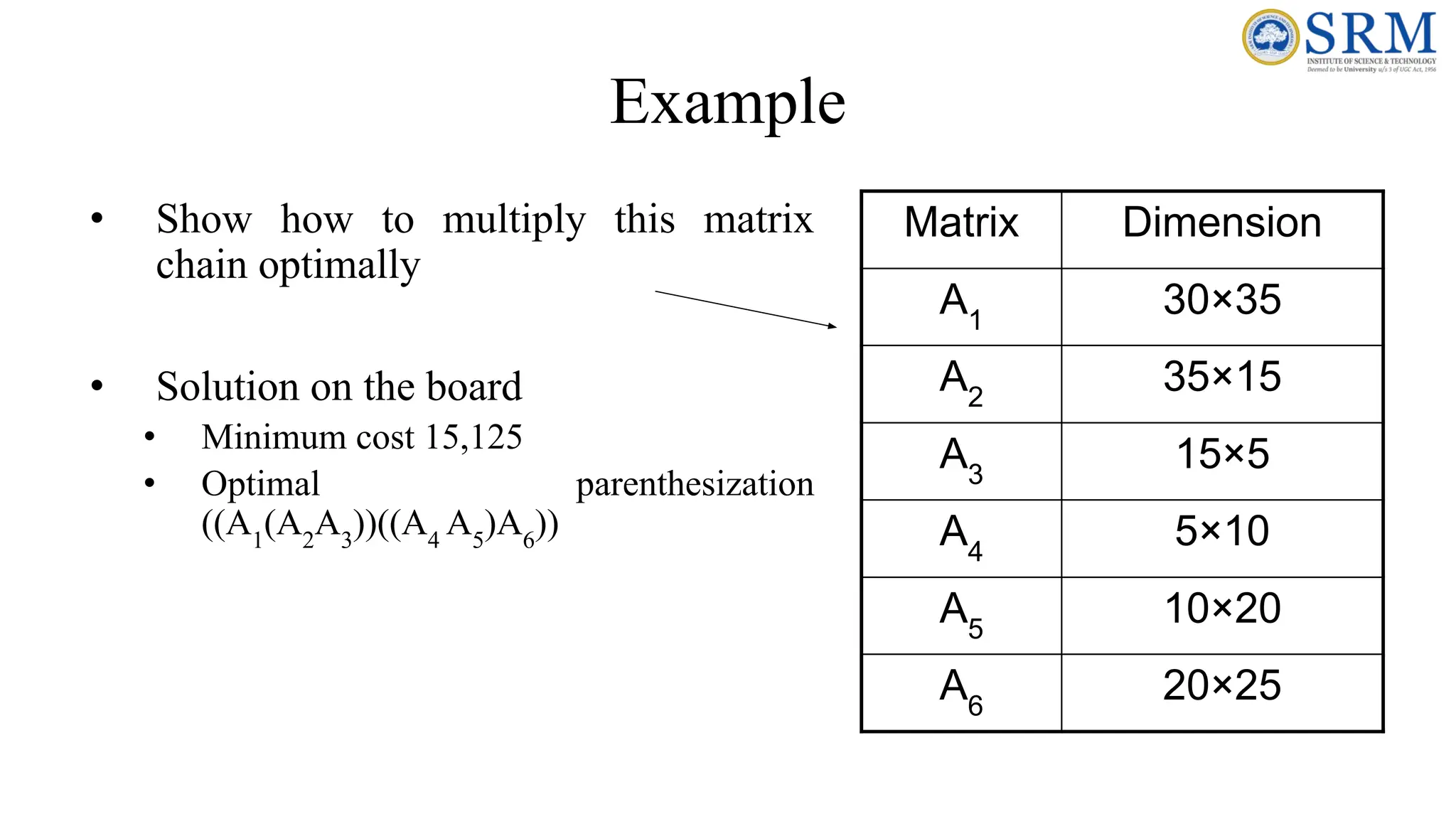

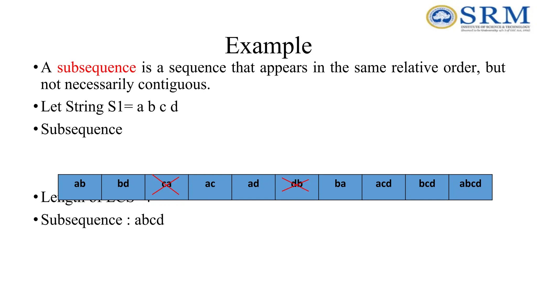


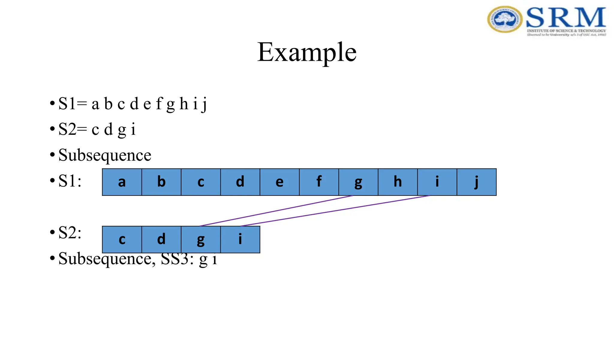
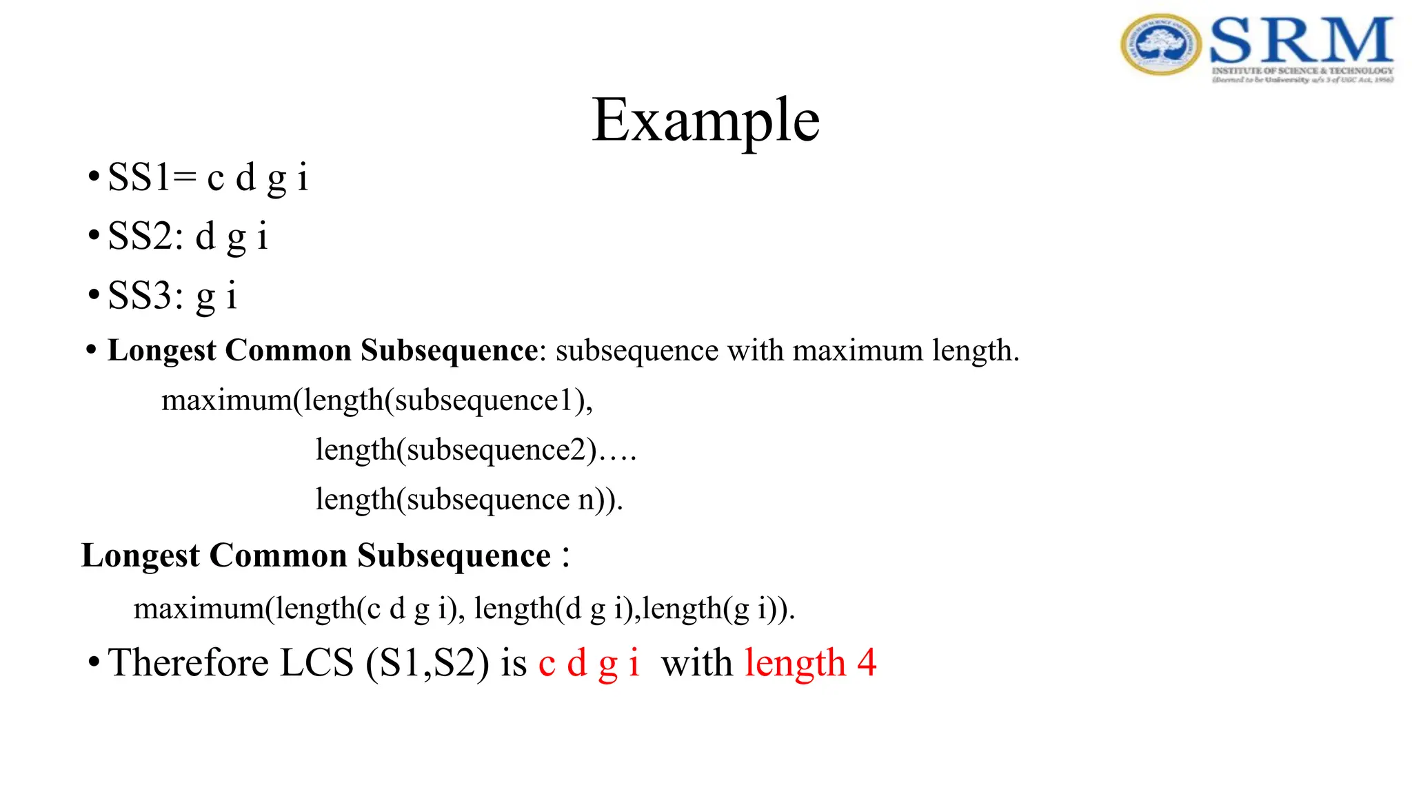
![Motivation Brute Force Approach-Check every subsequence of x[1 . . m] to see if it is also a subsequence of y[1 . . n]. Analysis • 2m subsequences of x (each bit-vector of length m determines a distinct subsequence of x). • Hence, the runtime would be exponential ! Example: Consider S1 = ACCGGTCGAGTGCGCGGAAGCCGGCCGAA….. S2 = GTCGTTCGGAATGCCGTTGCTCTGTAAA…. Towards a better algorithm: a Dynamic Prpgramming strategy • Key: optimal substructure and overlapping sub-problems • First we’ll find the length of LCS. Later we’ll modify the algorithm to find LCS itself.](https://image.slidesharecdn.com/unit3-250731202919-6e165522/75/Unit-4-of-design-and-analysis-of-algorithms-162-2048.jpg)
![LCS Problem Formulation using DP Algorithm • Key: find out the correct order to solve the sub-problems • Total number of sub-problems: m * n c[i, j] = c[i–1, j–1] + 1 if x[i] = y[j], max{c[i–1, j], c[i, j–1]} otherwise. C(i, j) 0 m 0 n i j](https://image.slidesharecdn.com/unit3-250731202919-6e165522/75/Unit-4-of-design-and-analysis-of-algorithms-163-2048.jpg)
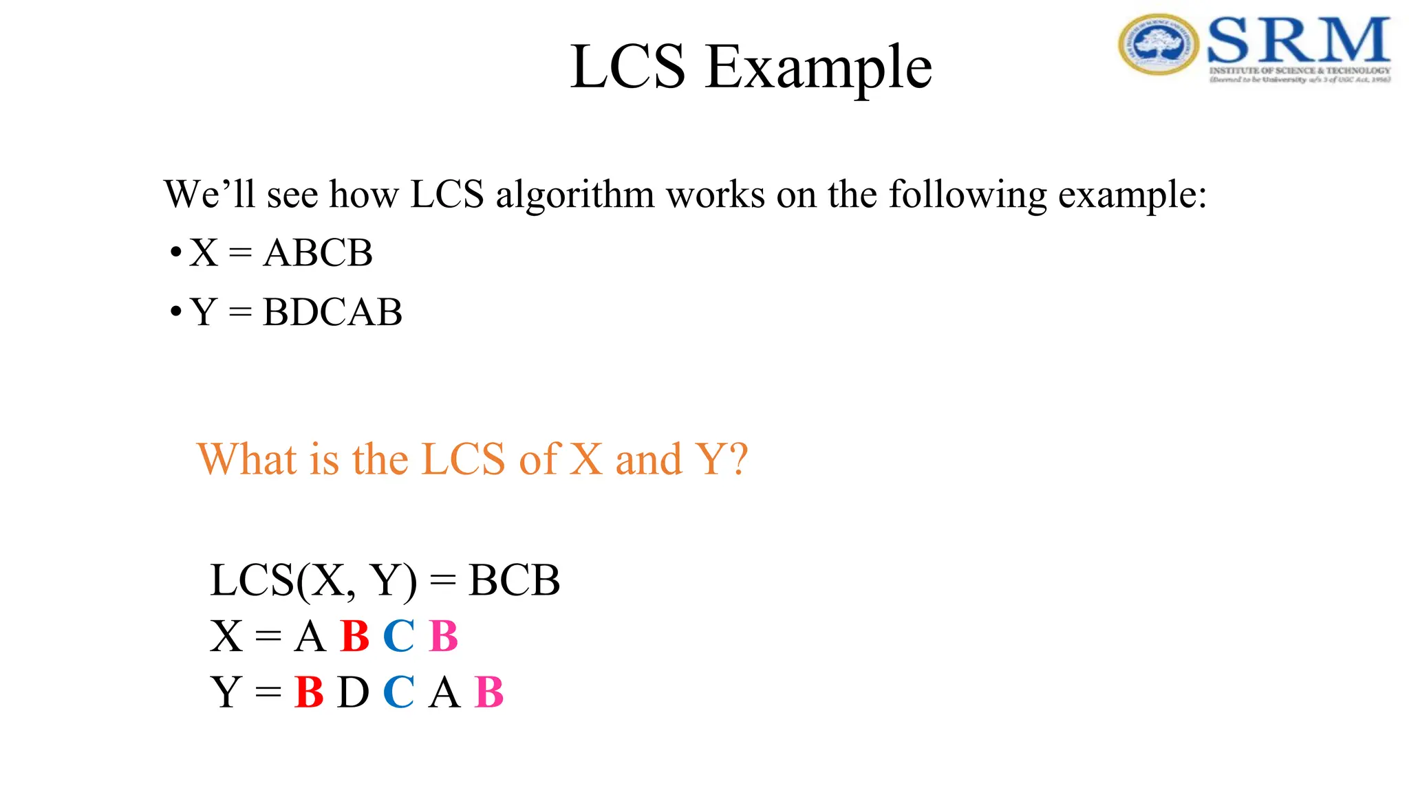
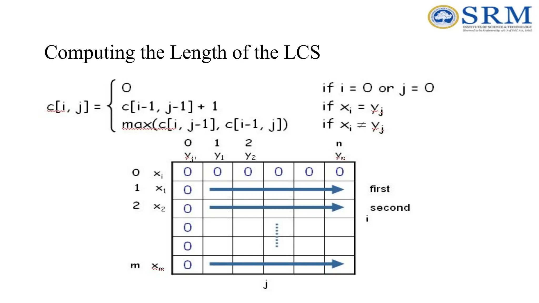
![LCS Example (0) j 0 1 2 3 4 5 0 1 2 3 4 i X[i] A B C B Y[j] B B A C D X = ABCB; m = |X| = 4 Y = BDCAB; n = |Y| = 5 Allocate array c[5,6] ABCB BDCAB](https://image.slidesharecdn.com/unit3-250731202919-6e165522/75/Unit-4-of-design-and-analysis-of-algorithms-166-2048.jpg)
![LCS Example (1) j 0 1 2 3 4 5 0 1 2 3 4 i A B C B B B A C D 0 0 0 0 0 0 0 0 0 0 for i = 1 to m c[i,0] = 0 for j = 1 to n c[0,j] = 0 ABCB BDCAB X[i] Y[j]](https://image.slidesharecdn.com/unit3-250731202919-6e165522/75/Unit-4-of-design-and-analysis-of-algorithms-167-2048.jpg)
![LCS Example (2) j 0 1 2 3 4 5 0 1 2 3 4 i A B C B B B A C D 0 0 0 0 0 0 0 0 0 0 if ( Xi == Yj ) c[i,j] = c[i-1,j-1] + 1 else c[i,j] = max( c[i-1,j], c[i,j-1] ) 0 ABCB BDCAB X[i] Y[j]](https://image.slidesharecdn.com/unit3-250731202919-6e165522/75/Unit-4-of-design-and-analysis-of-algorithms-168-2048.jpg)
![LCS Example (3) j 0 1 2 3 4 5 0 1 2 3 4 i A B C B B B A C D 0 0 0 0 0 0 0 0 0 0 if ( Xi == Yj ) c[i,j] = c[i-1,j-1] + 1 else c[i,j] = max( c[i-1,j], c[i,j-1] ) 0 0 0 ABCB BDCAB X[i] Y[j]](https://image.slidesharecdn.com/unit3-250731202919-6e165522/75/Unit-4-of-design-and-analysis-of-algorithms-169-2048.jpg)
![LCS Example (4) j 0 1 2 3 4 5 0 1 2 3 4 i A B C B B B A C D 0 0 0 0 0 0 0 0 0 0 if ( Xi == Yj ) c[i,j] = c[i-1,j-1] + 1 else c[i,j] = max( c[i-1,j], c[i,j-1] ) 0 0 0 1 ABCB BDCAB X[i] Y[j]](https://image.slidesharecdn.com/unit3-250731202919-6e165522/75/Unit-4-of-design-and-analysis-of-algorithms-170-2048.jpg)
![LCS Example (5) j 0 1 2 3 4 5 0 1 2 3 4 i A B C B B B A C D 0 0 0 0 0 0 0 0 0 0 if ( Xi == Yj ) c[i,j] = c[i-1,j-1] + 1 else c[i,j] = max( c[i-1,j], c[i,j-1] ) 0 0 0 1 1 ABCB BDCAB X[i] Y[j]](https://image.slidesharecdn.com/unit3-250731202919-6e165522/75/Unit-4-of-design-and-analysis-of-algorithms-171-2048.jpg)
![LCS Example (6) j 0 1 2 3 4 5 0 1 2 3 4 i A B C B B B A C D 0 0 0 0 0 0 0 0 0 0 if ( Xi == Yj ) c[i,j] = c[i-1,j-1] + 1 else c[i,j] = max( c[i-1,j], c[i,j-1] ) 0 0 1 0 1 1 ABCB BDCAB X[i] Y[j]](https://image.slidesharecdn.com/unit3-250731202919-6e165522/75/Unit-4-of-design-and-analysis-of-algorithms-172-2048.jpg)
![LCS Example (7) j 0 1 2 3 4 5 0 1 2 3 4 i A B C B B B A C D 0 0 0 0 0 0 0 0 0 0 if ( Xi == Yj ) c[i,j] = c[i-1,j-1] + 1 else c[i,j] = max( c[i-1,j], c[i,j-1] ) 1 0 0 0 1 1 1 1 1 ABCB BDCAB X[i] Y[j]](https://image.slidesharecdn.com/unit3-250731202919-6e165522/75/Unit-4-of-design-and-analysis-of-algorithms-173-2048.jpg)
![LCS Example (8) j 0 1 2 3 4 5 0 1 2 3 4 i A B C B B B A C D 0 0 0 0 0 0 0 0 0 0 if ( Xi == Yj ) c[i,j] = c[i-1,j-1] + 1 else c[i,j] = max( c[i-1,j], c[i,j-1] ) 1 0 0 0 1 1 1 1 1 2 ABCB BDCAB X[i] Y[j]](https://image.slidesharecdn.com/unit3-250731202919-6e165522/75/Unit-4-of-design-and-analysis-of-algorithms-174-2048.jpg)
![LCS Example (9) j 0 1 2 3 4 5 0 1 2 3 4 i A B C B B B A C D 0 0 0 0 0 0 0 0 0 0 if ( Xi == Yj ) c[i,j] = c[i-1,j-1] + 1 else c[i,j] = max( c[i-1,j], c[i,j-1] ) 1 0 0 0 1 2 1 1 1 1 1 1 ABCB BDCAB X[i] Y[j]](https://image.slidesharecdn.com/unit3-250731202919-6e165522/75/Unit-4-of-design-and-analysis-of-algorithms-175-2048.jpg)
![LCS Example (10) j 0 1 2 3 4 5 0 1 2 3 4 i A B C B B B A C D 0 0 0 0 0 0 0 0 0 0 if ( Xi == Yj ) c[i,j] = c[i-1,j-1] + 1 else c[i,j] = max( c[i-1,j], c[i,j-1] ) 1 0 0 0 1 1 2 1 1 1 1 1 2 ABCB BDCAB X[i] Y[j]](https://image.slidesharecdn.com/unit3-250731202919-6e165522/75/Unit-4-of-design-and-analysis-of-algorithms-176-2048.jpg)
![LCS Example (11) j 0 1 2 3 4 5 0 1 2 3 4 i A B C B B B A C D 0 0 0 0 0 0 0 0 0 0 if ( Xi == Yj ) c[i,j] = c[i-1,j-1] + 1 else c[i,j] = max( c[i-1,j], c[i,j-1] ) 1 0 0 0 1 1 2 1 1 1 1 2 1 2 2 ABCB BDCAB X[i] Y[j]](https://image.slidesharecdn.com/unit3-250731202919-6e165522/75/Unit-4-of-design-and-analysis-of-algorithms-177-2048.jpg)
![LCS Example (12) j 0 1 2 3 4 5 0 1 2 3 4 i A B C B B B A C D 0 0 0 0 0 0 0 0 0 0 if ( Xi == Yj ) c[i,j] = c[i-1,j-1] + 1 else c[i,j] = max( c[i-1,j], c[i,j-1] ) 1 0 0 0 1 1 2 1 1 1 1 2 1 2 2 1 ABCB BDCAB X[i] Y[j]](https://image.slidesharecdn.com/unit3-250731202919-6e165522/75/Unit-4-of-design-and-analysis-of-algorithms-178-2048.jpg)
![LCS Example (13) j 0 1 2 3 4 5 0 1 2 3 4 i A B C B B B A C D 0 0 0 0 0 0 0 0 0 0 if ( Xi == Yj ) c[i,j] = c[i-1,j-1] + 1 else c[i,j] = max( c[i-1,j], c[i,j-1] ) 1 0 0 0 1 1 2 1 1 1 1 2 1 2 2 1 1 2 2 ABCB BDCAB X[i] Y[j]](https://image.slidesharecdn.com/unit3-250731202919-6e165522/75/Unit-4-of-design-and-analysis-of-algorithms-179-2048.jpg)
![LCS Example (14) j 0 1 2 3 4 5 0 1 2 3 4 i A B C B B B A C D 0 0 0 0 0 0 0 0 0 0 if ( Xi == Yj ) c[i,j] = c[i-1,j-1] + 1 else c[i,j] = max( c[i-1,j], c[i,j-1] ) 1 0 0 0 1 1 2 1 1 1 1 2 1 2 2 1 1 2 2 3 ABCB BDCAB X[i] Y[j]](https://image.slidesharecdn.com/unit3-250731202919-6e165522/75/Unit-4-of-design-and-analysis-of-algorithms-180-2048.jpg)
![Finding LCS j 0 1 2 3 4 5 0 1 2 3 4 i A B C B B A C D 0 0 0 0 0 0 0 0 0 0 1 0 0 0 1 1 2 1 1 1 1 2 1 2 2 1 1 2 2 3 B X[i] Y[j] Time for trace back: O(m+n).](https://image.slidesharecdn.com/unit3-250731202919-6e165522/75/Unit-4-of-design-and-analysis-of-algorithms-181-2048.jpg)
![Finding LCS (2)(Bottom Up approach) j 0 1 2 3 4 5 0 1 2 3 4 i A B C B B A C D 0 0 0 0 0 0 0 0 0 0 1 0 0 0 1 1 2 1 1 1 1 2 1 2 2 1 1 2 2 3 B B C B LCS: BCB X[i] Y[j]](https://image.slidesharecdn.com/unit3-250731202919-6e165522/75/Unit-4-of-design-and-analysis-of-algorithms-182-2048.jpg)
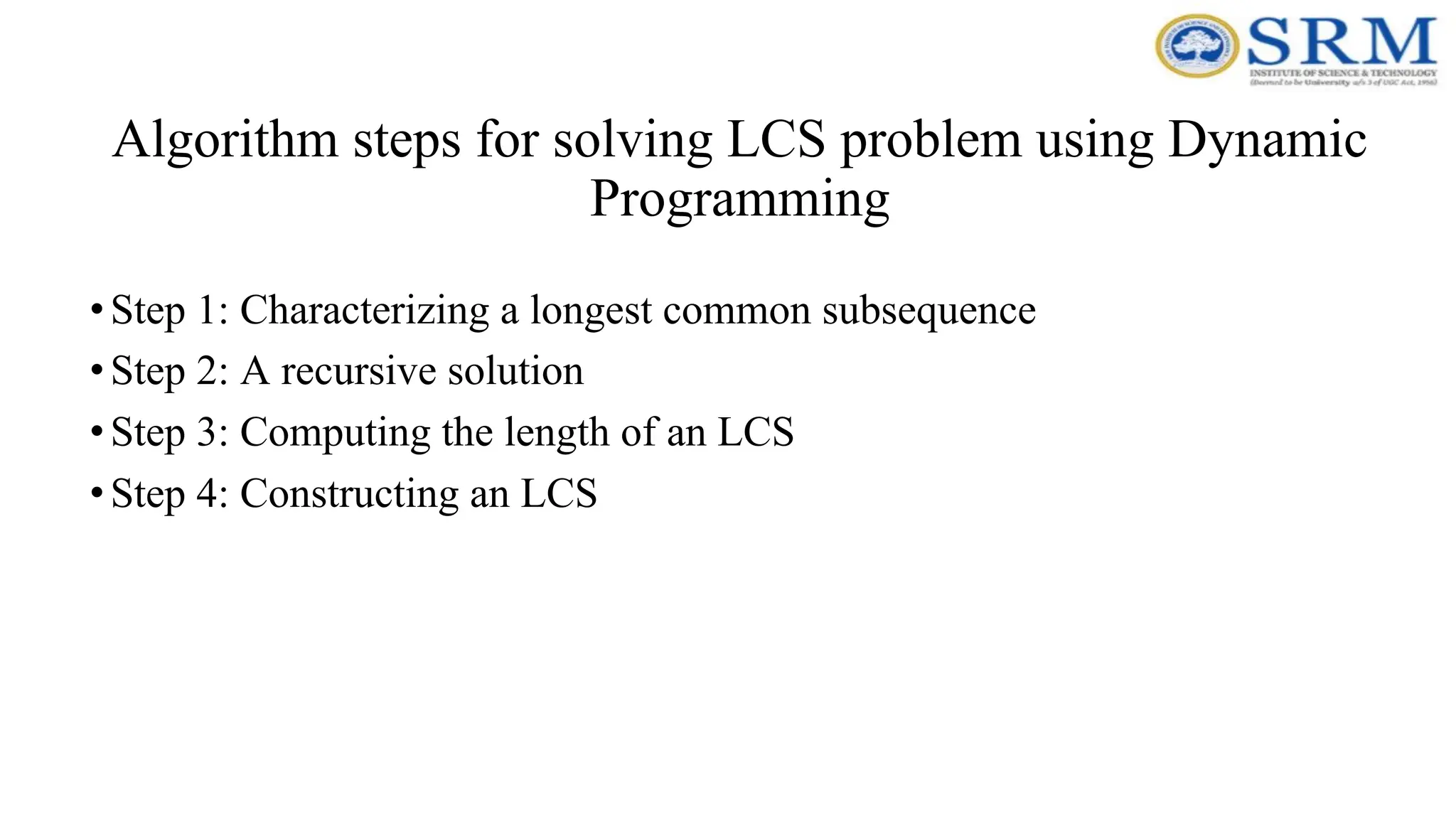
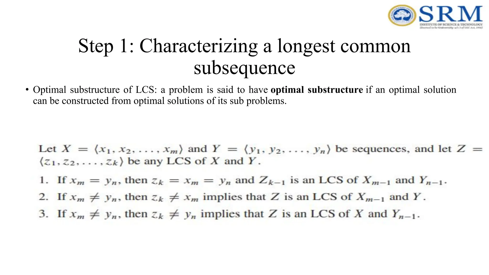
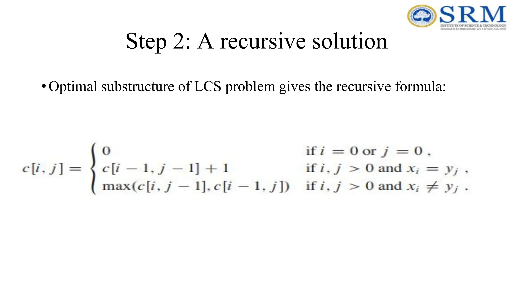

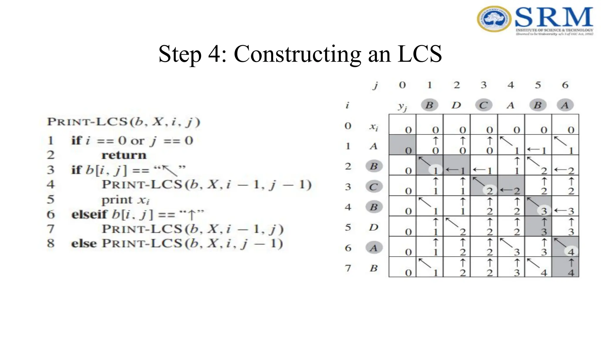
![Time Complexity Analysis of LCS Algorithm •LCS algorithm calculates the values of each entry of the array c[m,n] •So what is the running time? O(m*n) since each c[i,j] is calculated in constant time, and there are m*n elements in the array Asymptotic Analysis: Worst case time complexity: O(n*m) Average case time complexity: O(n*m) Best case time complexity: O(n*m) Space complexity: O(n*m)](https://image.slidesharecdn.com/unit3-250731202919-6e165522/75/Unit-4-of-design-and-analysis-of-algorithms-188-2048.jpg)

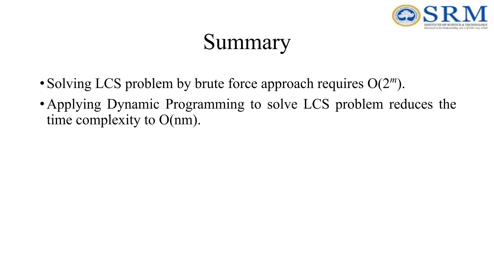
![Review Questions 1. What is the time complexity of the brute force algorithm used to find the longest common subsequence? 2. What is the time complexity of the dynamic programming algorithm used to find the longest common subsequence? 3. If X[i]==Y[i] what is the value stored in c[i,j]? 4. If X[i]!=Y[i] what is the value stored in c[i,j]? 5. What is the value stored in zeroth row and zeroth column of the LCS table?](https://image.slidesharecdn.com/unit3-250731202919-6e165522/75/Unit-4-of-design-and-analysis-of-algorithms-191-2048.jpg)

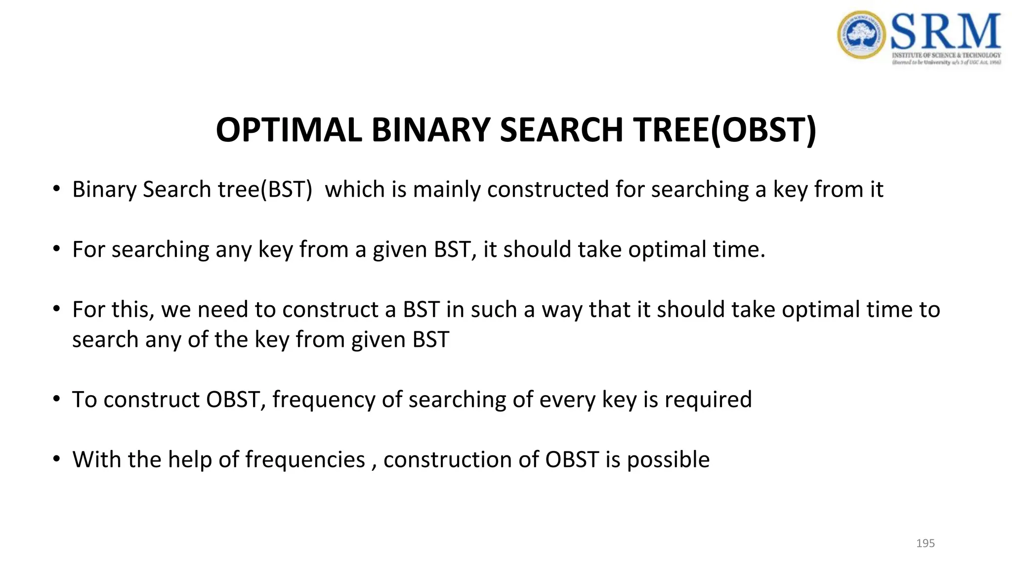
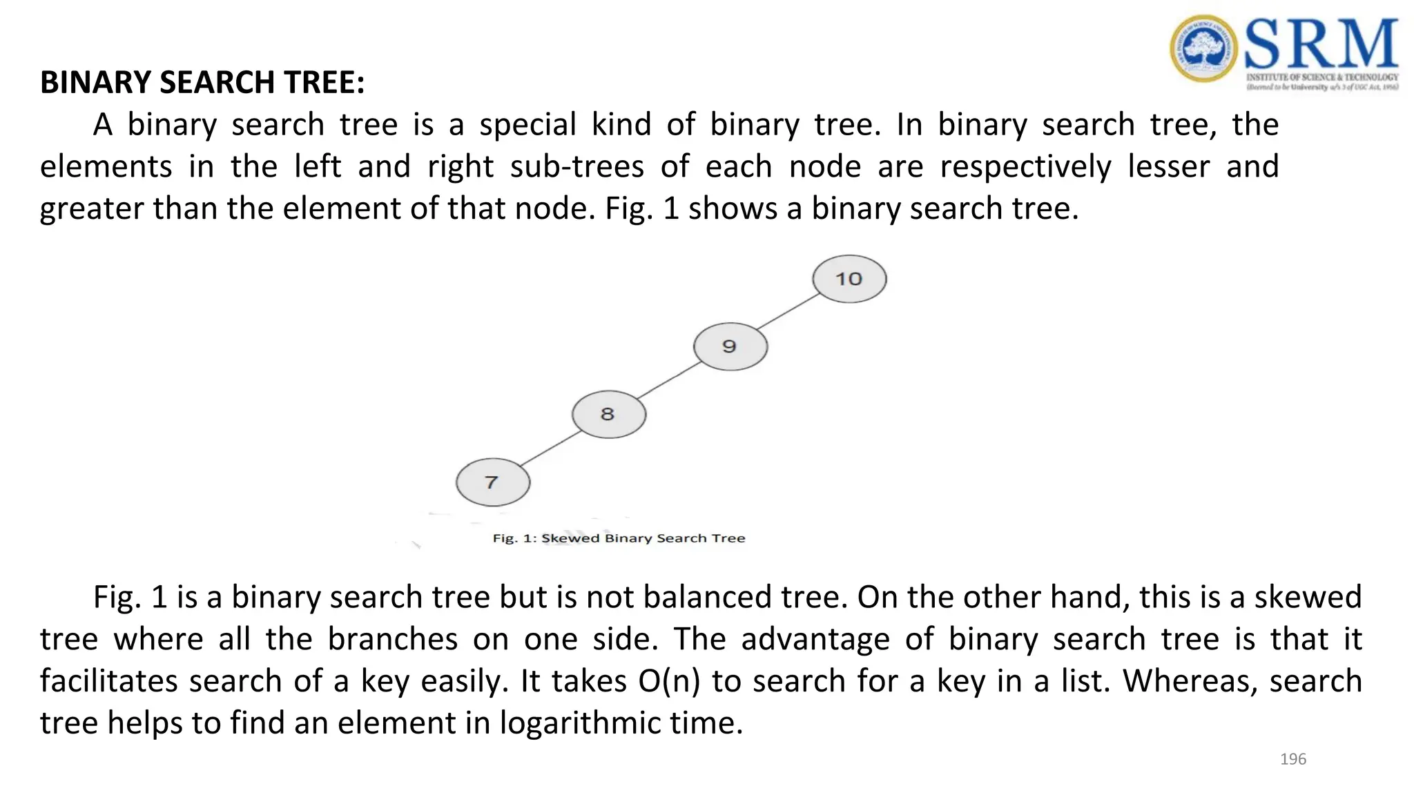
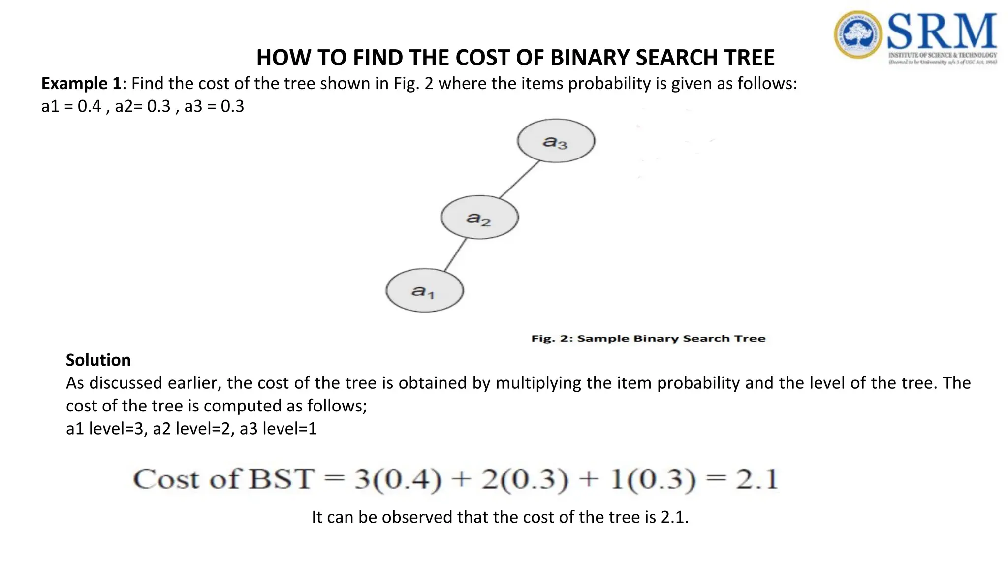
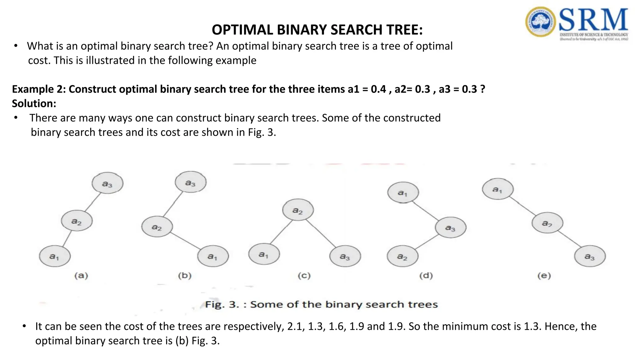
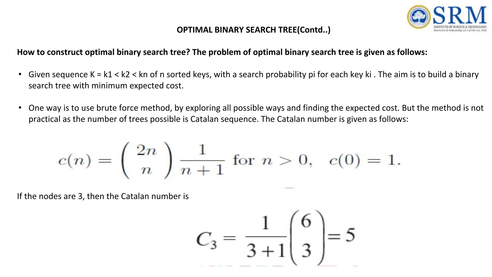
![Hence, five search trees are possible. In general, different BSTs are possible with n nodes. Hence, alternative way is to explore dynamic programming approach. Dynamic programming Approach: • The idea is to One of the keys in a1, …,an , say ak, where 1 ≤ k ≤ n, must be the root. Then , as per binary search rule, Left sub tree of ak contains a1,...,ak1 and right subtree of ak contains ak+1, ...,an. • So, the idea is to examine all candidate roots ak , for 1 ≤ k ≤ n and determining all optimal BSTs containing a1,...,ak1 and containing ak+1,...,an The informal algorithm for constructing optimal BST based on [1,3] is given as follows: OPTIMAL BINARY SEARCH TREE(Contd..)](https://image.slidesharecdn.com/unit3-250731202919-6e165522/75/Unit-4-of-design-and-analysis-of-algorithms-201-2048.jpg)
![The idea is to create a table as shown in below [2] Table 2: Constructed Table for building Optimal BST OPTIMAL BINARY SEARCH TREE WITH DYNAMIC PROGRAMMING](https://image.slidesharecdn.com/unit3-250731202919-6e165522/75/Unit-4-of-design-and-analysis-of-algorithms-202-2048.jpg)
![The idea is to create a table as shown in below [2] Table 2: Constructed Table for building Optimal BST OPTIMAL BINARY SEARCH TREE(Contd..)](https://image.slidesharecdn.com/unit3-250731202919-6e165522/75/Unit-4-of-design-and-analysis-of-algorithms-203-2048.jpg)
![• The aim of the dynamic programming approach is to fill this table for constructing optimal BST. • What should be entry of this table? For example, to compute C[2,3] of two items, say key 2 and key 3, two possible trees are constructed as shown below in Fig. 4 and filling the table with minimum cost. Fig. 4: Two possible ways of BST for key 2 and key 3. OPTIMAL BINARY SEARCH TREE(Contd..)](https://image.slidesharecdn.com/unit3-250731202919-6e165522/75/Unit-4-of-design-and-analysis-of-algorithms-204-2048.jpg)
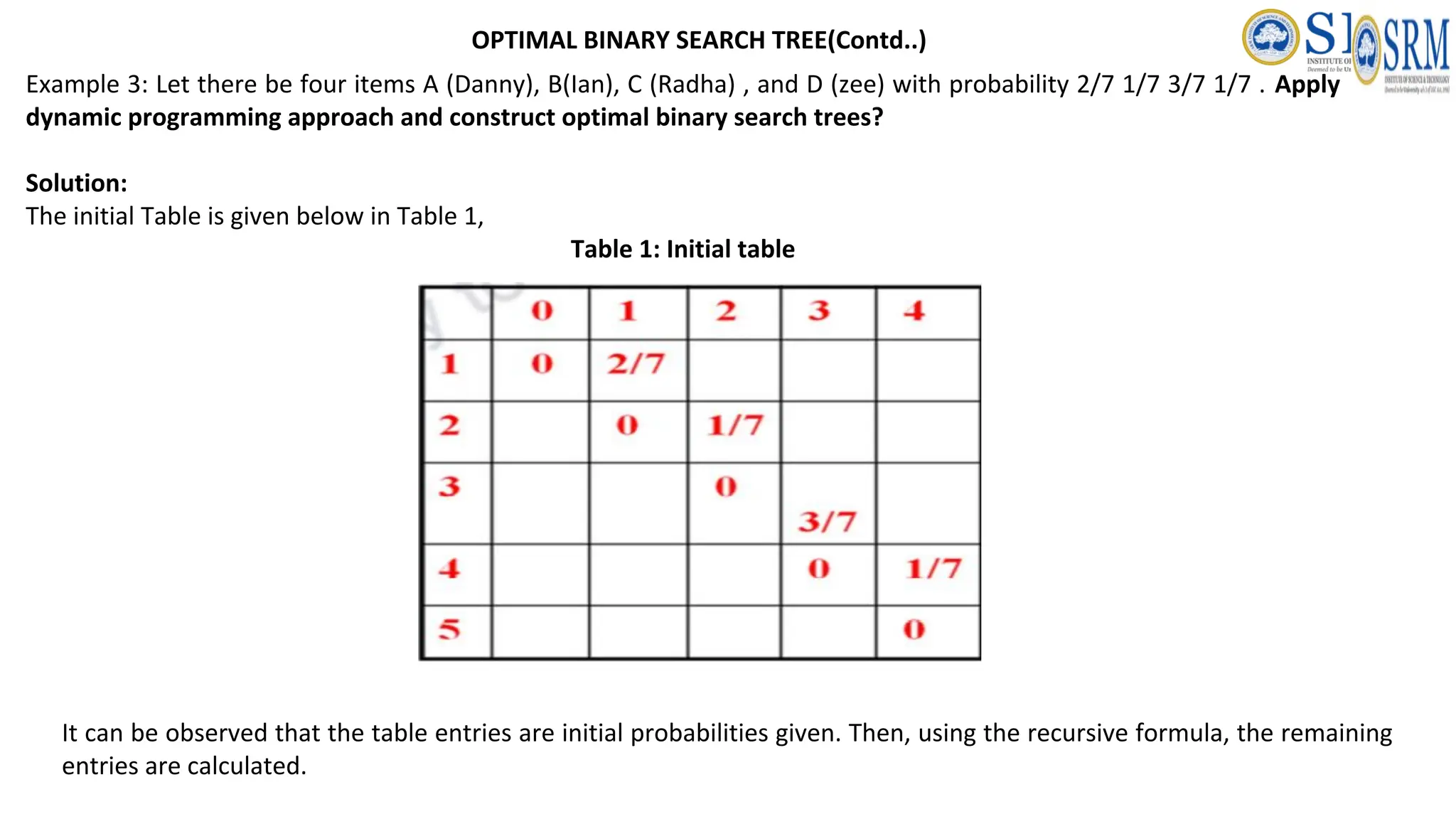
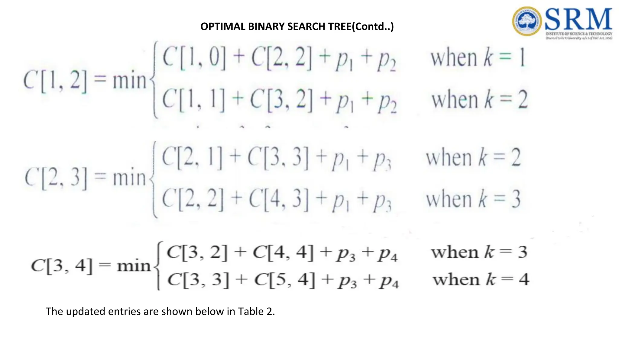
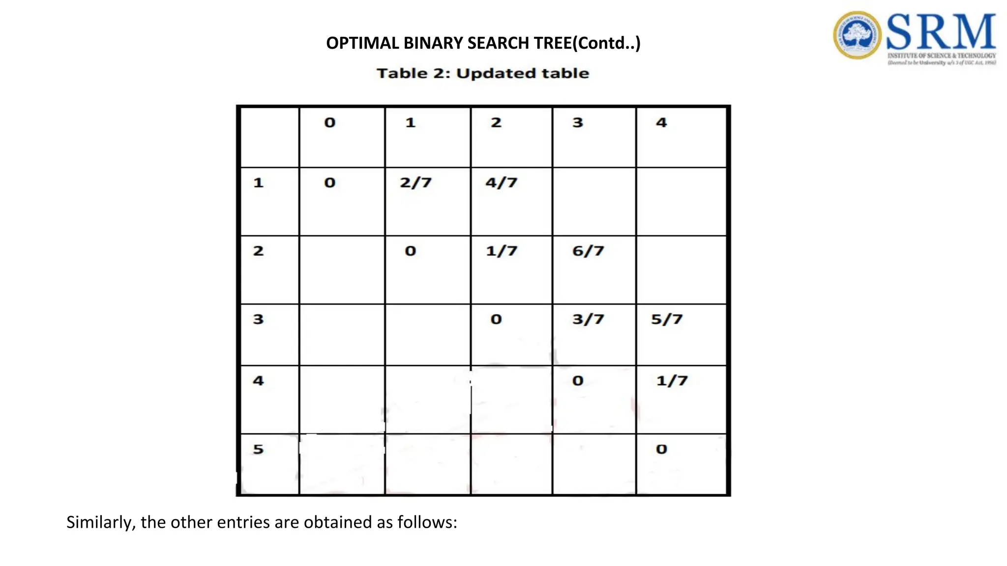
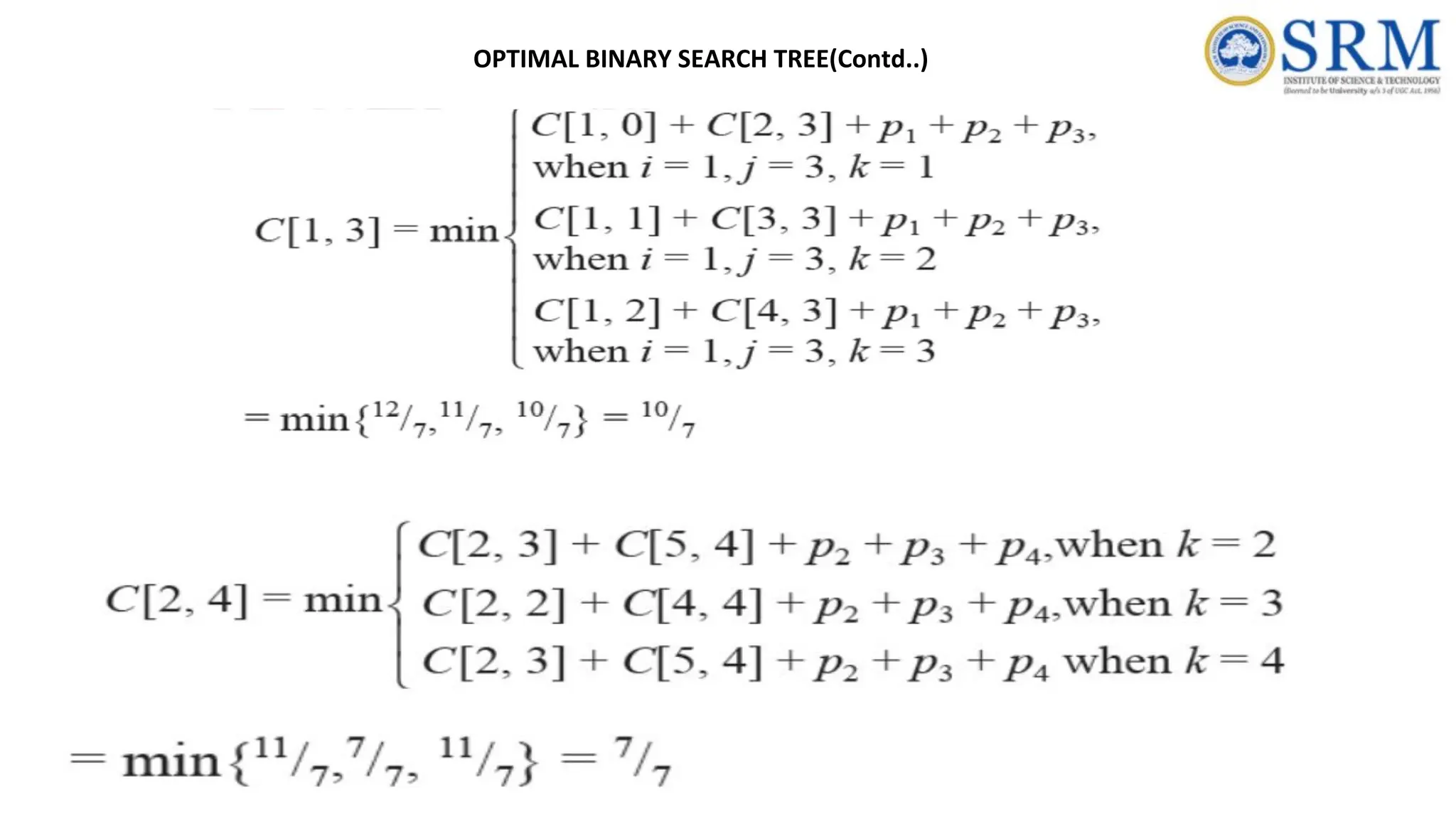
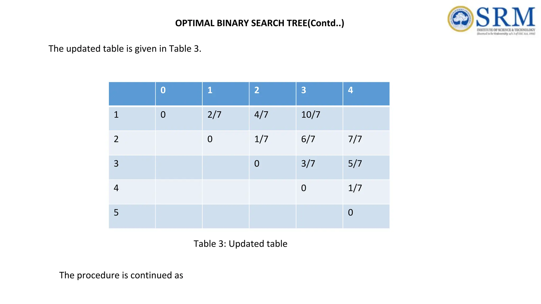

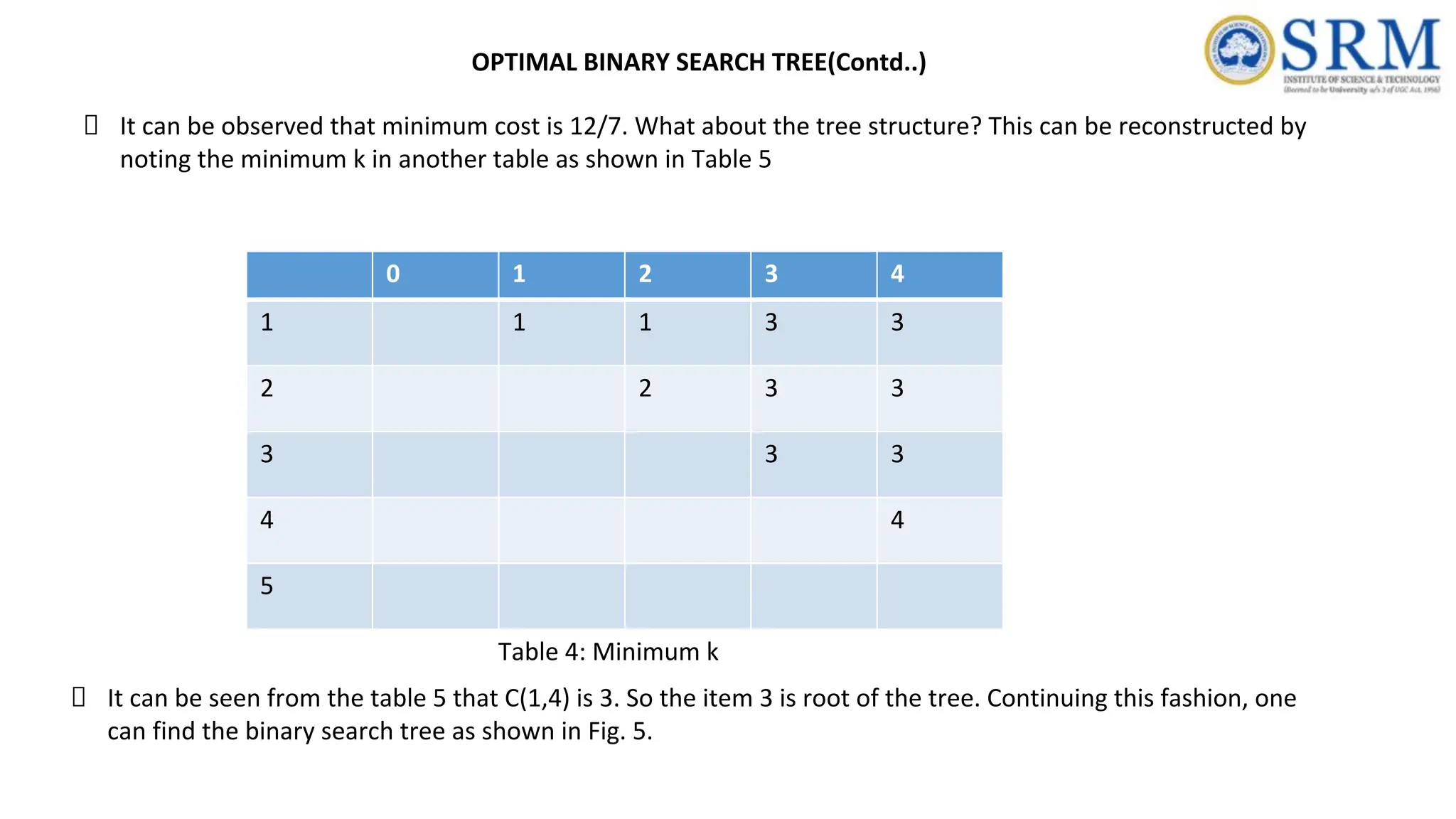
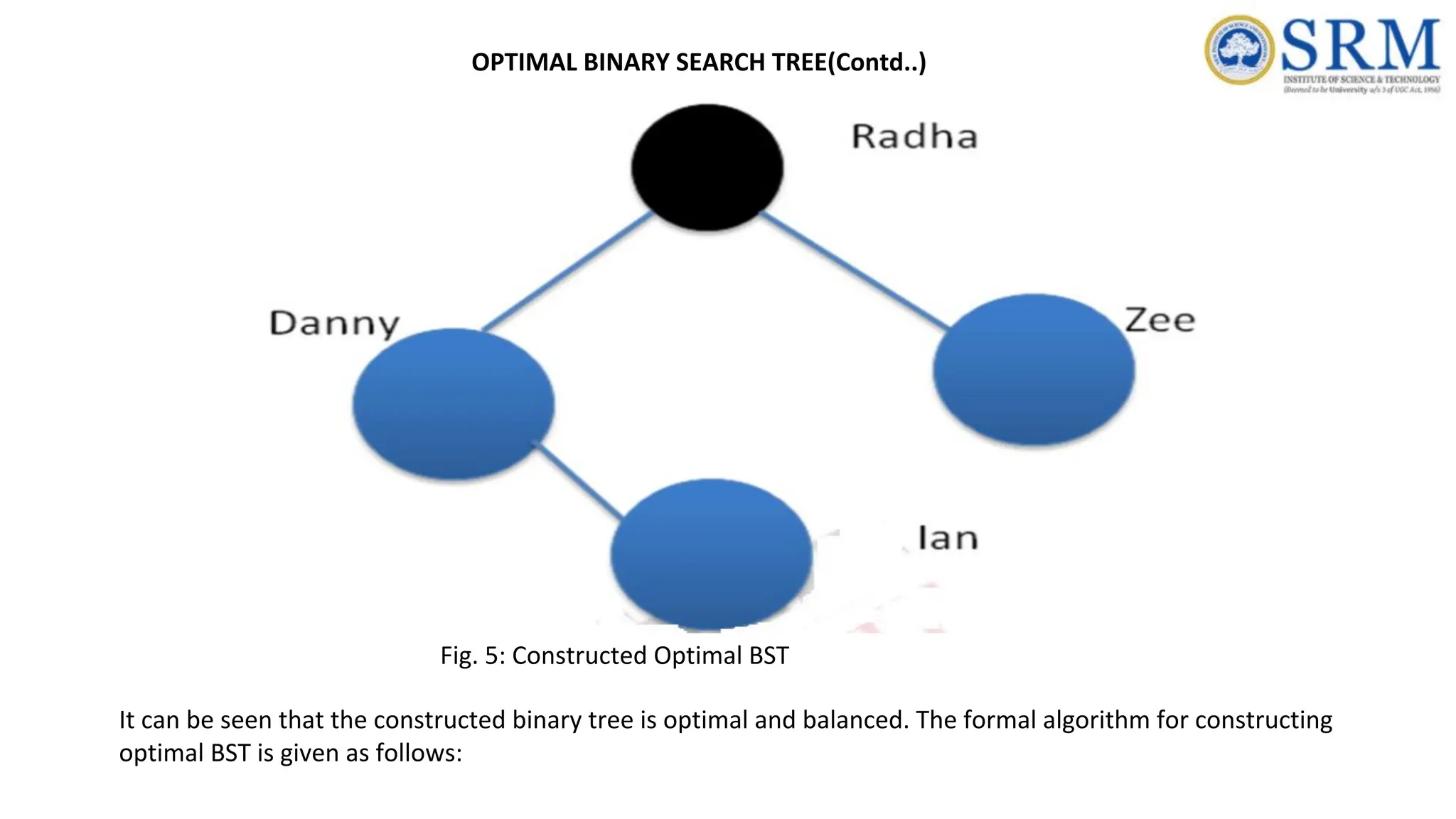
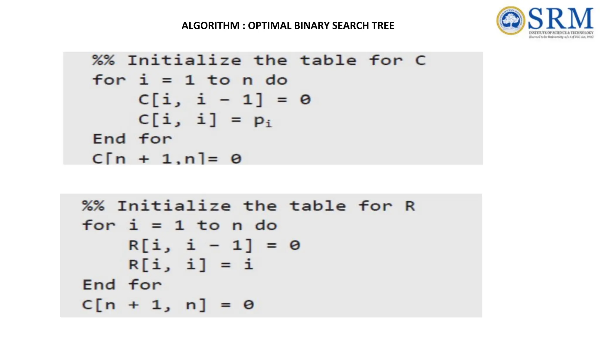
![Complexity Analysis : The time efficiency is Θ (n 3 ) but can be reduced to Θ(n 2 ) by taking advantage of monotonic property of the entries. The monotonic property is that the entry R[i,j] is always in the range between R[i,j-1] and R[i+1,j]. The space complexity is Θ(n 2 ) as the algorithm is reduced to filling the table. ALGORITHM : OPTIMAL BINARY SEARCH TREE](https://image.slidesharecdn.com/unit3-250731202919-6e165522/75/Unit-4-of-design-and-analysis-of-algorithms-214-2048.jpg)