UAV Path Planning using Genetic Algorithm with Parallel Implementation

UAV Path Planning using Genetic Algorithm with Parallel Implementation

• 1.
  International Journal ofComputational Science and Information Technology (IJCSITY) Vol. 10, No. 2, May 2022 DOI : 10.5121/ijcsity.2022.10201 1 UAV PATH PLANNING USING GENETIC ALGORITHMWITH PARALLEL IMPLEMENTATION Mohammad AlRaslan and Ahmad Hilal AlKurdi Faculty of Informatics Engineering, Idleb University, Idleb, Syria ABSTRACT The objective of path planning algorithms is to find the optimal path from a source position to a target position. This paper proposes a real-time path planner for UAVs based on the genetic algorithm. The proposed approach does not identify any specific points outside or between obstacles to solve the problems of the invisible path. In addition, this approach uses no additional steps in the genetic algorithm to handle the problems resulting from generating points inside the obstacles, or the intersection between path segments with obstacles. For these reasons, this paper introduces a simple evaluation method that takes into account the intersections between the path segments and obstacles to find a collision-free and near to optimal path. This evaluation method take into account overlapped and intersected obstacles. The sequential implementation for all of the genetic algorithm steps is detailed. This paper explores the Parallel Genetic Algorithms (PGA) models and introduces the parallel implementation of the proposed path planner on multi-core processors using OpenMP. The execution time of the proposed parallel implementation is reduced compared to sequential execution. KEYWORDS Path planning, UAV, Genetic algorithm, Parallel genetic algorithm, OpenMP, Speed up. 1. INTRODUCTION In recent years, Unmanned Aerial Vehicle (UAV) and Unmanned Ground Vehicle (UGV) Path planningalgorithms become important research topics. These algorithms should find an optimal path between start and target positions. There are two main types of path planning algorithms: global path planning (offline path planning) and local path planning (online path planning) [1–3]. Many studies have detailedand classified path planning algorithms into several categories [4, 5]. Genetic Algorithm (GA) is one of the widely used algorithms for path planning [3]. Many studies implemented GA for UAV path planning and tried to give a collision-free path, where all of the path segments don’t intersect with any obstacle on the map. To avoid an obstacle on the map, many studies suggest to identify specific pointsoutside or between obstacles as crossing points. These points are either randomly generated or at specific locations around the obstacle. Randomly generated points may not be outside the obstacle, and points around obstacles may not give a collision-free path, especially if the obstacles are close to each other or intersect with each other. Other researchers used additional steps in GA to solve the problems resulting from generating points inside the obstacles, or the intersection between the path segments withobstacles. In [6], the Escape operator was introduced in GA for the waypoints that are generated inside the sensing area of radar (obstacle). The solution was to move these waypoints to other positions away from the radar sensing area to get a collision-free path. This means repeating random generation of new waypoints, with condition (if point outside all of obstacles, then …), to reach free waypoint outside obstacles. An Escape method is also presented in [7], with Simulated
• 2.
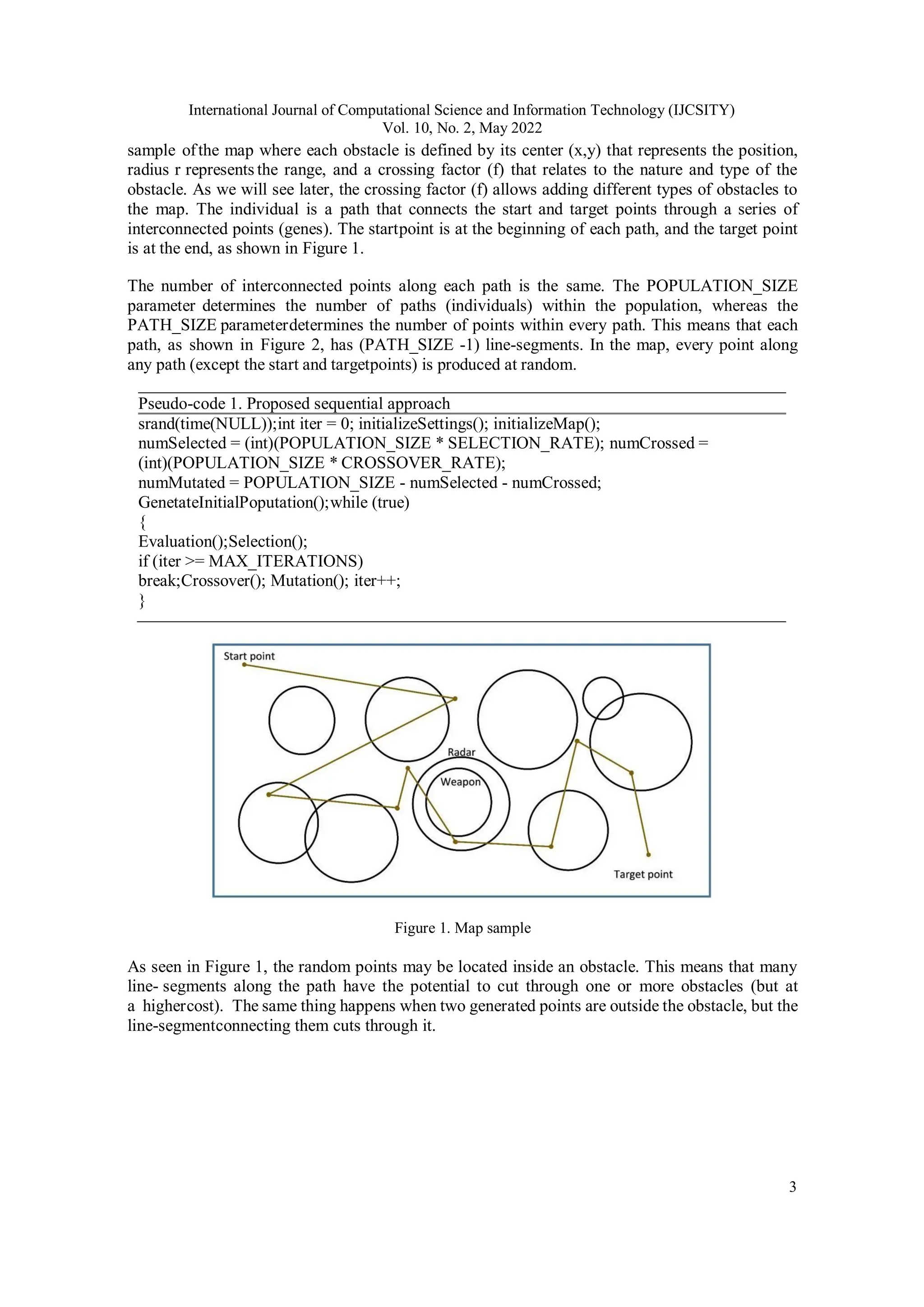
  International Journal ofComputational Science and Information Technology (IJCSITY) Vol. 10, No. 2, May 2022 2 Annealing algorithm. The corner points of a square that covers the threatening radar area (obstacle) are used as crossing points to avoid obstacles. Authors in [8] gave improved GA for path planning. They presented three kinds of path planning schemes: Directly through, Insertion through, and Bypass through. When the path intersects with the threatening region (obstacle), these schemes choose a free path by determining specific pointsfor crossing (mid-point between two threatened zone, or a vertex of threatened zone). The improved GA in [8], has been modified in [9]. Likewise, the authors relied on that the path is feasible when all the guidance points are feasible. An avoiding technique was proposed in [10], by adding eight virtual points as crossing points. These points are placed in the orbit of the radar with a 45° angle. Simulated Annealing algorithm is used in [11], and two methods are introduced to give a good optimal solution that at the same time avoids circular radar threats (2-Opt method and two nodes random swapping method). The 2-Opt method stops at a point where it cannot improve the path because of the radar areas.The resulted path was not optimal in some of the cases when the number of radar threats is high (6-8). Authors in [12] used GA and presented a Forbidden Zone avoidance technique. The Forbidden Zone’s shape is assumed as a square type. This technique relies on covering the Forbidden Zones with the Guard Zones. When the path is invisible, specific points are used (one or two Guard Zones corner points) and added to the path. The researcher mention that this technique works when there is no overlapbetween the Forbidden Zones. Furthermore, most current path planning studies did not stop at just presenting the algorithm model; they also provided a parallel model for this algorithm to achieve real-time path planning. This paper proposes an approach for real-time UAV path planning. This approach deals with all points in search space as a crossable point. We discuss all GA steps and introduce a simple evaluation methodto find a collision-free and near to optimal path. This method takes into account the intersection states between the path segments and the obstacles. In addition, it does not specify any points on the map to solve the problems of the invisible path. The evaluation method deals with intersected or overlapped obstacles. After that, we detail how we achieved parallelism on multi-core systems. We present the Parallel Genetic Algorithms (PGA) and its implementation models and discuss implementation details of this approach on multicore architecture using OpenMP. We compare the sequential time with the parallel time and introduce the speed up. The remainder of this paper is organized as follows: Section 2 introduces GA principles and contains the proposed sequential approach for path planning. Section 3 deals with parallel computing, OpenMP, and parallel genetic algorithm (PGA). Section 4 presents the proposed parallel implementation. Section 5 focuses on simulation and experimental results. Finally, we conclude the paper in Section 6. 2. PROPOSED SEQUENTIAL APPROACH This section introduces all proposed GA steps for path planning. GA is usually started with a populationof individuals (chromosomes). Each individual is made up of a set of genes. The first task in GA is to figure out how to describe the environment, represent individuals, and calculate fitness. Following that,GA begins to develop solutions utilizing the following steps: crossover, mutation, and selection. Pseudo-code 1, describes the GA steps in our code. These steps are repeated until satisfying a condition,which is the number of iterations. 2.1. Environment modelling and chromosome encoding We propose the environment as a 2-D map, with several circular obstacles. These obstacles may represent a radar sensing range, enemy weapon zones, or difficult terrain. Figure 1, shows a
• 3.
  International Journal ofComputational Science and Information Technology (IJCSITY) Vol. 10, No. 2, May 2022 3 sample ofthe map where each obstacle is defined by its center (x,y) that represents the position, radius r represents the range, and a crossing factor (f) that relates to the nature and type of the obstacle. As we will see later, the crossing factor (f) allows adding different types of obstacles to the map. The individual is a path that connects the start and target points through a series of interconnected points (genes). The startpoint is at the beginning of each path, and the target point is at the end, as shown in Figure 1. The number of interconnected points along each path is the same. The POPULATION_SIZE parameter determines the number of paths (individuals) within the population, whereas the PATH_SIZE parameterdetermines the number of points within every path. This means that each path, as shown in Figure 2, has (PATH_SIZE -1) line-segments. In the map, every point along any path (except the start and targetpoints) is produced at random. Pseudo-code 1. Proposed sequential approach srand(time(NULL));int iter = 0; initializeSettings(); initializeMap(); numSelected = (int)(POPULATION_SIZE * SELECTION_RATE); numCrossed = (int)(POPULATION_SIZE * CROSSOVER_RATE); numMutated = POPULATION_SIZE - numSelected - numCrossed; GenetateInitialPoputation();while (true) { Evaluation();Selection(); if (iter >= MAX_ITERATIONS) break;Crossover(); Mutation(); iter++; } Figure 1. Map sample As seen in Figure 1, the random points may be located inside an obstacle. This means that many line- segments along the path have the potential to cut through one or more obstacles (but at a highercost). The same thing happens when two generated points are outside the obstacle, but the line-segmentconnecting them cuts through it.
• 4.
  International Journal ofComputational Science and Information Technology (IJCSITY) Vol. 10, No. 2, May 2022 4 Figure 2. Population and individual representation Table 1 gives the parameters of the genetic algorithm and the map. All of these parameters are initializedat the beginning of the algorithm. Table 1. The parameters of GA and the map parameter significance POPULATION_SIZE the number of individuals (paths) in population PATH_SIZE the number of the points in every path MAX_ITERATIONS the maximum number of repetitions in GA while loop SELECTION_RATE selection rate CROSSOVER_RATE crossover rate MUTATION_RATE mutation rate MaxX the maximum value on the X-axis MaxY the maximum value on the Y-axis source the source point target the target point obstacles[] an array of obstacles 2.2. Generating initial population The first step in GA is to generate the initial population. Paths within the initial population are createdat random. As illustrated in Figure 2, we need to generate (PATH_SIZE-2) random points for each pathbetween start and target points (𝑃1 → 𝑃PATH_SIZE − 2 ). Pseudo-code 2. Generating initial population void GenetateInitialPoputation() { for (int i = 0; i < POPULATION_SIZE; i++) { myPop[i].path[0] = myMap->source; for (int j = 1; j < PATH_SIZE - 1; j++) { myPop[i].path[j] = getRandomPoint(); } myPop[i].path[PATH_SIZE - 1] = myMap->dist; } } Generating a random point is achieved by generating its coordinate (x,y) on the map. These
• 5.
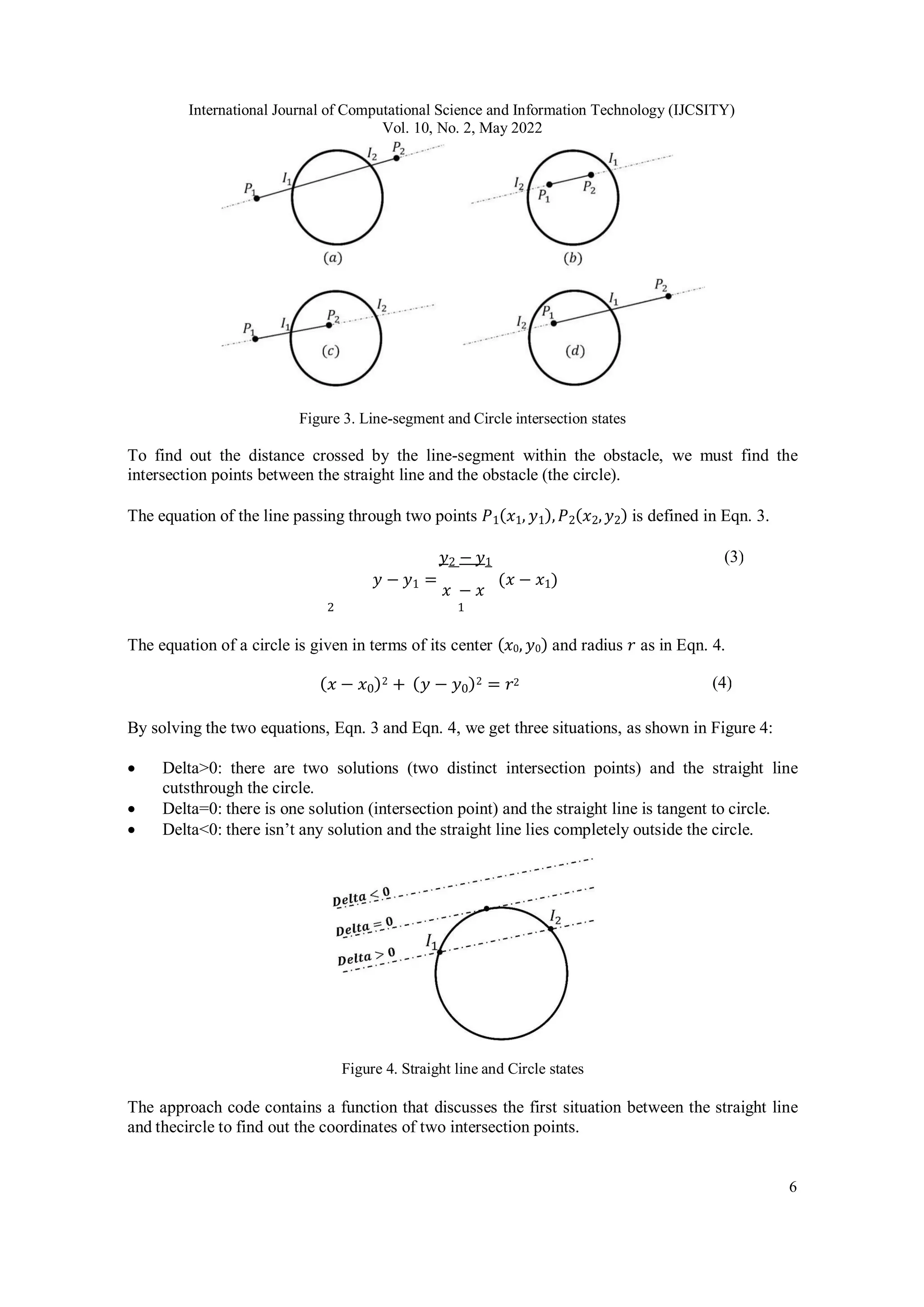
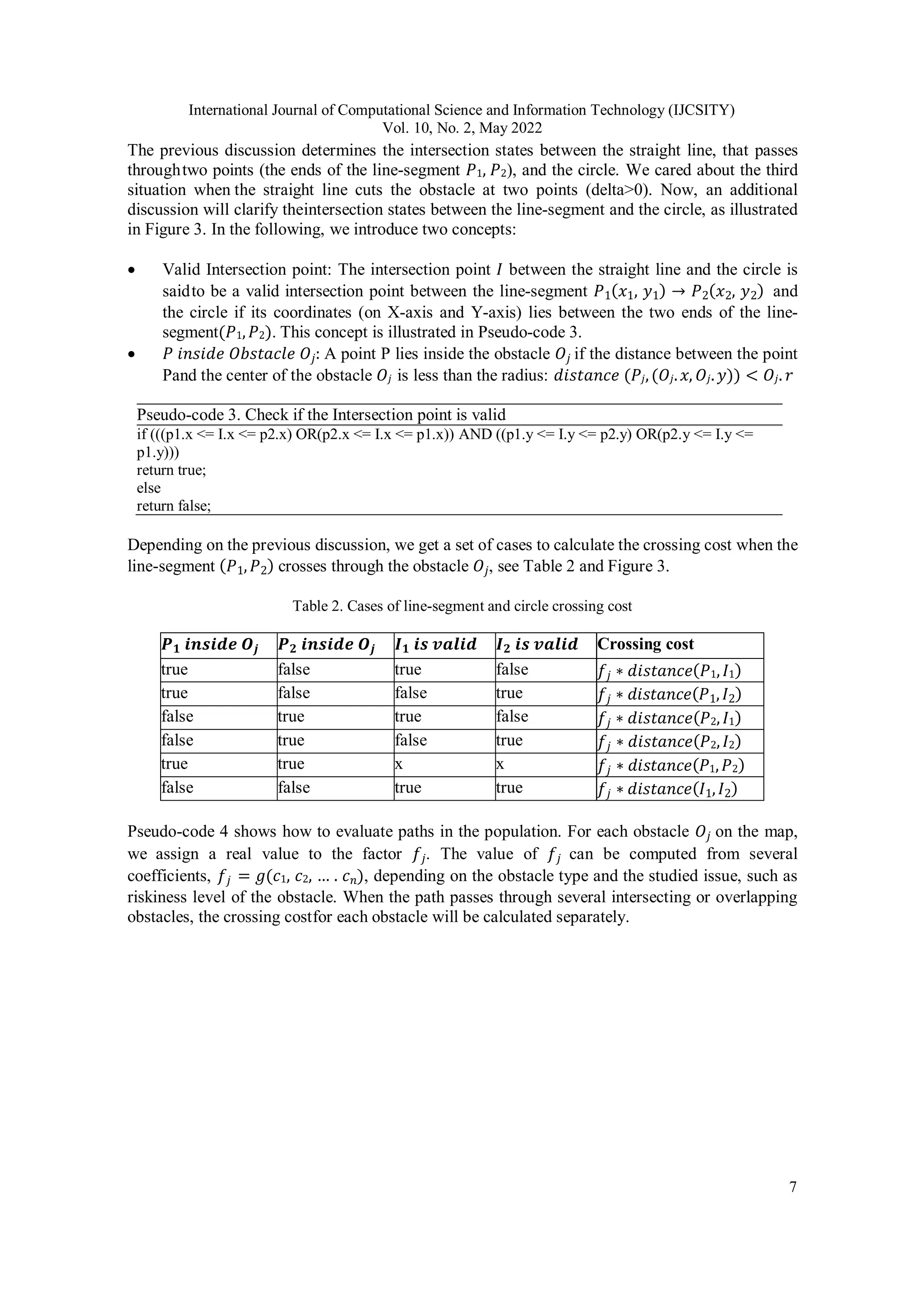
  International Journal ofComputational Science and Information Technology (IJCSITY) Vol. 10, No. 2, May 2022 5 coordinates are specified in the [0, MaxX] and [0,MaxY] ranges on X-axis and Y-axis, respectively. The rand() andsrand() functions in the C++ language can be used to generate random numbers. Pseudo-code 2 includesthe generating initial population step. 2.3. Evaluation As mentioned earlier, path points are generated at random inside the map. This means that some pointscan be placed within the obstacles. In addition, two neighbouring points can be outside the obstacle, while the line-segment connecting them cuts through the obstacle. In this study, and depending on the previous assumptions, the fitness function evaluates the path in two aspects: basic cost and crossing cost, as illustrated in Eqn. 1 and Eqn. 2. 𝑡𝑜𝑡𝑎𝑙 𝑐𝑜𝑠𝑡(𝑓𝑖𝑡𝑛𝑒𝑠𝑠) = 𝑏𝑎𝑠𝑖𝑐 𝑐𝑜𝑠𝑡 + 𝑐𝑟𝑜𝑠𝑠𝑖𝑛𝑔 𝑐𝑜𝑠𝑡 (1) The basic cost is the path’s length. To put it another way, the path's length is the sum of the lengths of the line-segments that make it up. Euclidean distance is used to calculate the distance between two points. The crossing cost is calculated for line-segments within the path that travelled across one or more obstacles. The crossing cost relates to the crossing distance within the obstacle and a factor f. Thisfactor relates to the nature and type of the obstacle, where there is a possibility to add different type ofobstacles (in crossing cost) to the map, and to deal with overlapped or intersected obstacles. 𝑛−1 𝑚−1 𝐹𝑖𝑡𝑛𝑒𝑠𝑠(𝑝𝑎𝑡ℎ𝑘) = ∑ ( 𝐷𝑖𝑠𝑡𝑎𝑛𝑐𝑒(𝑃𝑖, 𝑃𝑖+1) + ∑ 𝑓𝑗 ∗ 𝐶𝑟𝑜𝑠𝑖𝑛𝑔𝐶𝑜𝑠𝑡(𝑃𝑖, 𝑃𝑖+1, 𝑂𝑗)) 𝑖=0 𝑗=0 (2) Where:  n: is the number of line-segments in each path (individual).  m: is the number of obstacles on the map.  𝑓𝑖𝑡𝑛𝑒𝑠𝑠(𝑝𝑎𝑡ℎ𝑘): denotes the total cost (fitness) of the Kth path, which represents the Kth individual in the population.  𝐷𝑖𝑠𝑡𝑎𝑛𝑐𝑒(𝑃𝑖, 𝑃𝑖+1): is the Euclidian distance between the two points 𝑃𝑖, 𝑃𝑖+1 within the path.  𝐶𝑟𝑜𝑠𝑖𝑛𝑔𝐶𝑜𝑠𝑡(𝑃𝑖, 𝑃𝑖+1, 𝑂𝑗): refers to the crossing cost when line-segment (𝑃𝑖, 𝑃𝑖+1) crossed through the obstacle (𝑂𝑗).  𝑓𝑗: is a factor that depends on the type of obstacle 𝑂𝑗 and the issue at hand Figure 3 explains the intersection states between a line-segment and the obstacle that is represented bya circle. Calculating the crossing distance has many cases based on these states. In the first state, Figure3 (a), there are two intersection points 𝐼1, 𝐼2. The crossing cost is the distance from 𝐼1 to 𝐼2 multiplied by the factor f. Based on Eqn. 2, the overall crossing cost for the line- segment (𝑃1,𝑃2) is calculated foreach obstacle 𝑂𝑗.
• 6.
  International Journal ofComputational Science and Information Technology (IJCSITY) Vol. 10, No. 2, May 2022 6 Figure 3. Line-segment and Circle intersection states To find out the distance crossed by the line-segment within the obstacle, we must find the intersection points between the straight line and the obstacle (the circle). The equation of the line passing through two points 𝑃1(𝑥1, 𝑦1),𝑃2(𝑥2,𝑦2) is defined in Eqn. 3. 𝑦2 − 𝑦1 𝑦 − 𝑦1 = 𝑥 − 𝑥 (𝑥 − 𝑥1) 2 1 (3) The equation of a circle is given in terms of its center (𝑥0, 𝑦0) and radius 𝑟 as in Eqn. 4. (𝑥 − 𝑥0)2 + (𝑦 − 𝑦0)2 = 𝑟2 (4) By solving the two equations, Eqn. 3 and Eqn. 4, we get three situations, as shown in Figure 4:  Delta>0: there are two solutions (two distinct intersection points) and the straight line cutsthrough the circle.  Delta=0: there is one solution (intersection point) and the straight line is tangent to circle.  Delta<0: there isn’t any solution and the straight line lies completely outside the circle. Figure 4. Straight line and Circle states The approach code contains a function that discusses the first situation between the straight line and thecircle to find out the coordinates of two intersection points.
• 7.
  International Journal ofComputational Science and Information Technology (IJCSITY) Vol. 10, No. 2, May 2022 7 The previous discussion determines the intersection states between the straight line, that passes throughtwo points (the ends of the line-segment 𝑃1, 𝑃2), and the circle. We cared about the third situation when the straight line cuts the obstacle at two points (delta>0). Now, an additional discussion will clarify theintersection states between the line-segment and the circle, as illustrated in Figure 3. In the following, we introduce two concepts:  Valid Intersection point: The intersection point 𝐼 between the straight line and the circle is saidto be a valid intersection point between the line-segment 𝑃1(𝑥1, 𝑦1) → 𝑃2(𝑥2, 𝑦2) and the circle if its coordinates (on X-axis and Y-axis) lies between the two ends of the line- segment(𝑃1,𝑃2). This concept is illustrated in Pseudo-code 3.  𝑃 𝑖𝑛𝑠𝑖𝑑𝑒 𝑂𝑏𝑠𝑡𝑎𝑐𝑙𝑒 𝑂𝑗: A point P lies inside the obstacle 𝑂𝑗 if the distance between the point Pand the center of the obstacle 𝑂𝑗 is less than the radius: 𝑑𝑖𝑠𝑡𝑎𝑛𝑐𝑒 (𝑃𝑗,(𝑂𝑗.𝑥, 𝑂𝑗.𝑦)) < 𝑂𝑗. 𝑟 Pseudo-code 3. Check if the Intersection point is valid if (((p1.x <= I.x <= p2.x) OR(p2.x <= I.x <= p1.x)) AND ((p1.y <= I.y <= p2.y) OR(p2.y <= I.y <= p1.y))) return true; else return false; Depending on the previous discussion, we get a set of cases to calculate the crossing cost when the line-segment (𝑃1,𝑃2) crosses through the obstacle 𝑂𝑗, see Table 2 and Figure 3. Table 2. Cases of line-segment and circle crossing cost 𝑷𝟏 𝒊𝒏𝒔𝒊𝒅𝒆 𝑶𝒋 𝑷𝟐 𝒊𝒏𝒔𝒊𝒅𝒆 𝑶𝒋 𝑰𝟏 𝒊𝒔 𝒗𝒂𝒍𝒊𝒅 𝑰𝟐 𝒊𝒔 𝒗𝒂𝒍𝒊𝒅 Crossing cost true false true false 𝑓𝑗 ∗ 𝑑𝑖𝑠𝑡𝑎𝑛𝑐𝑒(𝑃1,𝐼1) true false false true 𝑓𝑗 ∗ 𝑑𝑖𝑠𝑡𝑎𝑛𝑐𝑒(𝑃1,𝐼2) false true true false 𝑓𝑗 ∗ 𝑑𝑖𝑠𝑡𝑎𝑛𝑐𝑒(𝑃2,𝐼1) false true false true 𝑓𝑗 ∗ 𝑑𝑖𝑠𝑡𝑎𝑛𝑐𝑒(𝑃2,𝐼2) true true x x 𝑓𝑗 ∗ 𝑑𝑖𝑠𝑡𝑎𝑛𝑐𝑒(𝑃1,𝑃2) false false true true 𝑓𝑗 ∗ 𝑑𝑖𝑠𝑡𝑎𝑛𝑐𝑒(𝐼1,𝐼2) Pseudo-code 4 shows how to evaluate paths in the population. For each obstacle 𝑂𝑗 on the map, we assign a real value to the factor 𝑓𝑗. The value of 𝑓𝑗 can be computed from several coefficients, 𝑓𝑗 = 𝑔(𝑐1, 𝑐2, … . 𝑐𝑛), depending on the obstacle type and the studied issue, such as riskiness level of the obstacle. When the path passes through several intersecting or overlapping obstacles, the crossing costfor each obstacle will be calculated separately.
• 8.
  International Journal ofComputational Science and Information Technology (IJCSITY) Vol. 10, No. 2, May 2022 8 Pseudo-code 4. Evaluation step void Evaluation() { for (int i = 0; i < POPULATION_SIZE; i++) { for (int j = 0; j < PATH_SIZE - 1; j++) { BasicCostOnePath+=EuclideanDistance (myPop[i].path[j], myPop[i].path[j + 1]); CrossingCostOnePath+=CrossingCostInAllObstacles(myPop[i].path[j], myPop[i].path[j + 1]); } TotalCostOnePath = BasicCostOnePath + CrossingCostOnePath;myPop[i].Fitness = TotalCostOnePath; BasicCostOnePath=TotalCostOnePath=CrossingCostOnePath=0; } } 2.4. Selection The selection step's goal is to choose the best individuals for the next generation. In this work, the rankselection method is employed. Firstly, all individuals are sorted in descending order, with the fitness value as the sort key. Then they are selected (saved) to the new population. (SELECTION RATE*POPULATION SIZE) determines the number of selected paths. The sorting algorithm has an impact on GA's execution time. MergeSort, which has a time complexity of 𝑂(𝑛 log 𝑛), is employed inthe sequential implementation. 2.5. Crossover The crossover process combines two paths into a new child path. A single-point crossover is employed. A random number is generated to indicate a position in the parent’s path (from 1 to PATH_SIZE–3). Path points are exchanged between these parents according to this position to generate a child’s path. The two paths for crossover operation are chosen at random from the selected paths. During the experiments, the same parent is likely to be chosen twice for the same crossover process. Therefore, we adopted the production of a single child from the crossover process to reduce the frequency of identicalindividuals within the new population. The crossover probability is defined by the CROSSOVER_RATE parameter, and the number of child paths resulting from crossover is defined by(CROSSOVER_RATE * POPULATION_SIZE). Pseudo- code 5, describes the crossover step in the proposed approach. Pseudo-code 5. Crossover step void Crossover() { for (int i = 0; i < numCrossed; i++) { int r1 = random_num(0, numSelected - 1); int r2 = random_num(0, numSelected - 1); index = i + numSelected; myPop[index] = CrosserInOnePosition(myPop[r1], myPop[r2]); } }
• 9.
  International Journal ofComputational Science and Information Technology (IJCSITY) Vol. 10, No. 2, May 2022 9 2.6. Mutation The mutation step helps in increasing the population diversity. The mutation operation on a path is performed by choosing a random position in this path (from 1 to PATH_SIZE - 2). Then, replace the point in this position with a randomly generated point. The random path for mutation operation is chosenfrom selected and crossed paths. The mutation probability is defined by the MUTATION_RATE parameter, and the number of mutated paths is defined by (MUTATION_RATE *POPULATION_SIZE). Pseudo-code 6, describes the mutation step in the proposed approach. Pseudo-code 6. Mutation step void Mutation() { int index; for (int i = 0; i < numMutated; i++) { int r = random_num(0, numSelected + numCrossed - 1);index = i + numSelected + numCrossed; myPop[index] = mutatIndividual(myPop[r]); } } 3. PARALLEL GENETIC ALGORITHM The simultaneous usage of many compute resources to solve a computational problem is known as parallel computing. Flynn's taxonomy was refined to divide computer system architectures into shared- memory systems, distributed-memory systems, and hybrid systems based on memory structure [13, 14].In recent years, various tools, such as OpenMP, have been available to help the programmer in converting sequential algorithms into parallel. OpenMP stands for open multiprocessing. It is a standard application programming interface (API) thatprovides a portable, scalable model for shared memory parallel applications [13–15]. Fortran and C/C++ have both implemented this standard. OpenMP is made up of a set of compilers directives, function libraries, and environment variables. It works based on a fork-join concept. A program in the OpenMP environment has sequential and parallel regions. The master thread starts executing sequentially after launching the program until the compiler encounters a parallel region directive. Then,a team of threads is created, and start execution simultaneously. As explained previously, the GA should be implemented in a parallel style to achieve real-time path planning and overcome the GA's computational drawback. Many studies, such as [16–18], have discussed the Parallel Genetic Algorithm (PGA). These researches focus on models, hardware architectures, APIs, and middleware used to implement PGAs. There are three main types of PGA: Master-slave, Fine-grained, and Coarse-grained [18, 19]. In the master-slave model, there is a single population, and all GA steps are applied sequentially, except for the evaluation step that is performed in parallel. Many studies have detailed implementing PGA in shared memory multi-core computers. In [20], they implemented their solution on a multi-core system using MATLAB. The PGA is also implemented for Design Space Exploration using OpenMP, as in [21]. Other researches present how tospeed up GA using OpenMP on multicore processors [22, 23]. Java concurrent programming has beenused in many researches to implement GA in multicore parallelism [24, 25].
• 10.
  International Journal ofComputational Science and Information Technology (IJCSITY) Vol. 10, No. 2, May 2022 10 4. PROPOSED PARALLEL IMPLEMENTATION Because GA is an iterative process, we focus on using OpenMP to parallelize its loop. In GA, the generating initial population step is executed only once at the beginning of the algorithm. In each loopiteration, the other GA steps are executed consecutively. The master-slave PGA model uses a single population (but the evaluation step is distributed among threads). This model is the most suited for shared memory architectures because it provides global access for all threads to the population’s individuals stored in the shared memory. The proposed approach focuses on distributing not only the evaluation step (in the master-slave PGA model) but also all genetic steps between all threads. Pseudo-code 7 illustrates how the parallel implementation of the GA’s steps will be organized. Pseudo-code 7. Parallel region organization, threads synchronization, and loop termination //initialization //NUM_THREADS is the number of threads participating in work#pragma omp parallel { id: // thread index in thread team srand(time(NULL)*id); //initializing each thread with different seed // parallel generate Initial Populationwhile (true) { // parallel Evaluation (calculate Fitness) // parallel selection (Bitonic Sort)#pragma omp barrier if (iter >= MAX_ITERATIONS) break; // parallel crossover // parallel mutation #pragma omp master { iter++; } #pragma omp barrier } } The while loop is put inside the parallel region (#pragma omp parallel). Setting the parallel region inside the while loop is inconvenient because it causes the threads to split at each iteration, resulting in a largeoverhead. Initialization of parameters takes place outside the parallel region, while the initial populationgeneration takes place inside it. If the "#pragma omp for" directive is used before each genetic step, all threads will participate. The work distribution must be as balanced as possible by the schedule clause. Dynamic scheduling is used in the parallel evaluation step, as each thread will encounter a different path in terms of intersections. In this case, the work will be less uniform between threads. Parallel implementation for generating initial population, crossover, and mutation steps is applied using static scheduling. Threads work in these cases is regular. Some synchronization is required to make sure that there are no race conditions, and all threads exit the loop correctly. The master thread is responsible for incrementing iterations in a master construct. This guarantees that all threads in the team will break when they reach a pre-specifiedMAX_ITERATIONS value. Bitonic sort is used in the proposed parallel implementation. Bitonic sort does 𝑂(𝑛2 log 𝑛) comparisons.The number of comparisons is more than Merge Sort, which performs 𝑂(𝑛 log 𝑛), but Bitonic is more preferable for parallel implementation. It compares elements in a predefined
• 11.
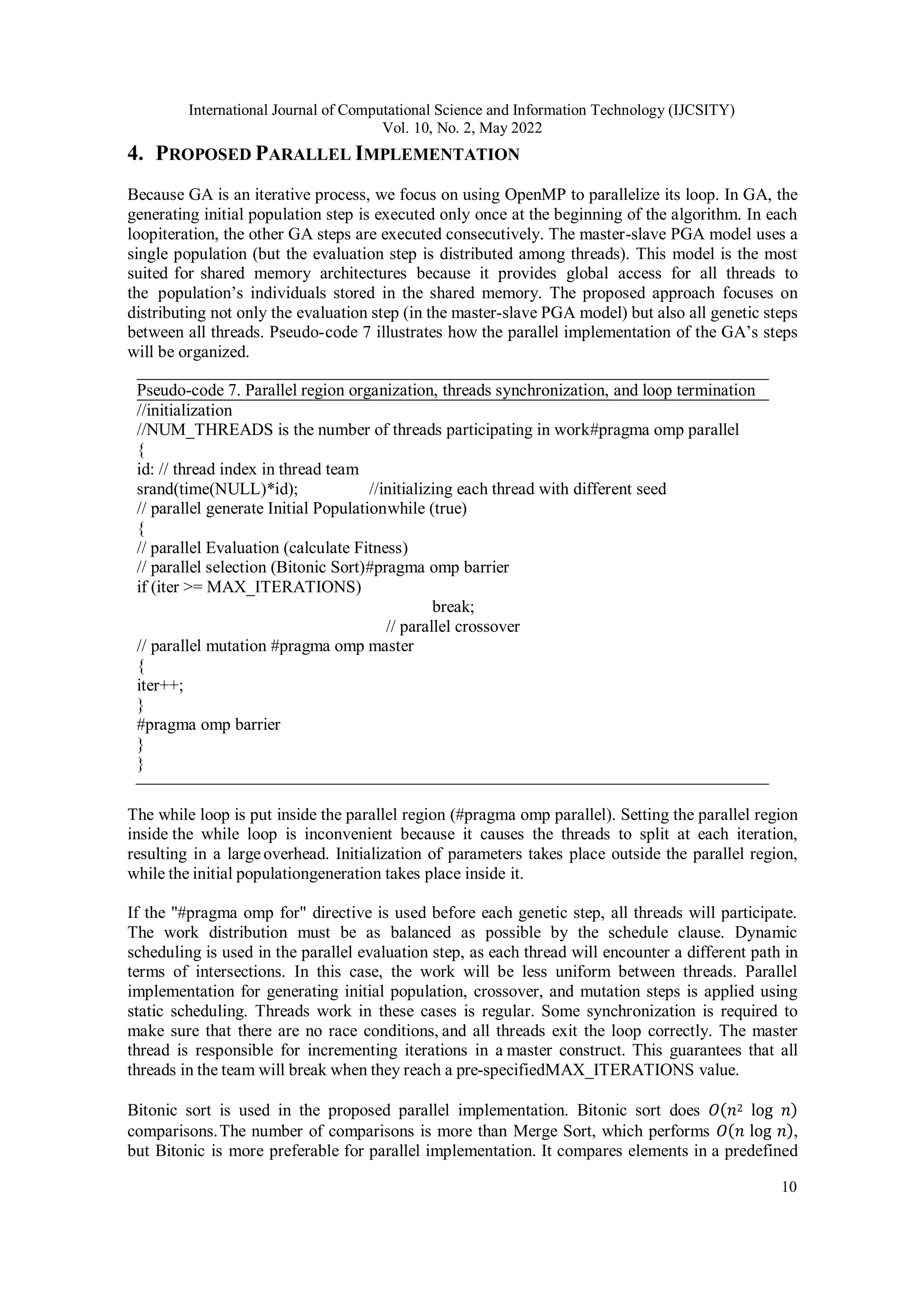
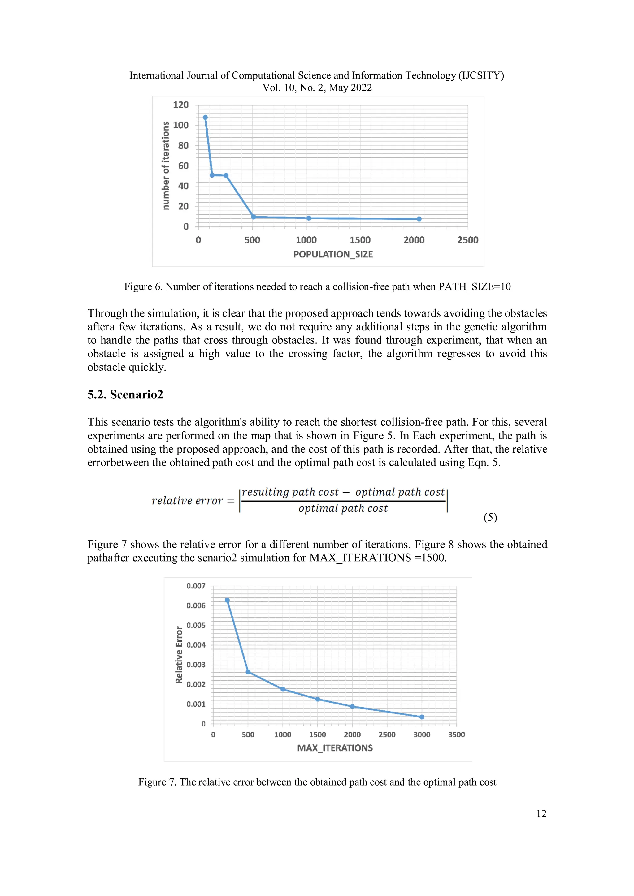
  International Journal ofComputational Science and Information Technology (IJCSITY) Vol. 10, No. 2, May 2022 11 sequence and the sequence of comparison does not depend on data. As a result, it takes less computation time in parallel implementation compared to sequential [26]. 5. SIMULATION AND EXPERIMENTAL RESULTS In this section, simulation and experimental results are introduced in three scenarios. For some parameters, the value will be the same across all experiments (SELECTION_RATE=0.4, CROSSOVER_RATE=0.5, and MUTATION_RATE=0.1). The crossing factor (𝑓𝑗) is assigned a different value for each obstacle. These values fall within the range [4.5-9.5]. The simulation isperformed on a PC with a 2.2GHz Intel Core i7-G8 processor. Figure 5. Map sample 5.1. Scenario1 The goal of this scenario is to test the algorithm's ability to find a collision-free path that avoids all obstacles on the map. We find out the number of iterations needed by the algorithm to get this path. Wedon't care about the path cost in this scenario. GA repeats its steps in a loop. In each iteration, we test the best path within the population that the algorithm has found in the current iteration. However, we test the intersection of this best path with all obstacles on the map. If this path is collision-free and does not intersect with any obstacle, we exit the loop and record the current iteration at which we exited. Scenario1 was tested on the map that is displayed in Figure 5. Figure 6 shows the number of iterations required by the proposed approaches to reach a collision-free path for PATH_SIZE=10 and different values of POPULATION_SIZE.
• 12.
  International Journal ofComputational Science and Information Technology (IJCSITY) Vol. 10, No. 2, May 2022 12 Figure 6. Number of iterations needed to reach a collision-free path when PATH_SIZE=10 Through the simulation, it is clear that the proposed approach tends towards avoiding the obstacles aftera few iterations. As a result, we do not require any additional steps in the genetic algorithm to handle the paths that cross through obstacles. It was found through experiment, that when an obstacle is assigned a high value to the crossing factor, the algorithm regresses to avoid this obstacle quickly. 5.2. Scenario2 This scenario tests the algorithm's ability to reach the shortest collision-free path. For this, several experiments are performed on the map that is shown in Figure 5. In Each experiment, the path is obtained using the proposed approach, and the cost of this path is recorded. After that, the relative errorbetween the obtained path cost and the optimal path cost is calculated using Eqn. 5. (5) Figure 7 shows the relative error for a different number of iterations. Figure 8 shows the obtained pathafter executing the senario2 simulation for MAX_ITERATIONS =1500. Figure 7. The relative error between the obtained path cost and the optimal path cost
• 13.
  International Journal ofComputational Science and Information Technology (IJCSITY) Vol. 10, No. 2, May 2022 13 Figure 8. The obtained path after executing the senario2 simulation for PATH_SIZE=8, POPULATION_SIZE =512, and MAX_ITERATIONS =1500 Through the simulation experiments, the proposed approach provides a path as close to the optimum aspossible, even if the path requires passing in a narrow area between obstacles or on an obstacle arc. This approach does not depend on specific points on the map, (mid-point between two obstacles, or obstaclevertices), to be crossable points. 5.3. Scenario3 This scenario compares the execution times of sequential and parallel algorithms. The algorithm is tested on the map that is shown in Figure 5, where there are twelve obstacles. This means much calculations and execution time are needed to evaluate paths. Table 3 shows the execution time of the sequential and the parallel algorithms for MAX_ITERATIONS=500, PATH_SIZE=8. (6) Table 3. Execution time of the sequential and parallel algorithm when PATH_SIZE=8 and MAX_ITERATIONS=500 NUM_THREADS POPULATION_SIZE Sequential Time (sec) Parallel Time (sec) Speedup 2 128 2.1436 1.1208 1.914316 256 4.298 2.24 1.919127 512 8.6662 4.518 1.918337 1024 17.4936 9.2766 1.885892 2048 35.9558 18.2686 1.968242 4 128 2.1588 0.634 3.40573 256 4.305 1.275 3.377573 512 8.5526 2.6464 3.232167 1024 17.5414 5.504 3.187353 2048 36.1944 11.2194 3.226128 8 128 2.1748 0.3946 5.512776 256 4.3194 0.83 5.205919 512 8.743 1.7548 4.98314 1024 18.5074 3.983 4.645983 2048 36.326 8.2354 4.41128
• 14.
  International Journal ofComputational Science and Information Technology (IJCSITY) Vol. 10, No. 2, May 2022 14 Figure 9. Speedup achieved by parallel implementation Through the simulation, it clearly appears that the parallel implementation achieves a reasonable acceleration relative to the number of threads. 6. CONCLUSION AND FUTURE WORK In This paper, we proposed a real-time path planner for UAVs based on genetic algorithm. An evaluation method was introduced here to reach the best path that avoids obstacles. All of the genetic stages for path planning were given in details. Three scenarios of simulation experiments were presented to prove that this approach tends towards providing a collision-free path that is close to optimum. Parallel implementation for each step was detailed using OpenMP, and the speedup was achieved to get fast path planning. For future works, the circular constructions could be used to smooth the final path. In addition, for parallel implementation, GPGPU will get more speedup. ACKNOWLEDGEMENT The authors would like to thank everyone who have extended his support for successful completion ofthis work. REFERENCES [1] Karur, K., Sharma, N., Dharmatti, C., & Siegel, J. E. (2021). A Survey of Path Planning Algorithms for Mobile Robots. Vehicles 2021, Vol. 3, Pages 448-468, 3(3), 448–468. https://doi.org/10.3390/VEHICLES3030027 [2] Pandey, A. (2017). Mobile Robot Navigation and Obstacle Avoidance Techniques: A Review. International Robotics & Automation Journal, 2(3), 96–105. https://doi.org/10.15406/iratj.2017.02.00023 [3] Zhang, H. Y., Lin, W. M., & Chen, A. X. (2018). Path planning for the mobile robot: A review. Symmetry, 10(10). https://doi.org/10.3390/sym10100450 [4] Ayawli, B. B. K., Chellali, R., Appiah, A. Y., & Kyeremeh, F. (2018). An Overview of Nature- Inspired, Conventional, and Hybrid Methods of Autonomous Vehicle Path Planning. Journal of Advanced Transportation, 2018. https://doi.org/10.1155/2018/8269698 [5] Patle, B. K., Babu L, G., Pandey, A., Parhi, D. R. K., & Jagadeesh, A. (2019). A review: On path planning strategies for navigation of mobile robot. Defence Technology, 15(4), 582–606. https://doi.org/10.1016/j.dt.2019.04.011 [6] Fu, S. Y., Han, L. W., Tian, Y., & Yang, G. S. (2012). Path planning for unmanned aerial vehicle based on genetic algorithm. Proceedings of the 11th IEEE International Conference on Cognitive
• 15.
  International Journal ofComputational Science and Information Technology (IJCSITY) Vol. 10, No. 2, May 2022 15 Informatics and Cognitive Computing, ICCI*CC 2012, 140–144. https://doi.org/10.1109/ICCI- CC.2012.6311139 [7] Turker, T., Sahingoz, O. K., & Yilmaz, G. (2015). 2D path planning for UAVs in radar threatening environment using simulated annealing algorithm. 2015 International Conference on Unmanned Aircraft Systems, ICUAS 2015, 56–61. https://doi.org/10.1109/ICUAS.2015.7152275 [8] Wang, Y., & Chen, W. (2014). Path planning and obstacle avoidance of unmanned aerial vehicle based on improved genetic algorithms. Proceedings of the 33rd Chinese Control Conference, CCC 2014, 8612– 8616. https://doi.org/10.1109/ChiCC.2014.6896446 [9] Tao, J., Zhong, C., Gao, L., & Deng, H. (2016). A study on path planning of unmanned aerial vehicle based on improved genetic algorithm. Proceedings - 2016 8th International Conference on Intelligent Human-Machine Systems and Cybernetics, IHMSC 2016, 2, 392–395. https://doi.org/10.1109/IHMSC.2016.182 [10] Özalp, N., Sahingöz, Ö. K., Ayan, U., & Ak, T. (2013). Autonomous Unmanned Aerial Vehicle Route Planning. 2013 21st Signal Processing and Communications Applications Conference, SIU 2013, 6–9. https://doi.org/10.1109/SIU.2013.6531559 [11] Basbous, B. (2019). 2D UAV Path Planning with Radar Threatening Areas using Simulated Annealing Algorithm for Event Detection. 2018 International Conference on Artificial Intelligence and Data Processing, IDAP 2018, 1–7. https://doi.org/10.1109/IDAP.2018.8620881 [12] Cakir, M. (2015). 2D path planning of UAVs with genetic algorithm in a constrained environment. 6th International Conference on Modeling, Simulation, and Applied Optimization, ICMSAO 2015 - Dedicated to the Memory of Late Ibrahim El-Sadek. https://doi.org/10.1109/ICMSAO.2015.7152235 [13] Kurgalin, S., & Borzunov, S. (2019). A practical approach to high-performance computing. A Practical Approach to High-Performance Computing. Springer International Publishing. https://doi.org/10.1007/978-3-030-27558-7 [14] Barlas, G. (2014). Multicore and GPU programming: An integrated approach. Multicore and GPU Programming: An Integrated Approach, 1–698. https://doi.org/10.1016/C2013-0-06820-X [15] Kale, V. (2019). Parallel Computing Architectures and APIs. Parallel Computing Architectures and APIs. CRC Press LLC. https://doi.org/10.1201/9781351029223 [16] Harada, T., & Alba, E. (2020). Parallel Genetic Algorithms: A Useful Survey. ACM Computing Surveys, 53(4). https://doi.org/10.1145/3400031 [17] K., R., S., B., & Mohanty, J. (2017). An overview of GA and PGA. International Journal of Computer Applications, 178(6), 7–9. https://doi.org/10.5120/ijca2017915829 [18] Talbi, E. G. (2015). Parallel evolutionary combinatorial optimization. Springer Handbook of Computational Intelligence, 1107–1125. https://doi.org/10.1007/978-3-662-43505-2_55 [19] Luque, G., & Alba, E. (2011). Parallel Models for Genetic Algorithms, (0), 15–30. https://doi.org/10.1007/978-3-642-22084-5_2 [20] Roberge, V., Tarbouchi, M., & Labonte, G. (2013). Comparison of parallel genetic algorithm and particle swarm optimization for real-time UAV path planning. IEEE Transactions on Industrial Informatics, 9(1), 132–141. https://doi.org/10.1109/TII.2012.2198665 [21] Muttillo, V., Giammatteo, P., Fiorilli, G., & Pomante, L. (2020). An OpenMP Parallel Genetic Algorithm for Design Space Exploration of Heterogeneous Multi-processor Embedded Systems. PervasiveHealth: Pervasive Computing Technologies for Healthcare, (January). https://doi.org/10.1145/3381427.3381431 [22] Herda, M. (2017). Parallel Genetic Algorithm for Capacitated P-median Problem. Procedia Engineering, 192(4), 313–317. https://doi.org/10.1016/j.proeng.2017.06.054 [23] J. Umbarkar, A., & S. Joshi, M. (2013). Dual Population Genetic Algorithm (GA) versus OpenMP GA for Multimodal Function Optimization. International Journal of Computer Applications, 64(19), 29–36. https://doi.org/10.5120/10744-5516 [24] Sahingoz, O. K. (2014). Generation of bezier curve-based flyable trajectories for multi-UAV systems with parallel genetic algorithm. Journal of Intelligent and Robotic Systems: Theory and Applications, 74(1–2), 499–511. https://doi.org/10.1007/s10846-013-9968-6 [25] Porta, J., Parapar, J., Doallo, R., Rivera, F. F., Santé, I., & Crecente, R. (2013). High performance genetic algorithm for land use planning. Computers, Environment and Urban Systems, 37(1), 45–58. https://doi.org/10.1016/j.compenvurbsys.2012.05.003 [26] Jain, M., Kumar, S., & Patle, V. . (2015). Estimation of Execution Time and Speedup for Bitonic Sorting in Sequential and Parallel Enviroment. International Journal of Computer Applications, 122(19), 32–35. https://doi.org/10.5120/21811-5139