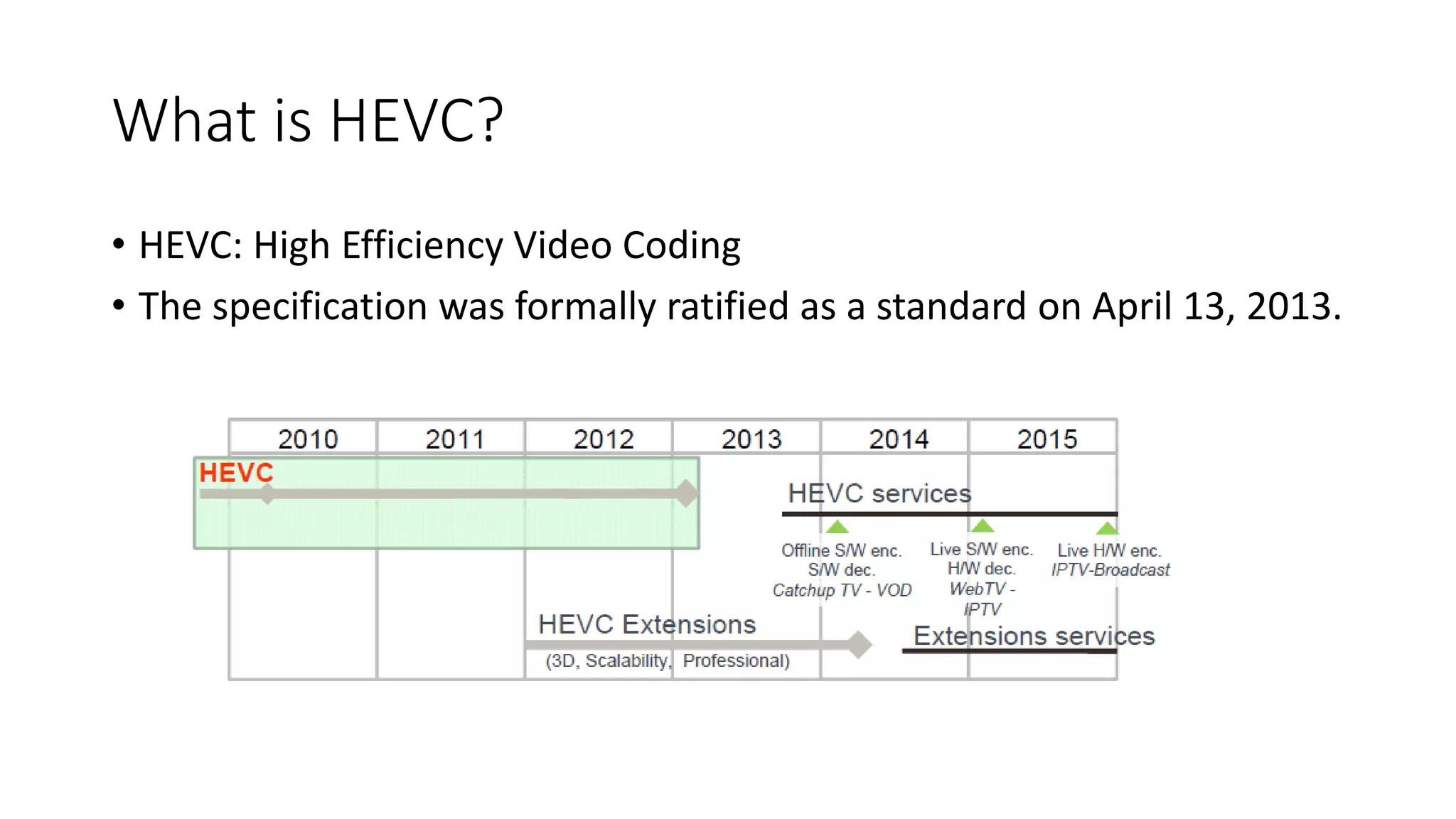
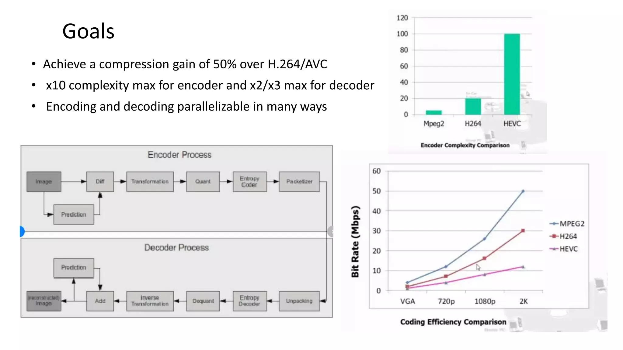
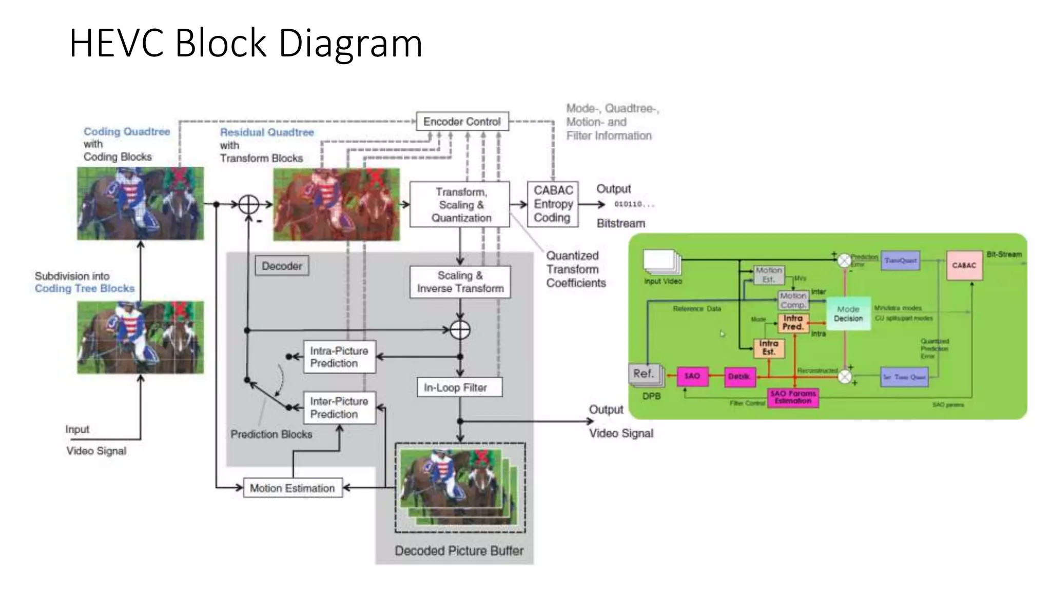
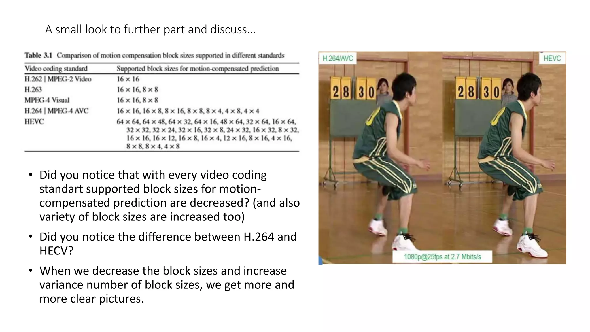
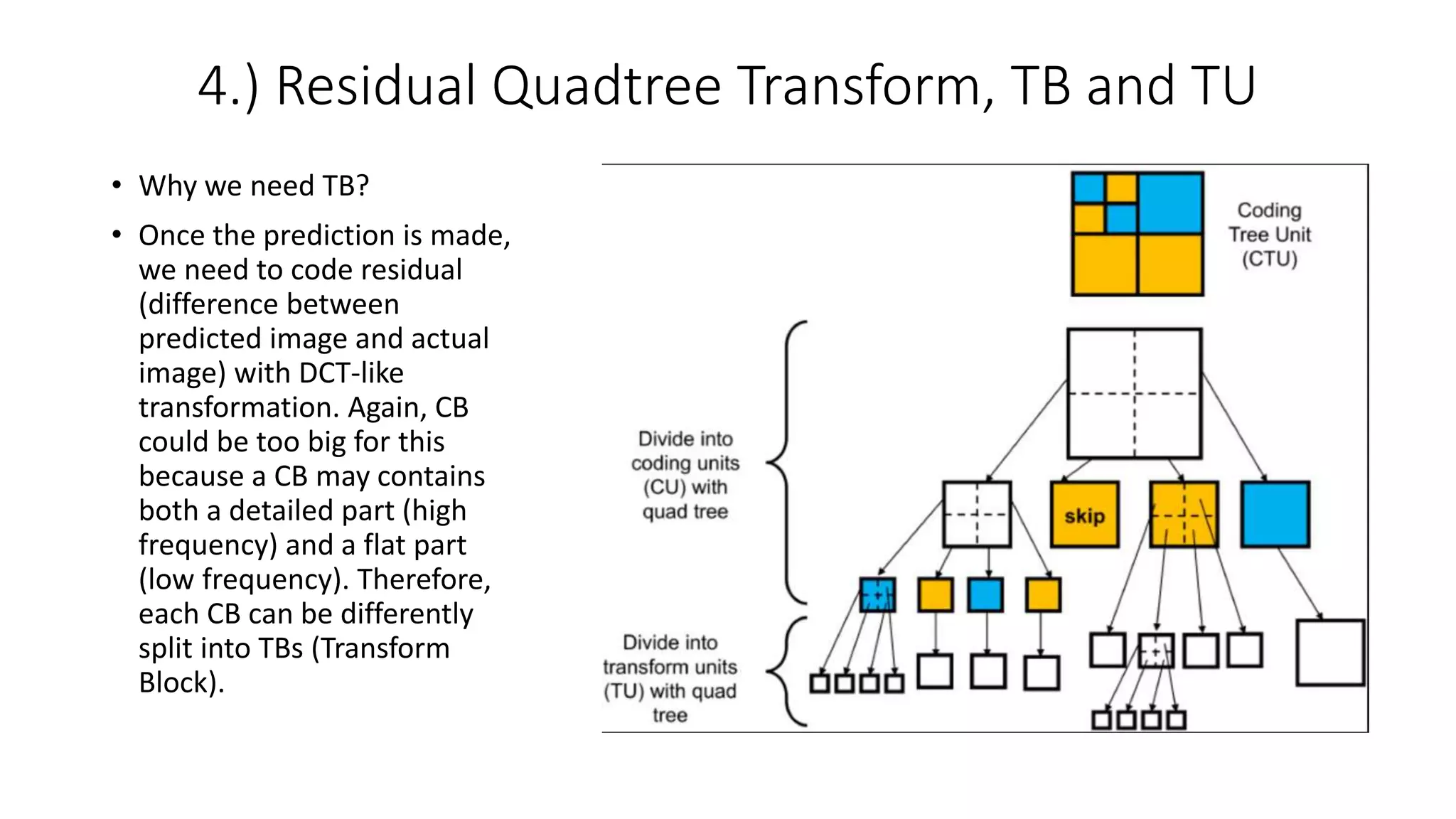
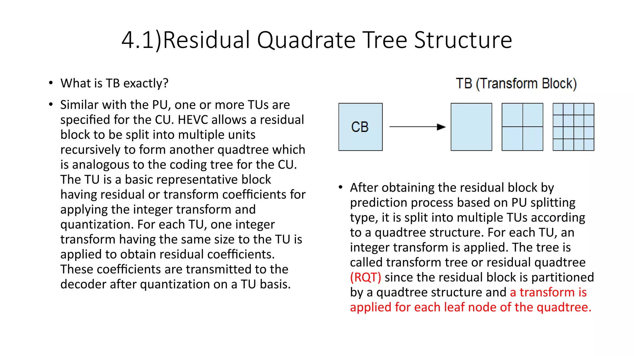
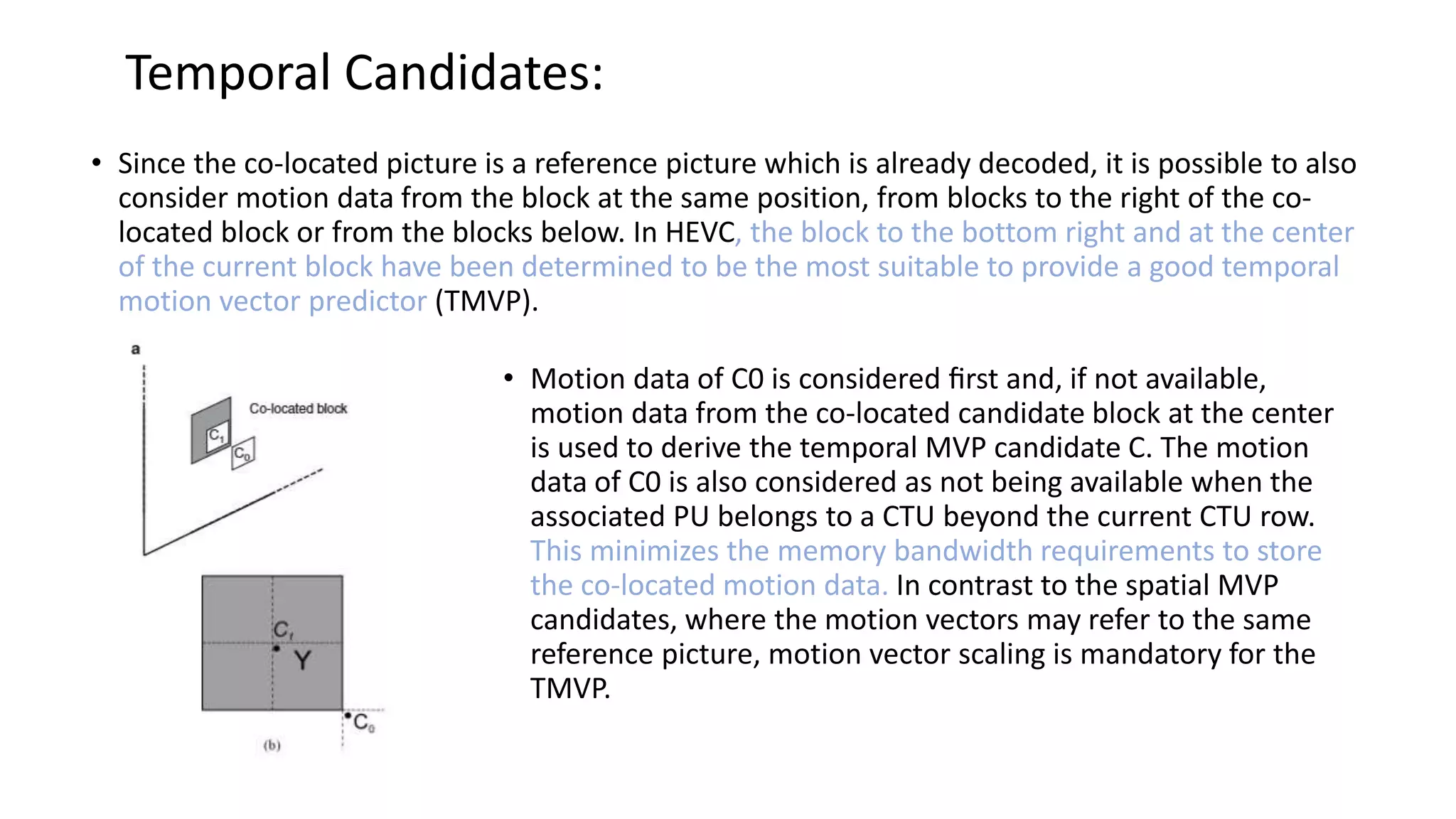
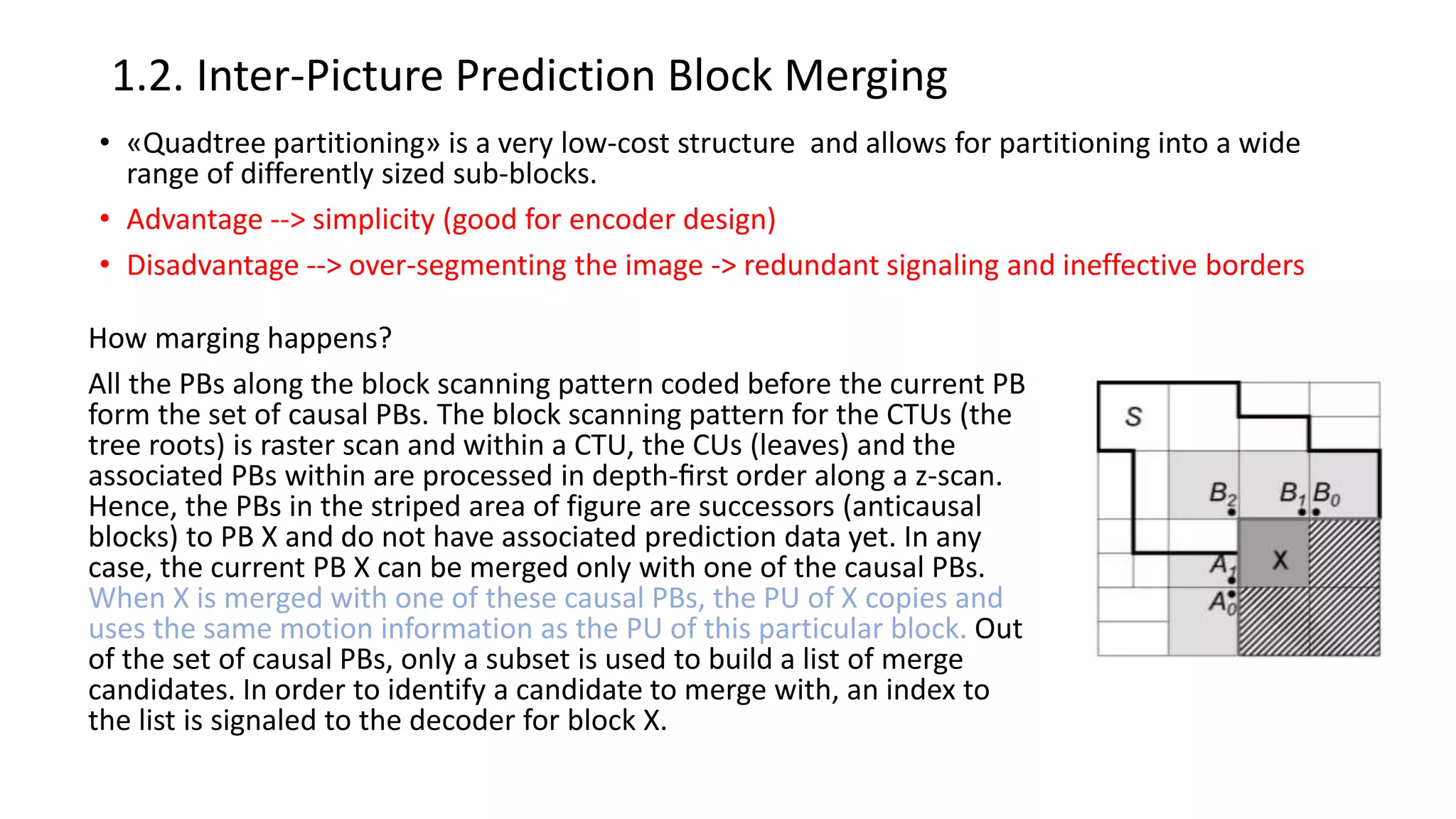
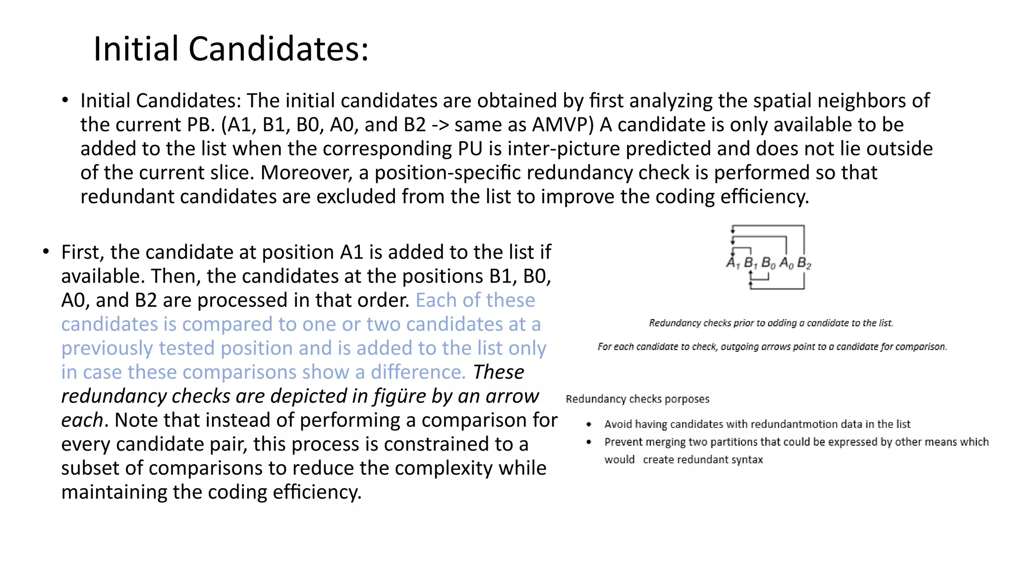
Tree structured partitioning into transform blocks and units and interpicture prediction in hevc

Multimedia Final Project Tree-Structured Partitioning into Transform Blocks and Units and Inter-picture Prediction in HEVC Laçin Acaroğlu – 05150000537 Lecturer Dr. Nükhet Özbek

What is HEVC? • HEVC: High Efficiency Video Coding • The specification was formally ratified as a standard on April 13, 2013.

Goals • Achieve a compression gain of 50% over H.264/AVC • x10 complexity max for encoder and x2/x3 max for decoder • Encoding and decoding parallelizable in many ways

Short look to H.264/AVC • Size of Macroblock • The block partitioning structure of the H.264/AVC is designed to provide more flexibility compared with the prior standards such as MPEG-2 or MPEG-4 Visual. • Assumption : 16x16 => best trade-off between between memory requirements and coding efficiency (since MPEG1) • It was found that the use of larger block sizes could increase coding efficiency significantly for high-resolution video, since the size of 16×16 is not sufficient to capture the increased spatial correlation coming from the higher resolution content.

Limited Depth of Block Partitioning : • In inter prediction of H.264/AVC, each macroblock can be processed in the following two-stage hierarchical process. • Although there are several nonsquare partitions, the block partitioning structure of H.264/AVC can be roughly related to a three-level quadtree structure which supports nodes from 4×4 to 16×16. • The way : • The macroblock 16x16 should be split and prediction should be done. • The submacroblock 8x8 should be split and prediction should be done too. • However, this kind of split and prediction combination would be inefﬁcient in HEVC due to the large number of combinations. • Unlike inter prediction, only same sizes of partitions, which can be either 4×4, 8×8, or 16×16 partitions, are allowed in a macroblock for intra prediction.

• (+) In H.264/AVC, it is possible to specify which spatial or temporal prediction scheme should be used for each macroblock. • (-) However, H.264/AVC does not allow adaptation between prediction schemes for partitions smaller than the 16×16 area. • When the inter prediction scheme is used, 4×4 transform should be used for all blocks in the macroblock if at least one block is smaller than 8×8. Even in the other case, all transform sizes should be the same within one macroblock. • This strong dependency between prediction mode and transform size and the dependency on block size make the overall design more complex to implement, especially if were to be applied to a design such as HEVC that allows more variety of block sizes.

AGENDA – Part 1 – Block Partitioning Block Partitioning for Prediction and Transform Coding  1.) Coding Tree Block and Coding Tree Unit  2.) Coding trees, CB and CU  3.) PB and PU  4.) Residual Quadtree Transform, TB and TU • 4.1)Residual Quadrate Tree Structure

A conceptually simple and very effective class of encoding algorithms are based on Lagrangian bit-allocation. The used coding parameters ‘p’ are determined by minimizing a weighted sum of the resulting distortion D and the associated number of bits R over the set A of available choices, The Lagrange parameter lamda is a constant that determines the trade-off between distortion D and the number of bits R and thus both the quality of the reconstructed video and the bit rate of the bitstream.

1.) Coding Tree Block (CTB) and CTU • HEVC divides the picture into CTUs (Coding Tree Unit). The width and height of CTU are signaled in a sequence parameter set (SPS) • CTU – Coding Tree Unit is therefore a logical unit. It usually consists of three blocks, namely luma (Y) and two chroma samples (Cb and Cr), and associated syntax elements. Each block is called CTB (Coding Tree Block).

Macroblocks and their Effect • A macroblock is a processing unit in visuals and video compression, and is based on linear block revamping. This is then subdivided into transform blocks and it is further subdivided into prediction blocks. • While increasing the size of the largest supported block size is advantageous for high-resolution video, it may have a negative impact on coding efficiency for low-resolution video, in particular if low-complexity encoder implementations are used that are not capable of evaluating all supported subpartitioning modes. For this reason, HEVC includes a flexible mechanism for partitioning video pictures into basic processing units of variable sizes. • Several studies have shown that bigger CTBs provide higher efficiency (but also higher encoding time).

Coding Tree Structure • The main advantage of introducing the coding tree structure is that in this way an elegant and unified syntax is obtained for specifying the partitioning of CTUs into blocks that are used for intra-picture prediction, motion-compensated prediction, and transform coding. • NOTE : In HEVC standard, if something is called xxxUnit, it indicates a coding logical unit which is in turn encoded into an HEVC bit stream. On the other hand, if something is called xxxBlock, it indicates a portion of video frame buffer where a process is target to.

2.) Coding trees, CB and CU • Why we need CB? • Each CTB still has the same size as CTU – 64×64, 32×32, or 16×16. Depending on a part of video frame, however, CTB may be too big to decide whether we should perform inter-picture prediction or intra-picture prediction. Thus, each CTB can be differently split into multiple CBs (Coding Blocks) and each CB becomes the decision making point of prediction type.

• Some Important Properties : • Recursive Partitioning from CTU : Let CTU size be 2N×2N where N is one of the values of 32, 16, or 8. The CTU can be a single CU or can be split into four smaller units of equal sizes of N×N, which are nodes of coding tree. • Benefits of Flexible CU Partitioning Structure : The first benefit comes from the support of CU sizes greater than the conventional 16×16 size. When the region is homogeneous, a large CU can represent the region by using a smaller number of symbols than is the case using several small blocks. Adding large size CU is an effective means to increase coding efficiency for higher resolution content. • CTU is one of the strong points of HEVC in terms of coding efficiency and adaptability for contents and applications. This ability is especially useful for low-resolution video services, which are still commonly used in the market.

• Coding efficiency difference between s64h4 and s64h2 is about 19.5% and it is also noticeable that coding efficiency difference between s64h2 and s16h2 is similar at low bit rate, but s16h2 shows better coding efficiency at high bit rate because smaller size blocks cannot be utilized for s64h2, where minimum CU size is 32 × 32 These results can be interpreted as showing that large size CU is important to increase coding efficiency in general but still small size CU should be used together to cover regions which large CU cannot be applied to successfully.

3.) PB and PU • Why we need PB? • CB is good enough for prediction type decision, but it could still be too large to store motion vectors (inter prediction) or intra prediction mode. For example, a very small object like snowfall may be moving in the middle of 8×8 CB – we want to use different MVs depending on the portion in CB. • We want to use different MVs depending on the portion in CB, that is why PB was introduced. Each CB can be split to PBs differently depending on the temporal and/or spatial predictability. For each CU, a prediction mode is signaled inside the bitstream. The prediction mode indicates whether the CU is coded using intra-picture prediction or motion-compensated prediction.

• CU is further split into one, two or four PUs • Unlike CU, PU may only be split once • Intra PU –> The basic unit to carry intra prediction information • Inter PU –> Both symmetrical and asymmetrical partitions are supported • The basic unit to carry motion information • HEVC supports eight different modes for partitioning a CU into PU’s illustrated at above.

A small look to further part and discuss… • Did you notice that with every video coding standart supported block sizes for motion- compensated prediction are decreased? (and also variety of block sizes are increased too) • Did you notice the difference between H.264 and HECV? • When we decrease the block sizes and increase variance number of block sizes, we get more and more clear pictures.

4.) Residual Quadtree Transform, TB and TU • Why we need TB? • Once the prediction is made, we need to code residual (difference between predicted image and actual image) with DCT-like transformation. Again, CB could be too big for this because a CB may contains both a detailed part (high frequency) and a flat part (low frequency). Therefore, each CB can be differently split into TBs (Transform Block).

4.1)Residual Quadrate Tree Structure • What is TB exactly? • Similar with the PU, one or more TUs are specified for the CU. HEVC allows a residual block to be split into multiple units recursively to form another quadtree which is analogous to the coding tree for the CU. The TU is a basic representative block having residual or transform coefficients for applying the integer transform and quantization. For each TU, one integer transform having the same size to the TU is applied to obtain residual coefficients. These coefficients are transmitted to the decoder after quantization on a TU basis. • After obtaining the residual block by prediction process based on PU splitting type, it is split into multiple TUs according to a quadtree structure. For each TU, an integer transform is applied. The tree is called transform tree or residual quadtree (RQT) since the residual block is partitioned by a quadtree structure and a transform is applied for each leaf node of the quadtree.

AGENDA – Part 2 – Inter-Picture Prediction • 1. Motion Data Coding • 1.1. Advanced Motion Vector Prediction (AMVP)  AMVP Candidate List Construction  Candidates • 1.2. Inter-Picture Prediction Block Merging  Merge Candidate List Construction / Candidates  Motion Data Strorage Reduction (MDSR): • 2. Fractional Sample Interpolation  Redesigned Filters  High Precision Filtering Operations  Complexity of HEVC Interpolation Filter • 3. Weighted Sample Prediction

Inter-Picture Prediction • Inter-prediction reference lists -> L0 and L1 -> Each list can store 16 references. (max different picture = 8) • Prediction modes -> 1.Merged Mode , 2.Advanced MV Each PU can use one of these modes. (İleri (1 MV) yada çift yönlü (2 MV) tahminlerde bulunabilir.) Intra-Picture Prediction : Correlation between spatially neighboring samples Inter-Picture Prediction : Temporal correlation between pictures (for derive MCP)

1.Motion Data Coding 1.1.Advanced Motion Vector Prediction : • Current block is correlated with MV of neighbouring blocks • H.264 => Wise median of 3 spatially neigbouring blocks • H.265 => Motion vector competition • Why we need motion vectors? • Motion vectors of the current block are usually correlated with the motion vectors of neighboring blocks in the current picture or in the earlier coded pictures. This is because neighboring blocks are likely to correspond to the same moving object with similar motion and the motion of the object is not likely to change abruptly over time. Consequently, using the motion vectors in neighboring blocks as predictors reduces the size of the signaled motion vector difference. The MVPs are usually derived from already decoded motion vectors from spatial neighboring blocks or from temporally neighboring blocks in the co-located picture.

AMVP Candidate List Construction • Initial design of AMVP included 5 MVPs from 3 different classes of predictors: • Three motion vectors from spatial neighbors. • The median of the three spatial predictors. • A scaled motion vector from a co-located, temporally neighboring block. • Our aim -> removing the median predictor, reducing the number of candidates in the list from five to two, fixing the candidate order in the list and reducing the number of redundancy checks • Final design AMVP candidate list construction includes: • Two spatial candidate MVPs that are derived from five spatial neighboring blocks. • One temporal candidate MVPs derived from two temporal, co-located blocks when both spatial candidate MVPs are not available or they are identical. • Zero motion vectors when the spatial, the temporal or both candidates are not available.

Candidates / Spatial Candidates: • Two spatial candidates --> A and B --> close relationship between them • Candidate A, motion data from the two blocks A0 and A1 at the bottom left corner is taken into account in a two pass approach. In the first pass, it is checked whether any of the candidate blocks contain a reference index that is equal to the reference index of the current block. The first motion vector found will be taken as candidate A. • For candidate B, the candidates B0 to B2 are checked sequentially in the same way as A0 and A1 are checked in the first pass. The second pass, however, is only performed when blocks A0 and A1 do not contain any motion information. Then, candidate A is set equal to the non-scaled candidate B, if found, and candidate B is set equal to a second, non-scaled or scaled variant of candidate B.

• Why above-left instead of below-right? Only motion vectors from spatial neighboring blocks to the left and above the current block are considered as spatial MVP candidates. This can be explained by the fact that the blocks to the right and below the current block are not yet decoded and hence, their motion data is not available. • Advantages of new design: This design allows to process A0 and A1 independently from B0, B1, and B2. The derivation of B should only be aware of the availability of both A0 and A1 in order to search for a scaled or an additional non-scaled MV derived from B0 to B2. This dependency is acceptable given that it signiﬁcantly reduces the complex motion vector scaling operations for candidate B. Reducing the number of motion vector scalings represents a signiﬁcant complexity reduction in the motion vector predictor derivation process.

Temporal Candidates: • Since the co-located picture is a reference picture which is already decoded, it is possible to also consider motion data from the block at the same position, from blocks to the right of the co- located block or from the blocks below. In HEVC, the block to the bottom right and at the center of the current block have been determined to be the most suitable to provide a good temporal motion vector predictor (TMVP). • Motion data of C0 is considered ﬁrst and, if not available, motion data from the co-located candidate block at the center is used to derive the temporal MVP candidate C. The motion data of C0 is also considered as not being available when the associated PU belongs to a CTU beyond the current CTU row. This minimizes the memory bandwidth requirements to store the co-located motion data. In contrast to the spatial MVP candidates, where the motion vectors may refer to the same reference picture, motion vector scaling is mandatory for the TMVP.

1.2. Inter-Picture Prediction Block Merging • «Quadtree partitioning» is a very low-cost structure and allows for partitioning into a wide range of differently sized sub-blocks. • Advantage --> simplicity (good for encoder design) • Disadvantage --> over-segmenting the image -> redundant signaling and ineffective borders How marging happens? All the PBs along the block scanning pattern coded before the current PB form the set of causal PBs. The block scanning pattern for the CTUs (the tree roots) is raster scan and within a CTU, the CUs (leaves) and the associated PBs within are processed in depth-ﬁrst order along a z-scan. Hence, the PBs in the striped area of figure are successors (anticausal blocks) to PB X and do not have associated prediction data yet. In any case, the current PB X can be merged only with one of the causal PBs. When X is merged with one of these causal PBs, the PU of X copies and uses the same motion information as the PU of this particular block. Out of the set of causal PBs, only a subset is used to build a list of merge candidates. In order to identify a candidate to merge with, an index to the list is signaled to the decoder for block X.

Initial Candidates: • Initial Candidates: The initial candidates are obtained by first analyzing the spatial neighbors of the current PB. (A1, B1, B0, A0, and B2 -> same as AMVP) A candidate is only available to be added to the list when the corresponding PU is inter-picture predicted and does not lie outside of the current slice. Moreover, a position-specific redundancy check is performed so that redundant candidates are excluded from the list to improve the coding efficiency. • First, the candidate at position A1 is added to the list if available. Then, the candidates at the positions B1, B0, A0, and B2 are processed in that order. Each of these candidates is compared to one or two candidates at a previously tested position and is added to the list only in case these comparisons show a difference. These redundancy checks are depicted in figüre by an arrow each. Note that instead of performing a comparison for every candidate pair, this process is constrained to a subset of comparisons to reduce the complexity while maintaining the coding efficiency.

Additional Candidates: • After the spatial and the temporal merge candidates have been added, it can happen that the list has not yet the ﬁxed length. In order to compensate for the coding efﬁciency loss that comes along with the non-length adaptive list index signaling, additional candidates are generated. • Depending on the slice type, two kind of candidates are used to fully populate the list:  Combined bi-predictive candidates  Zero motion vector candidates • In bi-predictive slices, additional candidates can be generated based on the existing ones by combining reference picture list 0 motion data of one candidate with and the list 1 motion data of another one. • When the list is still not full after adding the combined bi-predictive candidates, or for uni-predictive slices, zero motion vector candidates are calculated to complete the list. All zero motion vector candidates have one zero displacement motion vector for uni-predictive slices and two for bi-predictive slices.

Motion Data Strorage Reduction (MDSR): • The usage of the TMVP, in AMVP as well as in the merge mode, requires the storage of the motion data (including motion vectors, reference indices and coding modes) in co-located reference pictures. Considering the granularity of motion representation, the memory size needed for storing motion data could be signiﬁcant. • What HEVC do about it? --> HEVC employs motion data storage reduction (MDSR) to reduce the size of the motion data buffer and the associated memory access bandwidth by sub- sampling motion data in the reference pictures. • H.264 and H.265 difference:  While H.264/AVC is storing these information on a 4x4 block basis  HEVC uses a 16x16 block where, in case of sub-sampling a 4x4 grid, the information of the top- left 4x4 block is stored. • Due to this sub-sampling, MDSR impacts on the quality of the temporal prediction. Furthermore, there is a tight correlation between the position of the MV used in the co-located picture, and the position of the MV stored by MDSR. TMVP candidates provide the best trade off between coding efﬁciency and memory bandwidth reduction.

2. Fractional Sample Interpolation • Interpolation tasks arise naturally in the context of video coding because the true displacements of objects from one picture to another are independent of the sampling grid of cameras. • In MCP, fractional-sample accuracy is used to more accurately capture continuous motion. • The efﬁciency of MCP is limited by many factors: The spectral content of original and already reconstructed pictures, Camera noise level, Motion blur, Quantization noise in reconstructed pictures… • Similar to H.264/AVC, HEVC supports motion vectors with quarter-pixel accuracy for the luma component and one-eighth pixel accuracy for chroma components. If the motion vector has a half or quarter-pixel accuracy, samples at fractional positions need to be interpolated using the samples at integer-sample positions.

• H.264 • Obtains the quarter-sample values by (first step) obtaining the values of nearest half- pixel samples then (second step) averaging. • Bi-predictively coded block is calculated by averaging two uni-predicted blocks. • H.265 • Obtains the quarter-sample values without using such cascade steps but by instead directly applying a 7 or 8 tap filter on the integer pixels. • Keeps the samples of each one of the uni- prediction blocks at a higher accuracy and only performs rounding to input bit depth at the final stage.  it improve efficiency reducing rounding error. • Interpolation filters (number of filter taps) directly influence on «coding efficiency» and «implementation complexity». • But if number of taps increase  range of frequency increase too. (this is an advantage)

Redesigned Filters: • Increasing the number of taps can yield filters that produce desired response for a larger range of frequencies which can help to predict the corresponding frequencies in the samples to be coded. Considering modern computing capabilities, the performance of many MCP filters were evaluated in the context of HEVC and a coding efficiency/complexity trade-off was targeted during the standardization. • The basic idea is to forward transform the known integer samples to the DCT domain and inverse transform the DCT coefficients to the spatial domain using DCT basis sampled at desired fractional positions instead of integer positions. These operations can be combined into a single FIR filtering step. • Forward transform = integer samples to the DCT domain • Inverse transform = DCT coefficients to the spatial domain • Conclusion : The half-pel interpolation filter of HEVC comes closer to the desired response than the H.264/AVC filter.

High Precision Filtering Operations: • H.264/AVC Some of the intermediate values used within interpolation are shifted to lower accuracy, which introduces rounding error and reduces coding efficiency. This loss of accuracy is due to several reasons. Firstly, the half-pixel samples obtained by 6-tap FIR filter are first rounded to input bit-depth, prior to using those for obtaining the quarter-pixel samples. • H.265/HEVC • Instead of using a two-stage cascaded filtering process, HEVC interpolation filter computes the quarter-pixels directly using a 7-tap filter using the coefficients, which significantly reduces the rounding error. The second reason for reduction of accuracy in H.264/AVC motion compensation process is due to averaging in bi-prediction. In H.264/AVC, the prediction signal of the bi- predictively coded motion blocks are obtained by averaging prediction signals from two prediction lists.

Complexity of HEVC Interpolation Filter: When evaluating the complexity of a video coding algorithm there are several parameters • Memory bandwidth • Number of operations • Storage buffer size In terms of memory bandwidth, • H.264/AVC => 6-tap filter for luma sub-pixels and bilinear filter for chroma • H.265/HEVC => 7–8 tap filter for luma sub-pixels and 4-tap filter for chroma sub-pixels • This difference increases the amount of data that needs to be fetched from the reference memory.

• Thinking about worst senario could be teachable. The worst case happens when a small motion block is bi-predicted and its corresponding motion vector points to a sub-pixel position where two-dimensional filtering needs to be performed. In order to reduce the worst case memory bandwidth, HEVC introduces several restrictions. Firstly, the smallest prediction block size is fixed to be 4x8 or 8x4, instead of 4x4. In addition, these smallest block sizes of size 4x8 and 8x4 can only be predicted with uni-prediction. With these restrictions in place, the worst-case memory bandwidth of HEVC interpolation filter is around 51% higher than that of H.264/AVC. The increase in memory bandwidth is not very high for larger block sizes. For example, for a 32x32 motion block, HEVC requires around 13% increased memory bandwidth over H.264/AVC. • Longer tap filters  more operations for interpolated sample. • An H.264/AVC encoder could store only the integer and half-pel samples in the memory and generate the quarter-pixels on-the-fly during motion estimation. This would be significantly more costly in HEVC because of the complexity of generating each quarter-pixel sample on- the-fly with a 7-tap FIR filter. • An HEVC encoder could store the quarter-pixel samples in addition to integer and half-pixel samples and use those in motion estimation. Alternatively, an HEVC encoder could estimate the values of quarter-pixel samples during motion estimation by low complexity non- normative means.

3. Weighted Sample Prediction • Similar to H.264/AVC, HEVC includes a weighted prediction (WP) tool that is particularly useful for coding sequences with fades. In WP, a multiplicative weighting factor and an additive offset are applied to the motion compensated prediction. The inputs to the WP process are: • The width and the height of the luma prediction block • Prediction samples to be weighted • The prediction list utilization ﬂags • The reference indices for each list • The color component index

AGENDA – Part 3 – Experimental Study • Coding/Access Settings • Low Delay and Random Access Configuration Files . • HEVC Motion Estimation and TZ Search Algorithm • Conclusion

Coding/Access Settings • There are 3 mode exist. We will consider only two of them in this representation.

I can observe the way these two modes are performed through my own files. Note which frames are created later and how much bit is spent for them. (Also consider the GOP size) • An Low Delay config result (GOP = 4) • An Random Access config result (GOP = 8)

• By making changes to these parameters, we will find out which parameter affects the encoding process and how? • Configuration Files and Motion Search parameters :

Right now, go one step back and remember AVC. Check the example for starting. We can generate general assumption for most cases. (When all other parameters are same)

Low delay 0utputs: • QP=36, GOP Size = 4

Random Access Outputs: • QP=38, GOP Size = 8

HEVC Motion Estimation and TZ Search Algorithm • I will consider the codec (HM) in this part.

Dinlediğiniz için Teşekkürler...

Tree structured partitioning into transform blocks and units and interpicture prediction in hevc

More Related Content

Similar to Tree structured partitioning into transform blocks and units and interpicture prediction in hevc

Recently uploaded

Tree structured partitioning into transform blocks and units and interpicture prediction in hevc