Speeding up (big) data manipulation with data.table package Vasily Tolkachev Zurich University of Applied Sciences (ZHAW) Institute for Data Analysis and Process Design (IDP) vasily.tolkachev@gmail.com www.idp.zhaw.ch 21.01.2016
2 About me  Sep. 2014 – Present: Research Assistant in Statistics at  Sep. 2011 – Aug. 2014: MSc Statistics & Research Assistant at  Sep. 2008 – Aug. 2011: BSc Mathematical Economics at  https://ch.linkedin.com/in/vasily-tolkachev-20130b35
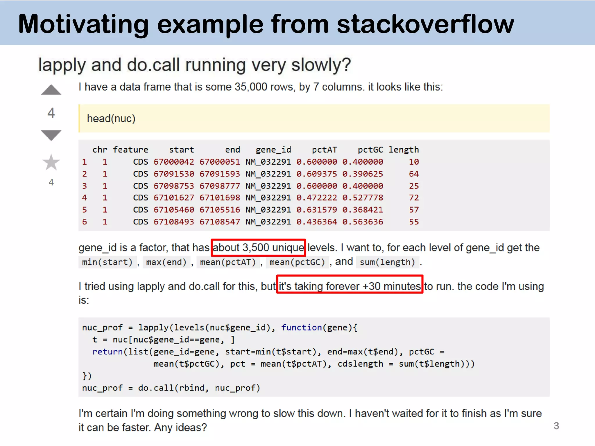
Motivating example from stackoverflow 3
dt = data.table(nuc, key="gene_id") dt[,list(A = min(start), B = max(end), C = mean(pctAT), D = mean(pctGC), E = sum(length)), by = key(dt)] # gene_id A B C D E # 1: NM_032291 67000042 67108547 0.5582567 0.4417433 283 # 2: ZZZ 67000042 67108547 0.5582567 0.4417433 283 4 data.table solution  takes ~ 3 seconds to run !  easy to program  easy to understand
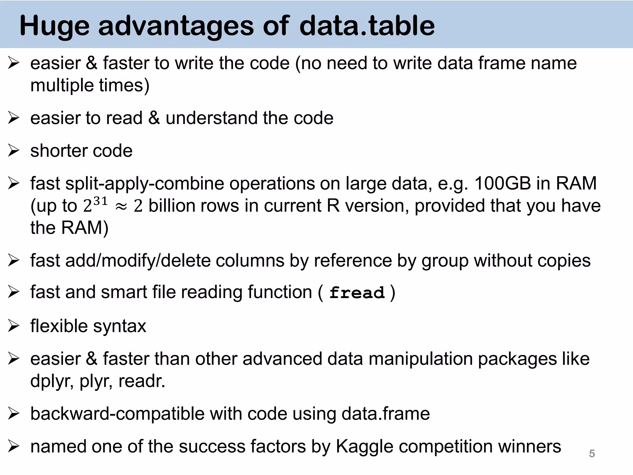
5 Huge advantages of data.table  easier & faster to write the code (no need to write data frame name multiple times)  easier to read & understand the code  shorter code  fast split-apply-combine operations on large data, e.g. 100GB in RAM (up to 231 ≈ 2 billion rows in current R version, provided that you have the RAM)  fast add/modify/delete columns by reference by group without copies  fast and smart file reading function ( fread )  flexible syntax  easier & faster than other advanced data manipulation packages like dplyr, plyr, readr.  backward-compatible with code using data.frame  named one of the success factors by Kaggle competition winners
6 How to get a lot of RAM  240 GB of RAM: https://aws.amazon.com/ec2/details/  6 TB of RAM: http://www.dell.com/us/business/p/poweredge-r920/pd
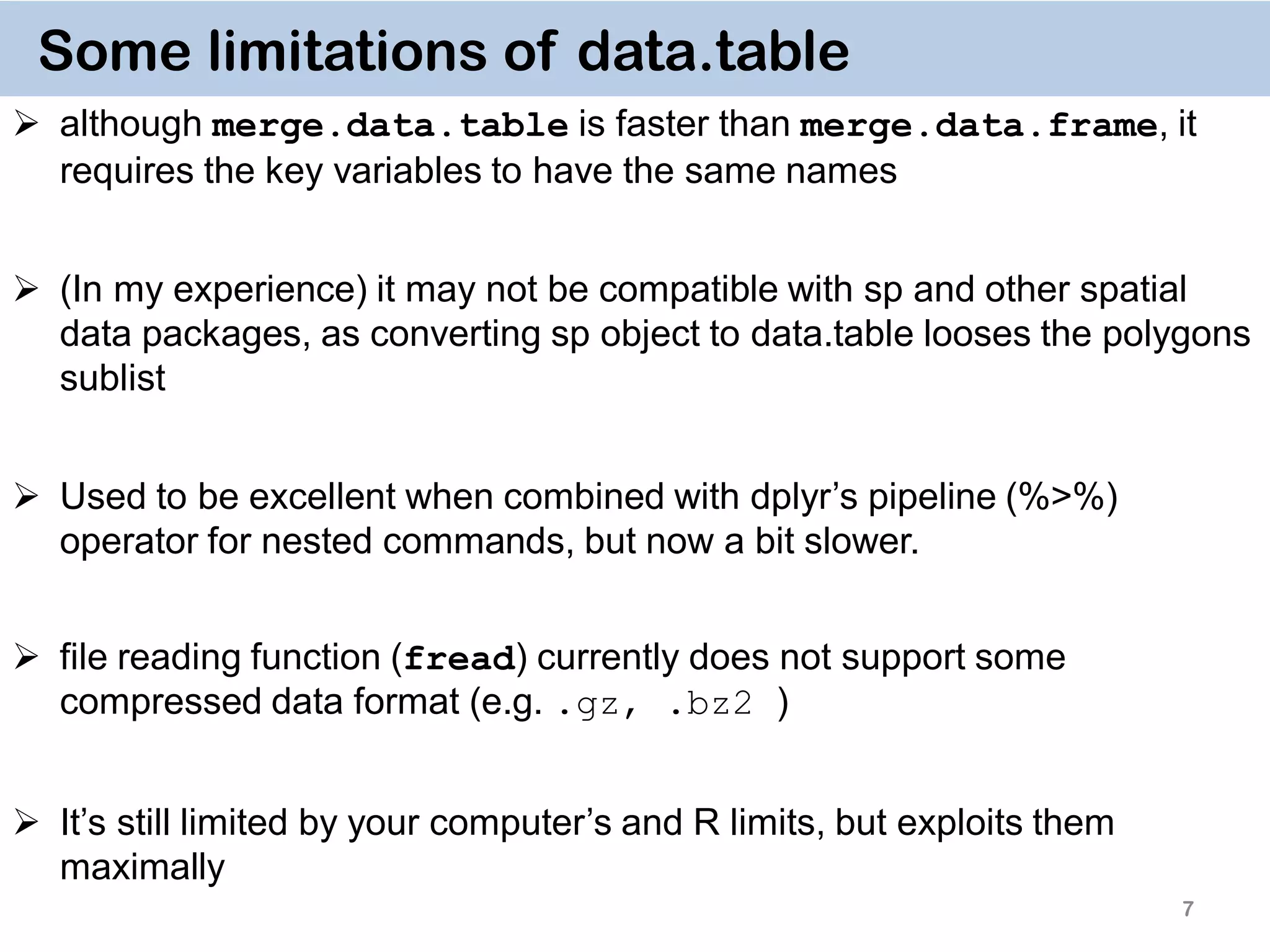
7 Some limitations of data.table  although merge.data.table is faster than merge.data.frame, it requires the key variables to have the same names  (In my experience) it may not be compatible with sp and other spatial data packages, as converting sp object to data.table looses the polygons sublist  Used to be excellent when combined with dplyr’s pipeline (%>%) operator for nested commands, but now a bit slower.  file reading function (fread) currently does not support some compressed data format (e.g. .gz, .bz2 )  It’s still limited by your computer’s and R limits, but exploits them maximally
8 General Syntax DT[i, j, by] rows or logical rule to subset obs. some function of the data To which groups apply the function Take DT, subset rows using i, then calculate j grouped by by
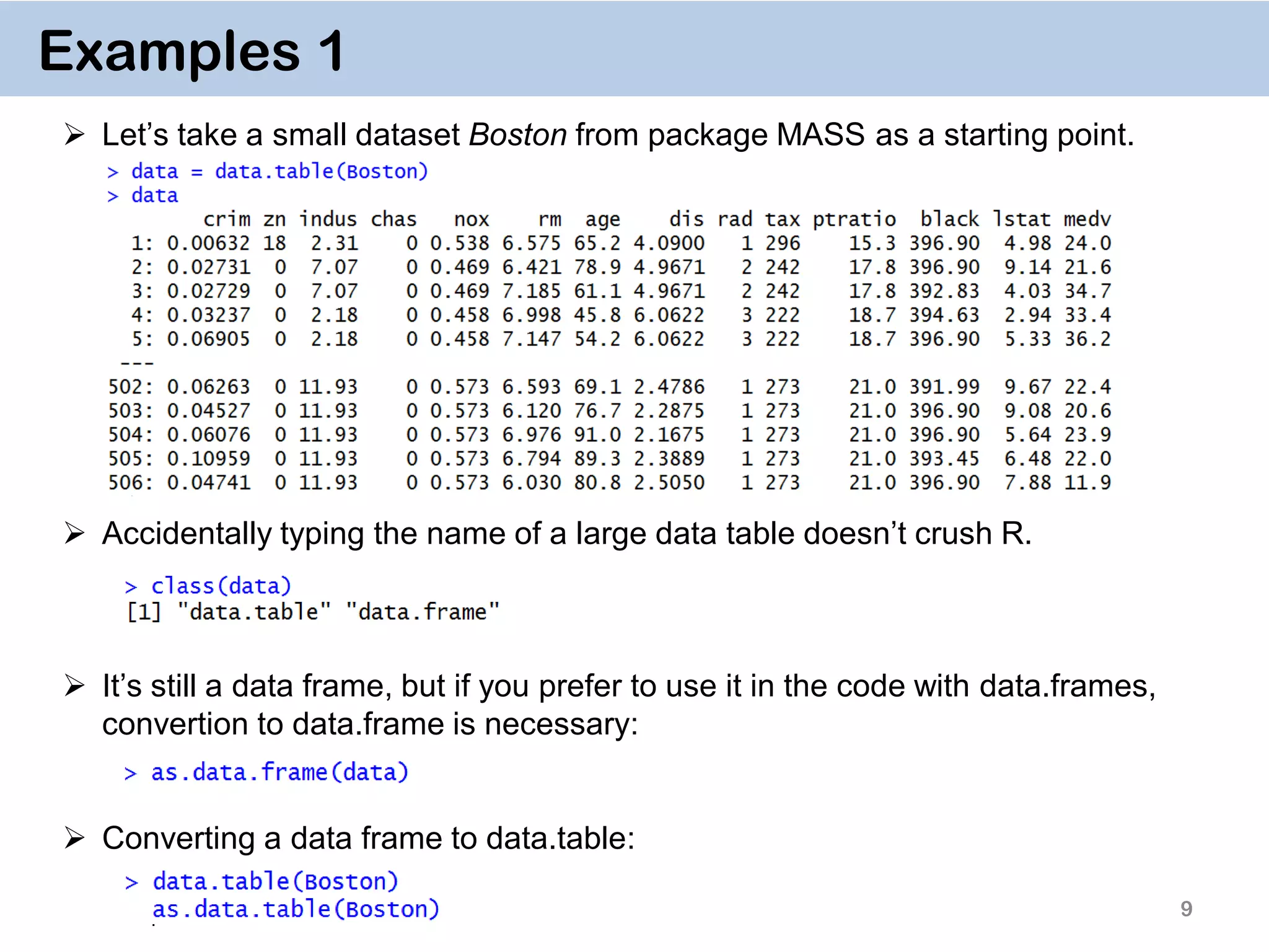
9 Examples 1  Let’s take a small dataset Boston from package MASS as a starting point.  Accidentally typing the name of a large data table doesn’t crush R.  It’s still a data frame, but if you prefer to use it in the code with data.frames, convertion to data.frame is necessary:  Converting a data frame to data.table:
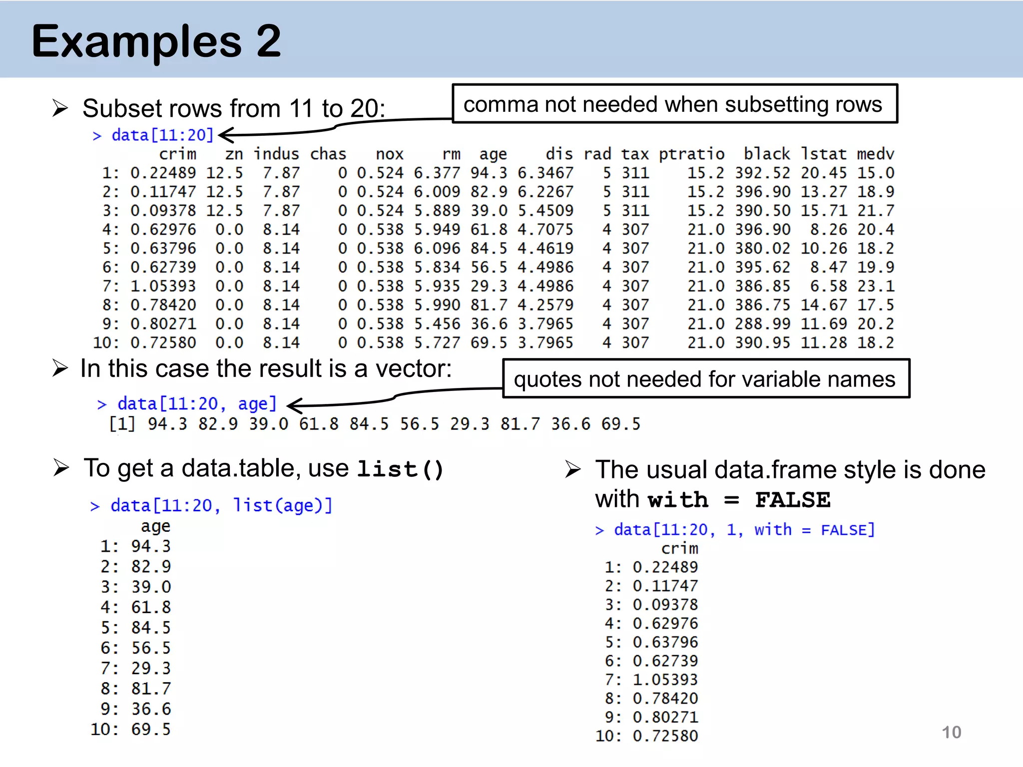
 To get a data.table, use list()  The usual data.frame style is done with with = FALSE 10 Examples 2  Subset rows from 11 to 20:  In this case the result is a vector: comma not needed when subsetting rows quotes not needed for variable names
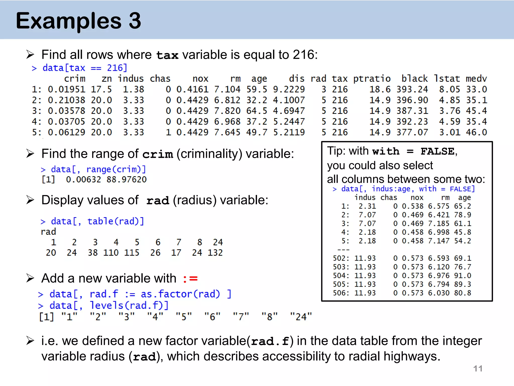
11 Examples 3  Find all rows where tax variable is equal to 216:  Find the range of crim (criminality) variable:  Display values of rad (radius) variable:  Add a new variable with :=  i.e. we defined a new factor variable(rad.f) in the data table from the integer variable radius (rad), which describes accessibility to radial highways. Tip: with with = FALSE, you could also select all columns between some two:
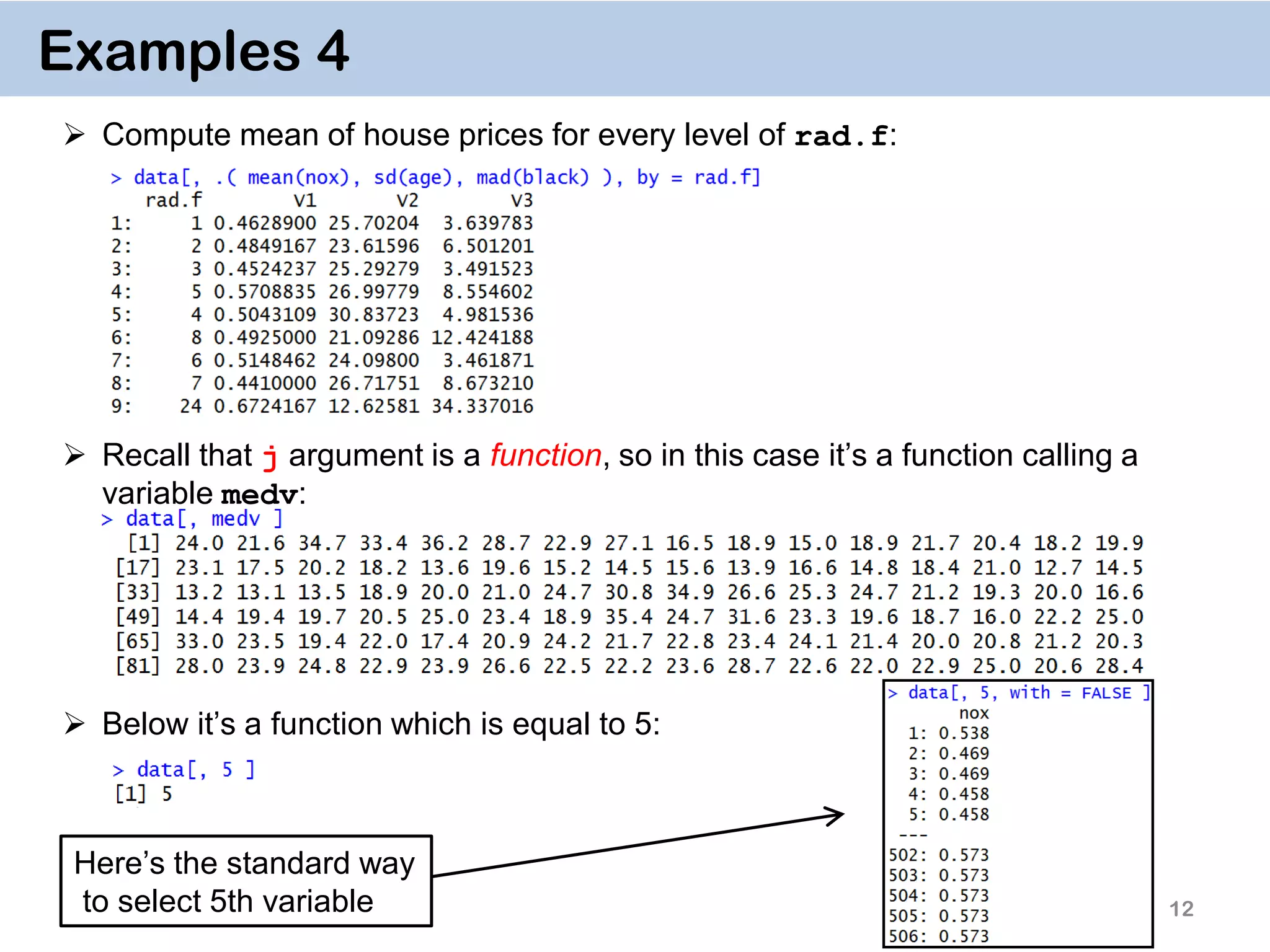
12 Examples 4  Compute mean of house prices for every level of rad.f:  Recall that j argument is a function, so in this case it’s a function calling a variable medv:  Below it’s a function which is equal to 5: Here’s the standard way to select 5th variable
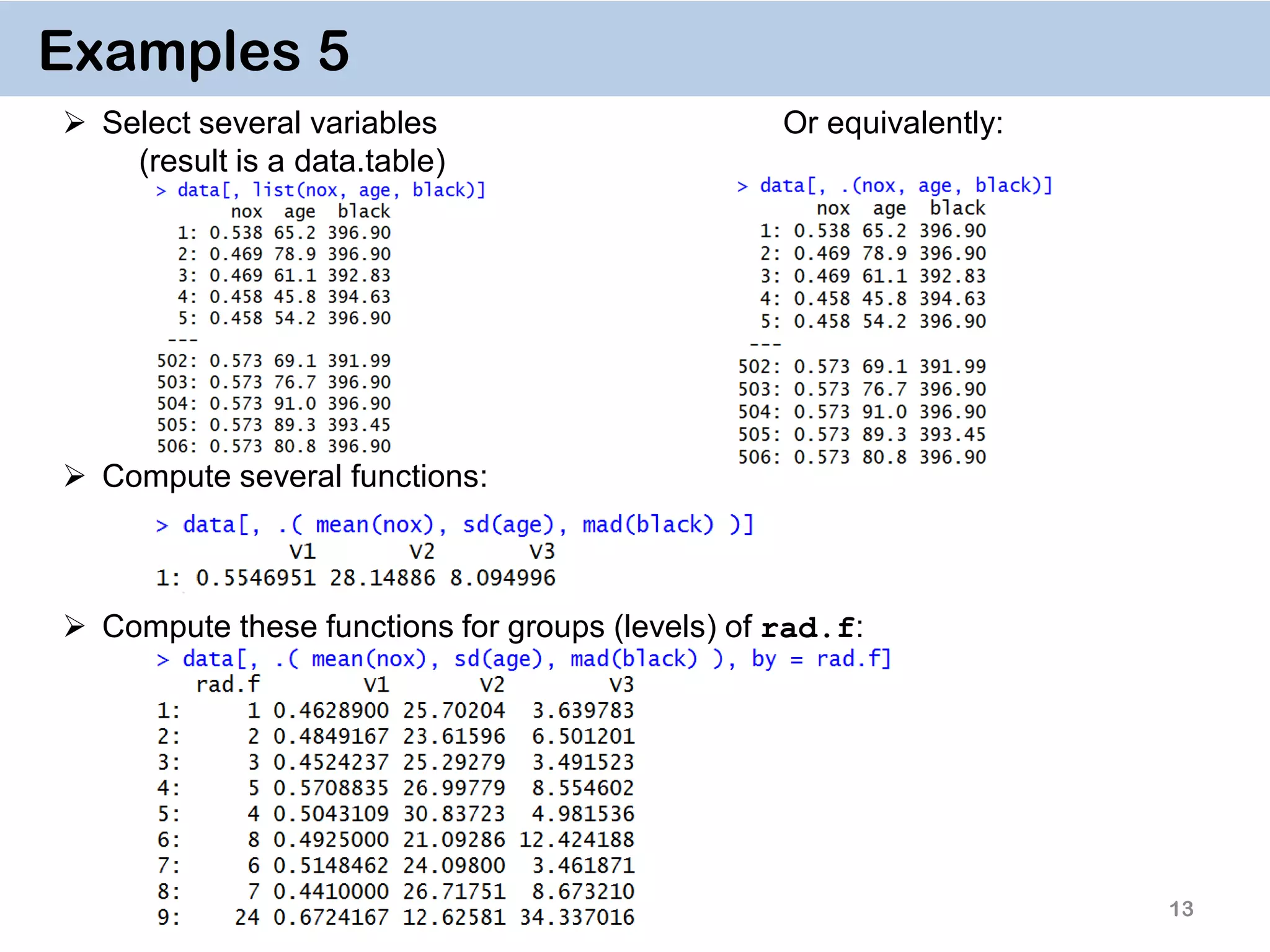
13 Examples 5  Select several variables Or equivalently: (result is a data.table)  Compute several functions:  Compute these functions for groups (levels) of rad.f:
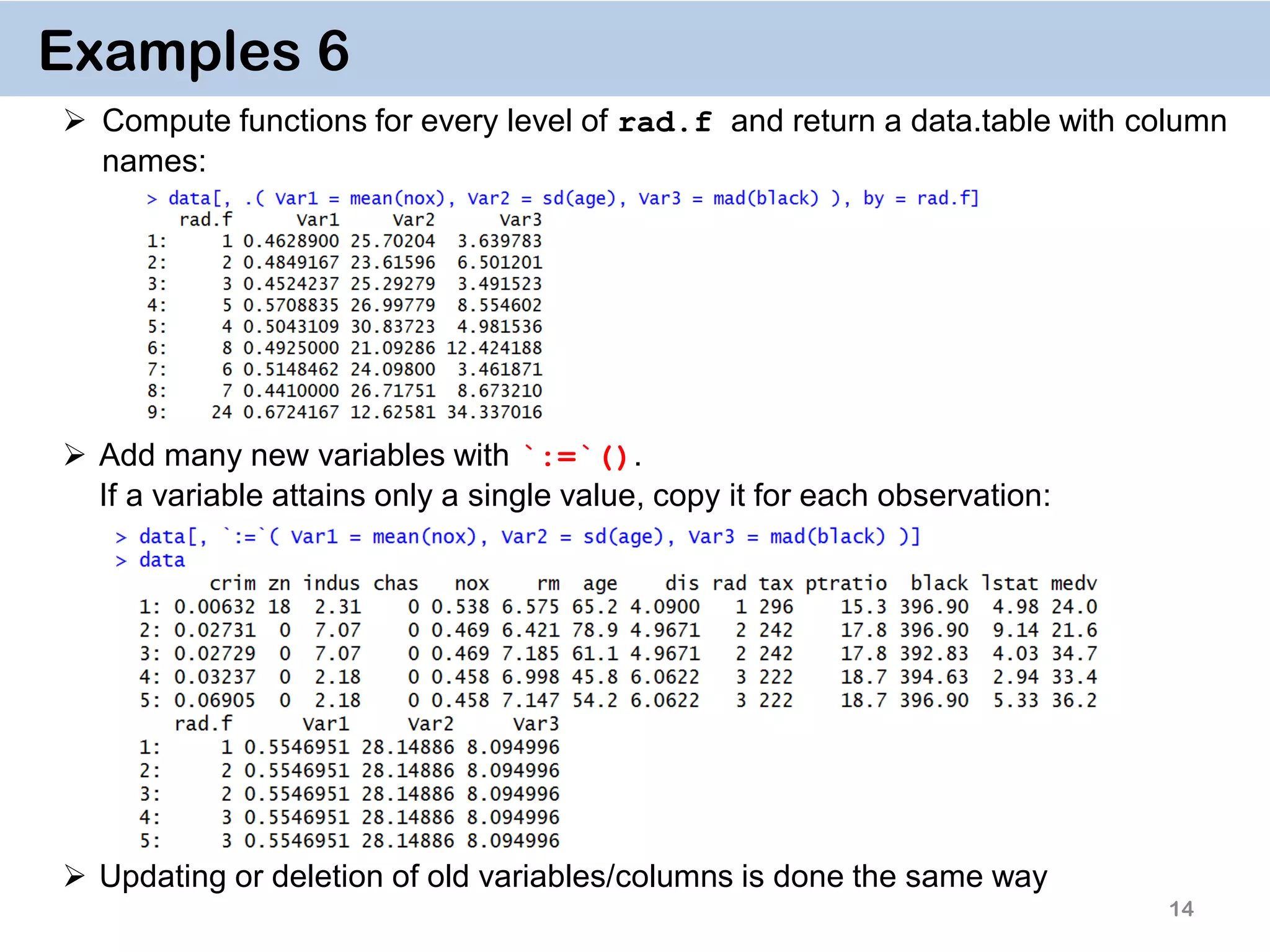
14 Examples 6  Compute functions for every level of rad.f and return a data.table with column names:  Add many new variables with `:=`(). If a variable attains only a single value, copy it for each observation:  Updating or deletion of old variables/columns is done the same way
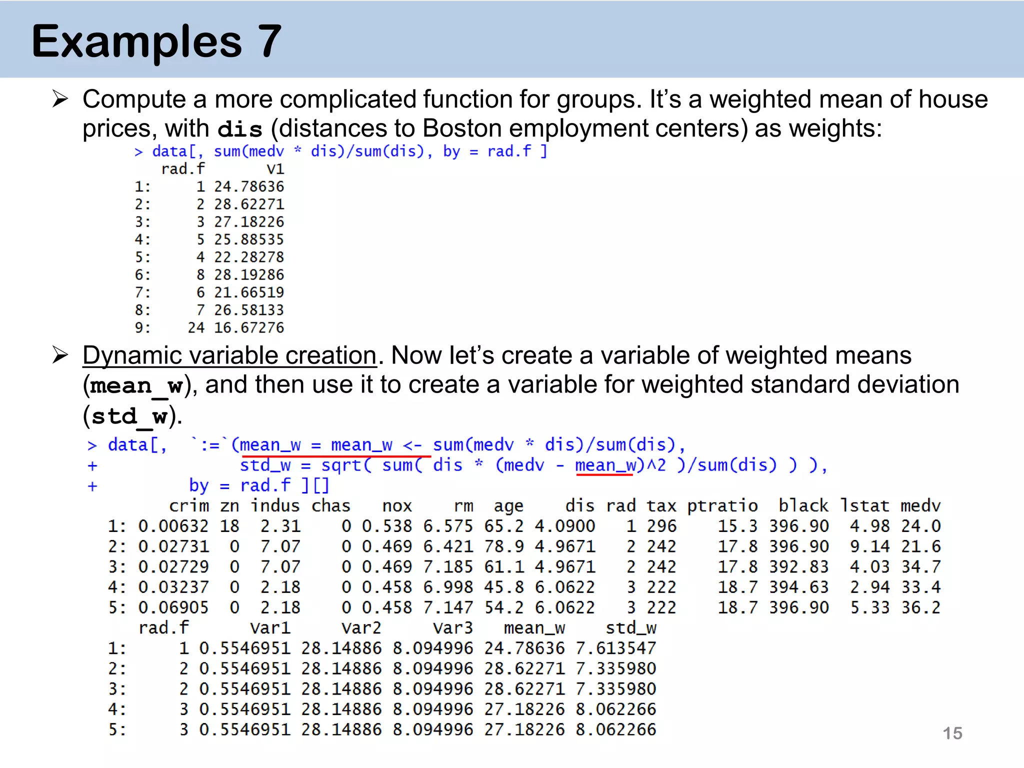
15 Examples 7  Compute a more complicated function for groups. It’s a weighted mean of house prices, with dis (distances to Boston employment centers) as weights:  Dynamic variable creation. Now let’s create a variable of weighted means (mean_w), and then use it to create a variable for weighted standard deviation (std_w).
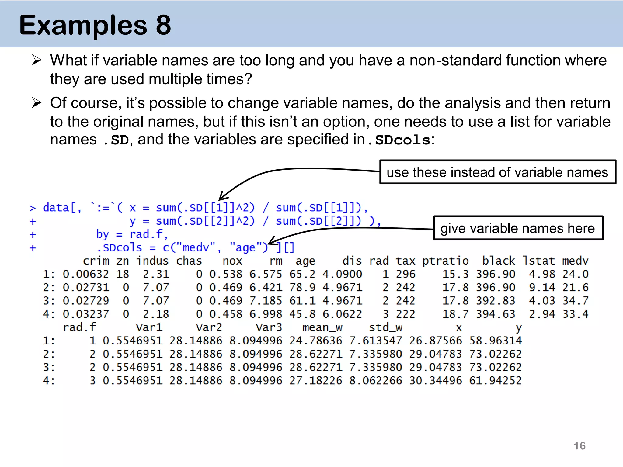
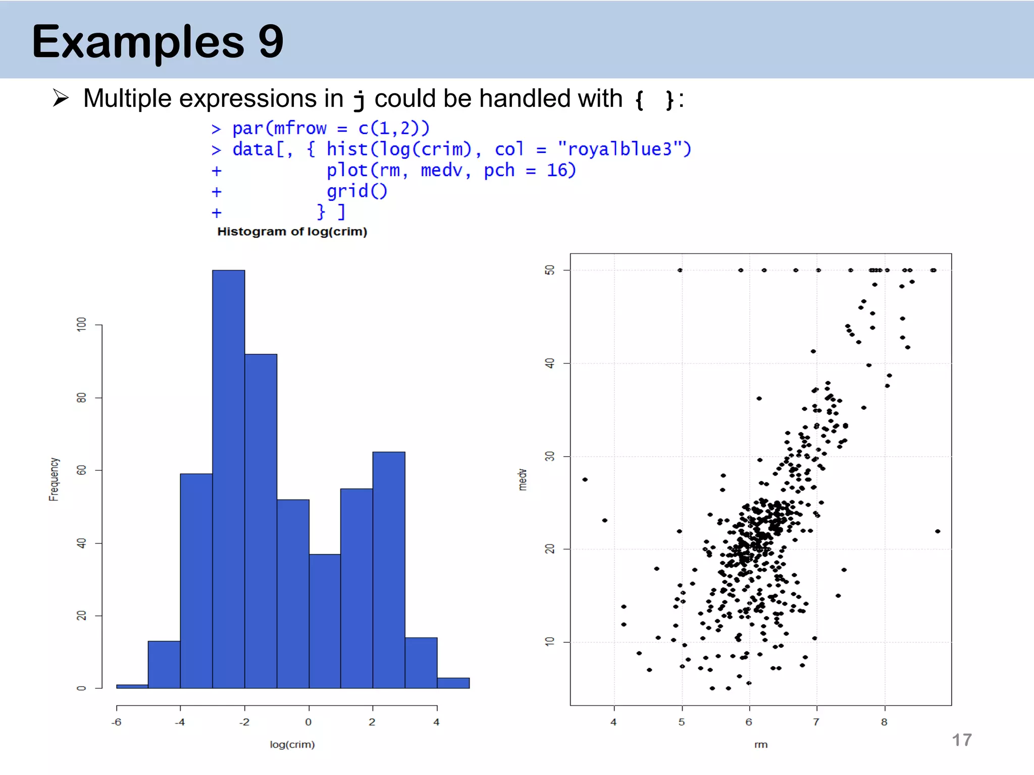
16 Examples 8  What if variable names are too long and you have a non-standard function where they are used multiple times?  Of course, it’s possible to change variable names, do the analysis and then return to the original names, but if this isn’t an option, one needs to use a list for variable names .SD, and the variables are specified in.SDcols: give variable names here use these instead of variable names
17 Examples 9  Multiple expressions in j could be handled with { }:
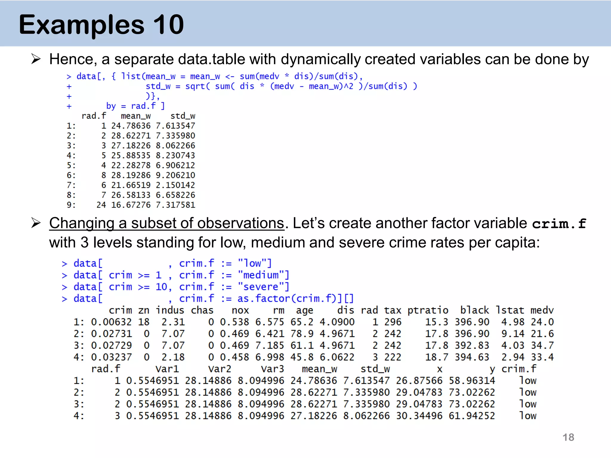
18 Examples 10  Hence, a separate data.table with dynamically created variables can be done by  Changing a subset of observations. Let’s create another factor variable crim.f with 3 levels standing for low, medium and severe crime rates per capita:
19 Examples 11. Chaining DT[i, j, by][i, j, by]  It’s a very powerful way of doing multiple operations in one command  The command for crim.f on the previous slide can thus be done by  Or in one go: data[…, …][…, …][…, …][…, …]
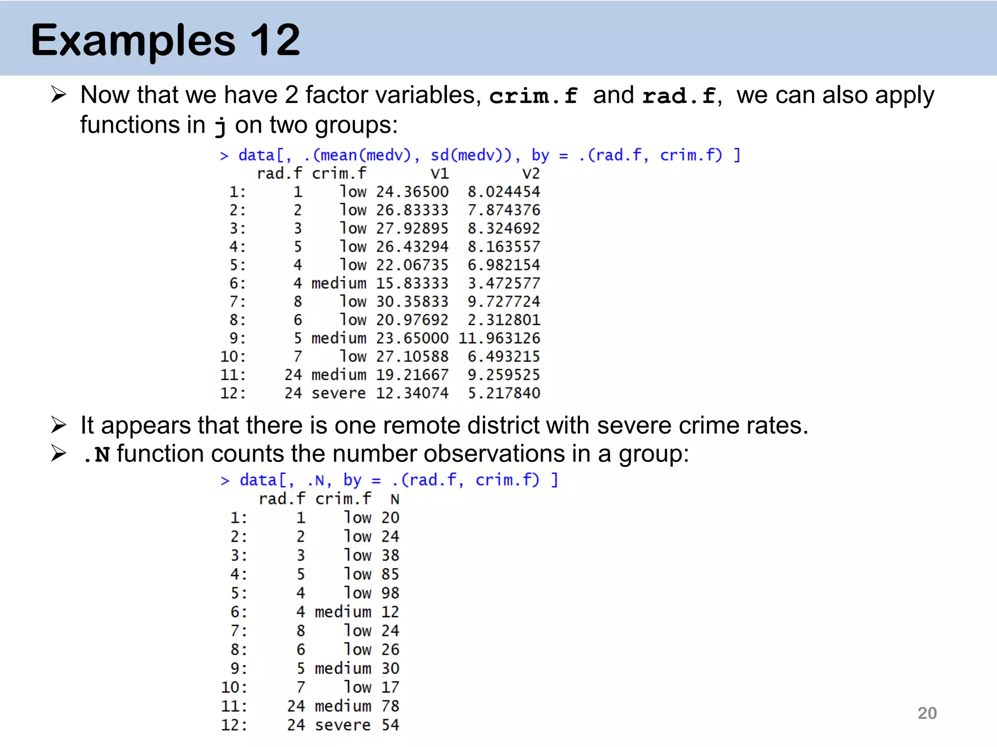
20 Examples 12  Now that we have 2 factor variables, crim.f and rad.f, we can also apply functions in j on two groups:  It appears that there is one remote district with severe crime rates.  .N function counts the number observations in a group:
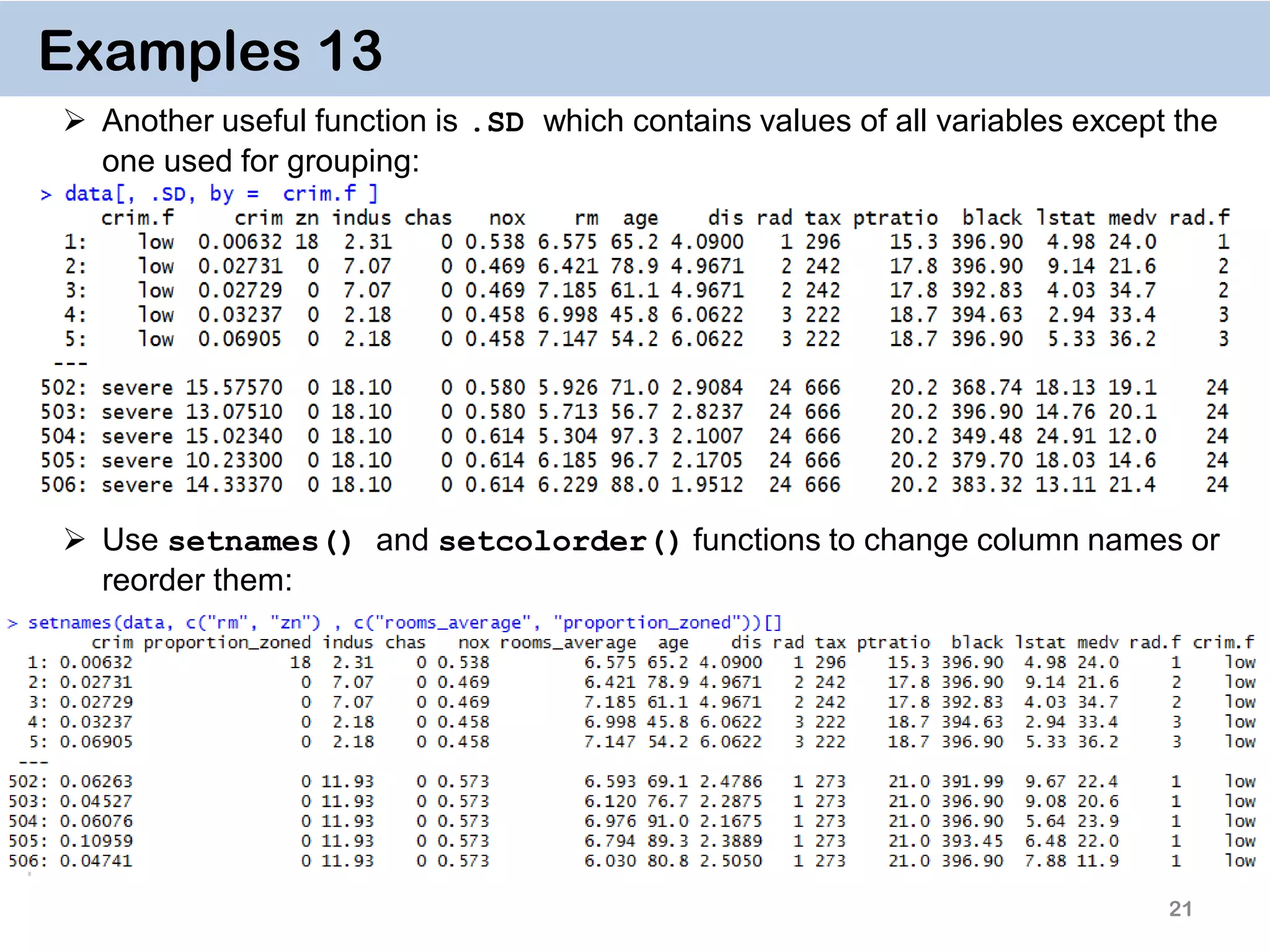
21 Examples 13  Another useful function is .SD which contains values of all variables except the one used for grouping:  Use setnames() and setcolorder() functions to change column names or reorder them:
22 Examples 14. Key on one variable  The reason why data.table works so fast is the use of keys. All observations are internally indexed by the way they are stored in RAM and sorted using Radix sort.  Any column can be set as a key (list & complex number classes not supported), and duplicate entries are allowed.  setkey(DT, colA)introduces an index for column A and sorts the data.table by it increasingly. In contrast to data.frame style, this is done without extra copies and with a very efficient memory use.  After that it’s possible to use binary search by providing index values directly data[“1”], which is 100- 1000… times faster than vector scan data[rad.f == “1”]  Setting keys is necessary for joins and significantly speeds up things for big data. However, it’s not necessary for by = aggregation.
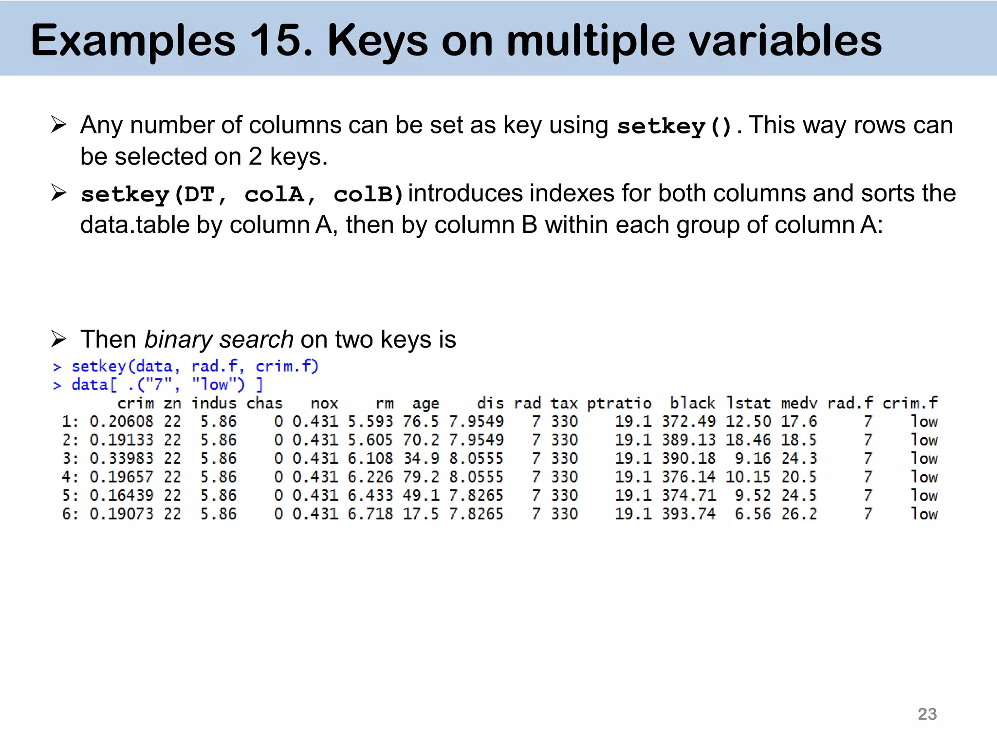
23 Examples 15. Keys on multiple variables  Any number of columns can be set as key using setkey(). This way rows can be selected on 2 keys.  setkey(DT, colA, colB)introduces indexes for both columns and sorts the data.table by column A, then by column B within each group of column A:  Then binary search on two keys is
24 Vector Scan vs. Binary Search  The reason vector scan is so inefficient is that is searches first for entries “7” in rad.f variable row-by-row, then does the same for crim.f, then takes element- wise intersection of logical vectors.  Binary search, on the other hand, searches already on sorted variables, and hence cuts the number of observations by half at each step.  Since rows of each column of data.tables have corresponding locations in RAM memory, the operations are performed in a very cache efficient manner.  In addition, since the matching row indices are obtained directly without having to create huge logical vectors (equal to the number of rows in a data.table), it is quite memory efficient as well. Vector Scan Binary search data[rad.f ==“7” & crim.f == “low”] setkey(data, rad.f, crim.f) data[ .(“7”, “low")] 𝑂(𝑛) 𝑂(log⁡( 𝑛))
25 What to avoid  Avoid read.csv function which takes hours to read in files > 1 Gb. Use fread instead. It’s a lot smarter and more efficient, e.g. it can guess the separator.  Avoid rbind which is again notoriously slow. Use rbindlist instead.  Avoid using data.frame’s vector scan inside data.table: data[ data$rad.f == "7" & data$crim.f == "low", ] (even though data.table’s vector scan is faster than data.frame’s vector scan, this slows it down.)  In general, avoid using $ inside the data.table, whether it’s for subsetting, or updating some subset of the observations: data[ data$rad.f == "7", ] = data[ data$rad.f == "7", ] + 1  For speed use := by group, don't transform() by group or cbind() afterwards  data.table used to work with dplyr well, but now it is usually slow: data %>% filter(rad == 1)
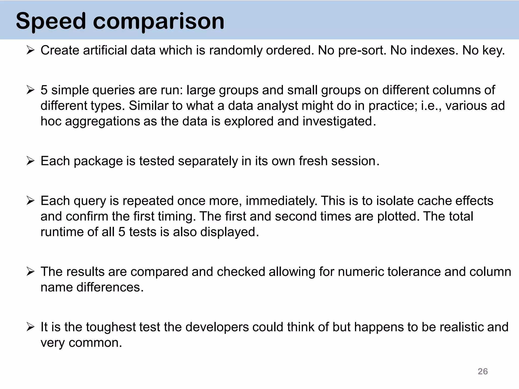
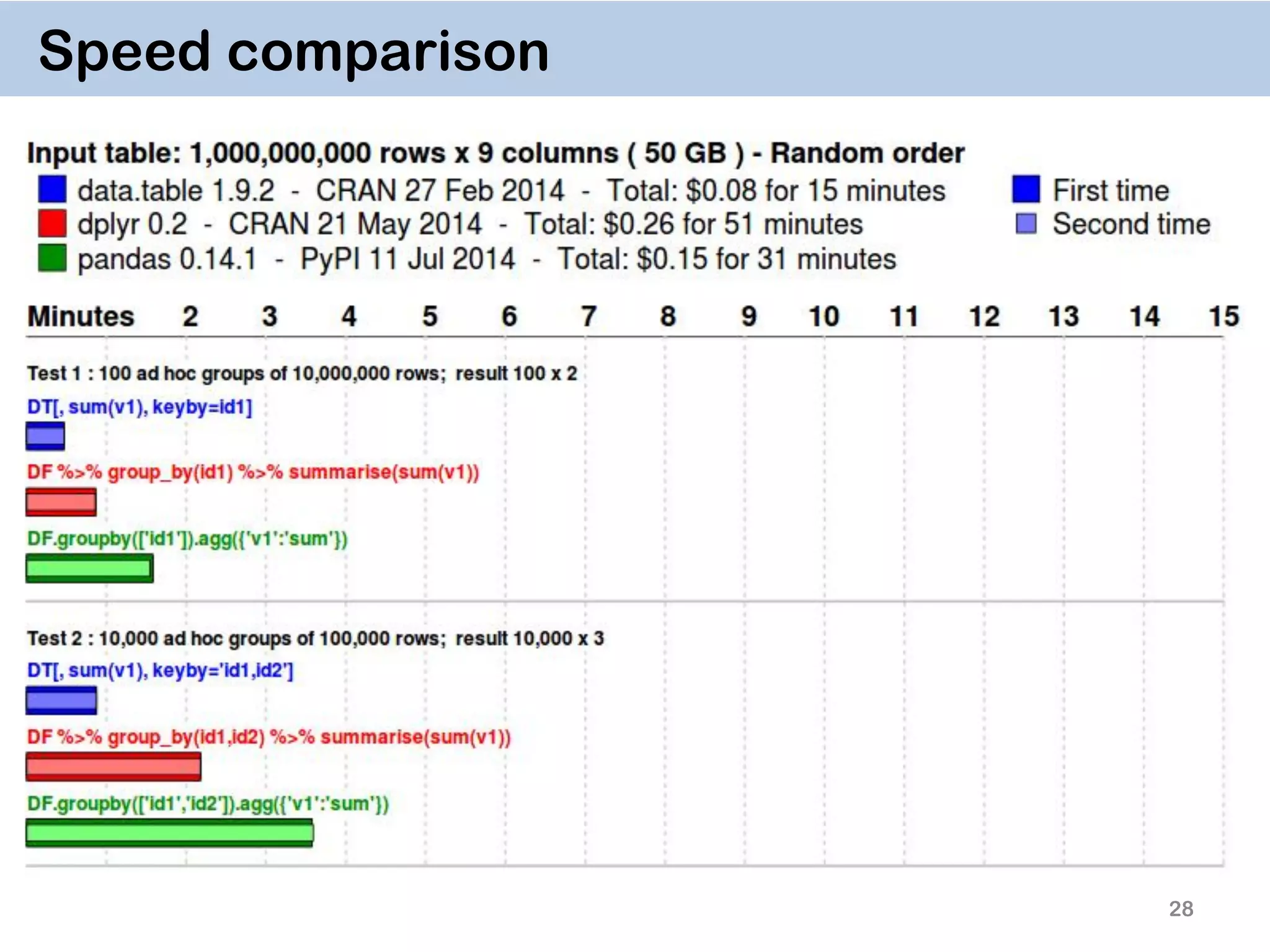
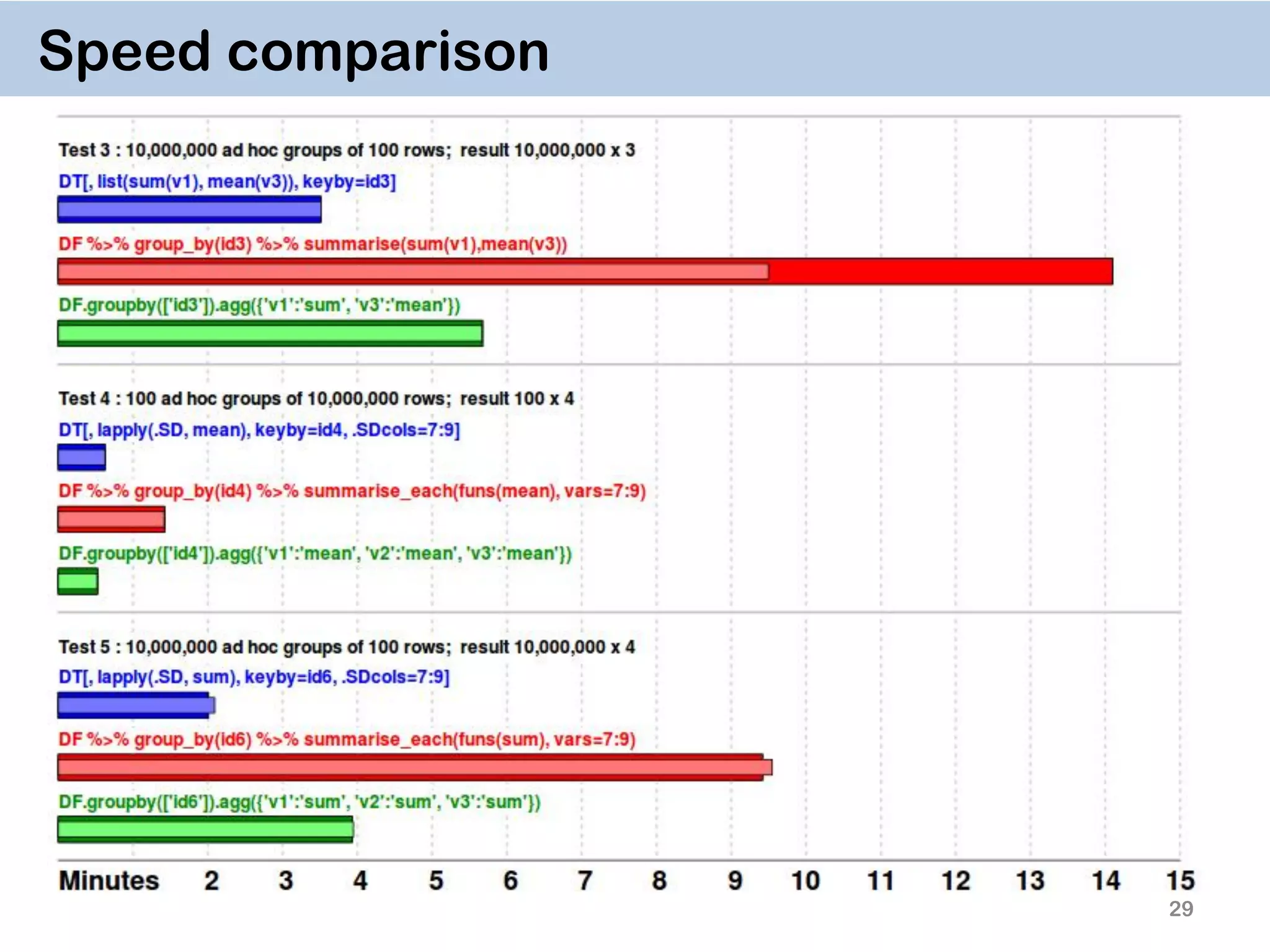
26 Speed comparison  Create artificial data which is randomly ordered. No pre-sort. No indexes. No key.  5 simple queries are run: large groups and small groups on different columns of different types. Similar to what a data analyst might do in practice; i.e., various ad hoc aggregations as the data is explored and investigated.  Each package is tested separately in its own fresh session.  Each query is repeated once more, immediately. This is to isolate cache effects and confirm the first timing. The first and second times are plotted. The total runtime of all 5 tests is also displayed.  The results are compared and checked allowing for numeric tolerance and column name differences.  It is the toughest test the developers could think of but happens to be realistic and very common.
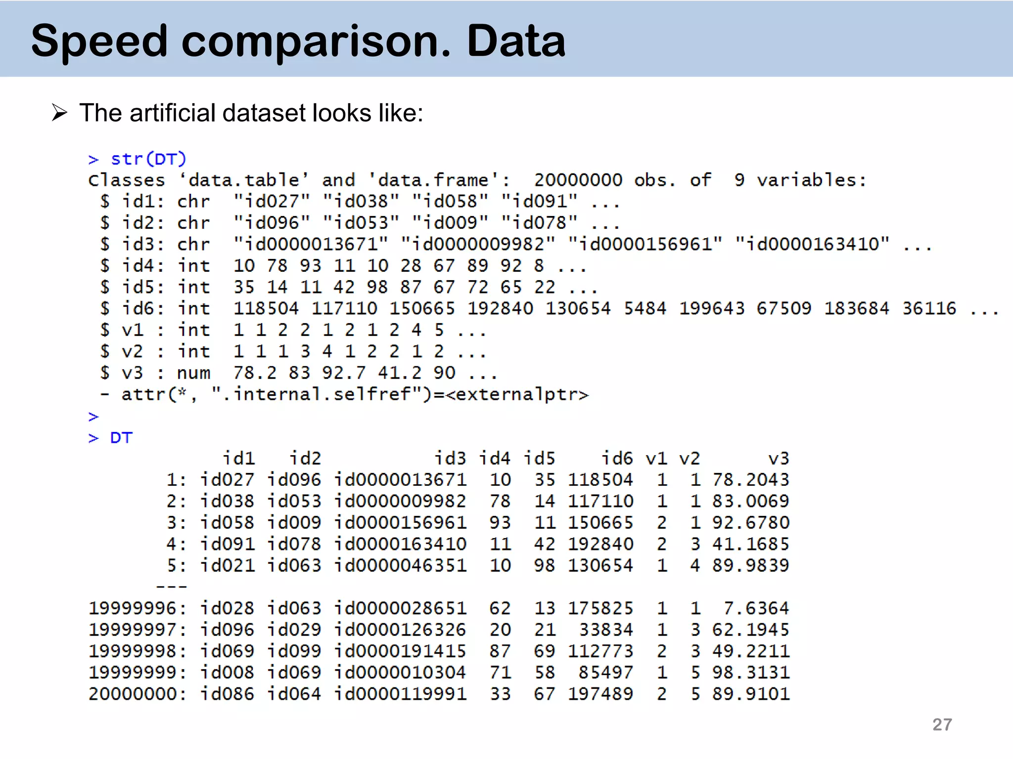
27 Speed comparison. Data  The artificial dataset looks like:
28 Speed comparison
29 Speed comparison
30 References  Matt Dowle’s data.table git account with newest vignettes. https://github.com/Rdatatable/data.table/wiki  Matt Dowle’s presentations & conference videos. https://github.com/Rdatatable/data.table/wiki/Presentations  Official introduction to data.table: https://github.com/Rdatatable/data.table/wiki/Getting-started  Why to set keys in data.table: http://stackoverflow.com/questions/20039335/what-is-the-purpose-of-setting-a- key-in-data-table  Performance comparisons to other packages: https://github.com/Rdatatable/data.table/wiki/Benchmarks-%3A-Grouping  Comprehensive data.table summary sheet: https://s3.amazonaws.com/assets.datacamp.com/img/blog/data+table+cheat+she et.pdf  An unabridged comparison of dplyr and data.table: http://stackoverflow.com/questions/21435339/data-table-vs-dplyr-can-one-do- something-well-the-other-cant-or-does-poorly/27840349#27840349
Thanks a lot for your attention and interest!

January 2016 Meetup: Speeding up (big) data manipulation with data.table package

  • 1.
    Speeding up (big) datamanipulation with data.table package Vasily Tolkachev Zurich University of Applied Sciences (ZHAW) Institute for Data Analysis and Process Design (IDP) vasily.tolkachev@gmail.com www.idp.zhaw.ch 21.01.2016
  • 2.
    2 About me  Sep.2014 – Present: Research Assistant in Statistics at  Sep. 2011 – Aug. 2014: MSc Statistics & Research Assistant at  Sep. 2008 – Aug. 2011: BSc Mathematical Economics at  https://ch.linkedin.com/in/vasily-tolkachev-20130b35
  • 3.
    Motivating example fromstackoverflow 3
  • 4.
    dt = data.table(nuc,key="gene_id") dt[,list(A = min(start), B = max(end), C = mean(pctAT), D = mean(pctGC), E = sum(length)), by = key(dt)] # gene_id A B C D E # 1: NM_032291 67000042 67108547 0.5582567 0.4417433 283 # 2: ZZZ 67000042 67108547 0.5582567 0.4417433 283 4 data.table solution  takes ~ 3 seconds to run !  easy to program  easy to understand
  • 5.
    5 Huge advantages ofdata.table  easier & faster to write the code (no need to write data frame name multiple times)  easier to read & understand the code  shorter code  fast split-apply-combine operations on large data, e.g. 100GB in RAM (up to 231 ≈ 2 billion rows in current R version, provided that you have the RAM)  fast add/modify/delete columns by reference by group without copies  fast and smart file reading function ( fread )  flexible syntax  easier & faster than other advanced data manipulation packages like dplyr, plyr, readr.  backward-compatible with code using data.frame  named one of the success factors by Kaggle competition winners
  • 6.
    6 How to geta lot of RAM  240 GB of RAM: https://aws.amazon.com/ec2/details/  6 TB of RAM: http://www.dell.com/us/business/p/poweredge-r920/pd
  • 7.
    7 Some limitations ofdata.table  although merge.data.table is faster than merge.data.frame, it requires the key variables to have the same names  (In my experience) it may not be compatible with sp and other spatial data packages, as converting sp object to data.table looses the polygons sublist  Used to be excellent when combined with dplyr’s pipeline (%>%) operator for nested commands, but now a bit slower.  file reading function (fread) currently does not support some compressed data format (e.g. .gz, .bz2 )  It’s still limited by your computer’s and R limits, but exploits them maximally
  • 8.
    8 General Syntax DT[i, j,by] rows or logical rule to subset obs. some function of the data To which groups apply the function Take DT, subset rows using i, then calculate j grouped by by
  • 9.
    9 Examples 1  Let’stake a small dataset Boston from package MASS as a starting point.  Accidentally typing the name of a large data table doesn’t crush R.  It’s still a data frame, but if you prefer to use it in the code with data.frames, convertion to data.frame is necessary:  Converting a data frame to data.table:
  • 10.
     To geta data.table, use list()  The usual data.frame style is done with with = FALSE 10 Examples 2  Subset rows from 11 to 20:  In this case the result is a vector: comma not needed when subsetting rows quotes not needed for variable names
  • 11.
    11 Examples 3  Findall rows where tax variable is equal to 216:  Find the range of crim (criminality) variable:  Display values of rad (radius) variable:  Add a new variable with :=  i.e. we defined a new factor variable(rad.f) in the data table from the integer variable radius (rad), which describes accessibility to radial highways. Tip: with with = FALSE, you could also select all columns between some two:
  • 12.
    12 Examples 4  Computemean of house prices for every level of rad.f:  Recall that j argument is a function, so in this case it’s a function calling a variable medv:  Below it’s a function which is equal to 5: Here’s the standard way to select 5th variable
  • 13.
    13 Examples 5  Selectseveral variables Or equivalently: (result is a data.table)  Compute several functions:  Compute these functions for groups (levels) of rad.f:
  • 14.
    14 Examples 6  Computefunctions for every level of rad.f and return a data.table with column names:  Add many new variables with `:=`(). If a variable attains only a single value, copy it for each observation:  Updating or deletion of old variables/columns is done the same way
  • 15.
    15 Examples 7  Computea more complicated function for groups. It’s a weighted mean of house prices, with dis (distances to Boston employment centers) as weights:  Dynamic variable creation. Now let’s create a variable of weighted means (mean_w), and then use it to create a variable for weighted standard deviation (std_w).
  • 16.
    16 Examples 8  Whatif variable names are too long and you have a non-standard function where they are used multiple times?  Of course, it’s possible to change variable names, do the analysis and then return to the original names, but if this isn’t an option, one needs to use a list for variable names .SD, and the variables are specified in.SDcols: give variable names here use these instead of variable names
  • 17.
    17 Examples 9  Multipleexpressions in j could be handled with { }:
  • 18.
    18 Examples 10  Hence,a separate data.table with dynamically created variables can be done by  Changing a subset of observations. Let’s create another factor variable crim.f with 3 levels standing for low, medium and severe crime rates per capita:
  • 19.
    19 Examples 11. Chaining DT[i,j, by][i, j, by]  It’s a very powerful way of doing multiple operations in one command  The command for crim.f on the previous slide can thus be done by  Or in one go: data[…, …][…, …][…, …][…, …]
  • 20.
    20 Examples 12  Nowthat we have 2 factor variables, crim.f and rad.f, we can also apply functions in j on two groups:  It appears that there is one remote district with severe crime rates.  .N function counts the number observations in a group:
  • 21.
    21 Examples 13  Anotheruseful function is .SD which contains values of all variables except the one used for grouping:  Use setnames() and setcolorder() functions to change column names or reorder them:
  • 22.
    22 Examples 14. Keyon one variable  The reason why data.table works so fast is the use of keys. All observations are internally indexed by the way they are stored in RAM and sorted using Radix sort.  Any column can be set as a key (list & complex number classes not supported), and duplicate entries are allowed.  setkey(DT, colA)introduces an index for column A and sorts the data.table by it increasingly. In contrast to data.frame style, this is done without extra copies and with a very efficient memory use.  After that it’s possible to use binary search by providing index values directly data[“1”], which is 100- 1000… times faster than vector scan data[rad.f == “1”]  Setting keys is necessary for joins and significantly speeds up things for big data. However, it’s not necessary for by = aggregation.
  • 23.
    23 Examples 15. Keyson multiple variables  Any number of columns can be set as key using setkey(). This way rows can be selected on 2 keys.  setkey(DT, colA, colB)introduces indexes for both columns and sorts the data.table by column A, then by column B within each group of column A:  Then binary search on two keys is
  • 24.
    24 Vector Scan vs.Binary Search  The reason vector scan is so inefficient is that is searches first for entries “7” in rad.f variable row-by-row, then does the same for crim.f, then takes element- wise intersection of logical vectors.  Binary search, on the other hand, searches already on sorted variables, and hence cuts the number of observations by half at each step.  Since rows of each column of data.tables have corresponding locations in RAM memory, the operations are performed in a very cache efficient manner.  In addition, since the matching row indices are obtained directly without having to create huge logical vectors (equal to the number of rows in a data.table), it is quite memory efficient as well. Vector Scan Binary search data[rad.f ==“7” & crim.f == “low”] setkey(data, rad.f, crim.f) data[ .(“7”, “low")] 𝑂(𝑛) 𝑂(log⁡( 𝑛))
  • 25.
    25 What to avoid Avoid read.csv function which takes hours to read in files > 1 Gb. Use fread instead. It’s a lot smarter and more efficient, e.g. it can guess the separator.  Avoid rbind which is again notoriously slow. Use rbindlist instead.  Avoid using data.frame’s vector scan inside data.table: data[ data$rad.f == "7" & data$crim.f == "low", ] (even though data.table’s vector scan is faster than data.frame’s vector scan, this slows it down.)  In general, avoid using $ inside the data.table, whether it’s for subsetting, or updating some subset of the observations: data[ data$rad.f == "7", ] = data[ data$rad.f == "7", ] + 1  For speed use := by group, don't transform() by group or cbind() afterwards  data.table used to work with dplyr well, but now it is usually slow: data %>% filter(rad == 1)
  • 26.
    26 Speed comparison  Createartificial data which is randomly ordered. No pre-sort. No indexes. No key.  5 simple queries are run: large groups and small groups on different columns of different types. Similar to what a data analyst might do in practice; i.e., various ad hoc aggregations as the data is explored and investigated.  Each package is tested separately in its own fresh session.  Each query is repeated once more, immediately. This is to isolate cache effects and confirm the first timing. The first and second times are plotted. The total runtime of all 5 tests is also displayed.  The results are compared and checked allowing for numeric tolerance and column name differences.  It is the toughest test the developers could think of but happens to be realistic and very common.
  • 27.
    27 Speed comparison. Data The artificial dataset looks like:
  • 28.
  • 29.
  • 30.
    30 References  Matt Dowle’sdata.table git account with newest vignettes. https://github.com/Rdatatable/data.table/wiki  Matt Dowle’s presentations & conference videos. https://github.com/Rdatatable/data.table/wiki/Presentations  Official introduction to data.table: https://github.com/Rdatatable/data.table/wiki/Getting-started  Why to set keys in data.table: http://stackoverflow.com/questions/20039335/what-is-the-purpose-of-setting-a- key-in-data-table  Performance comparisons to other packages: https://github.com/Rdatatable/data.table/wiki/Benchmarks-%3A-Grouping  Comprehensive data.table summary sheet: https://s3.amazonaws.com/assets.datacamp.com/img/blog/data+table+cheat+she et.pdf  An unabridged comparison of dplyr and data.table: http://stackoverflow.com/questions/21435339/data-table-vs-dplyr-can-one-do- something-well-the-other-cant-or-does-poorly/27840349#27840349
  • 31.
    Thanks a lotfor your attention and interest!