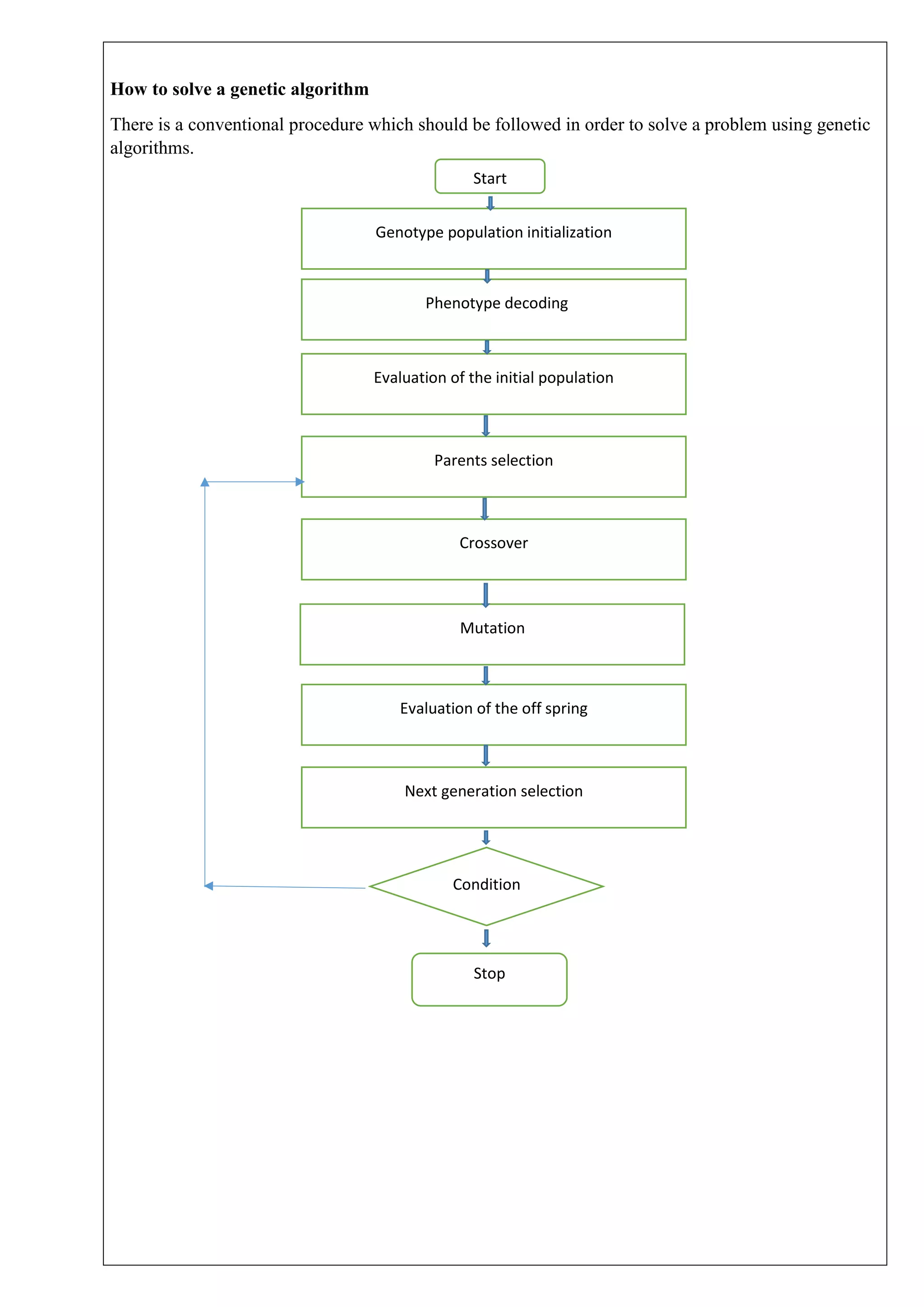
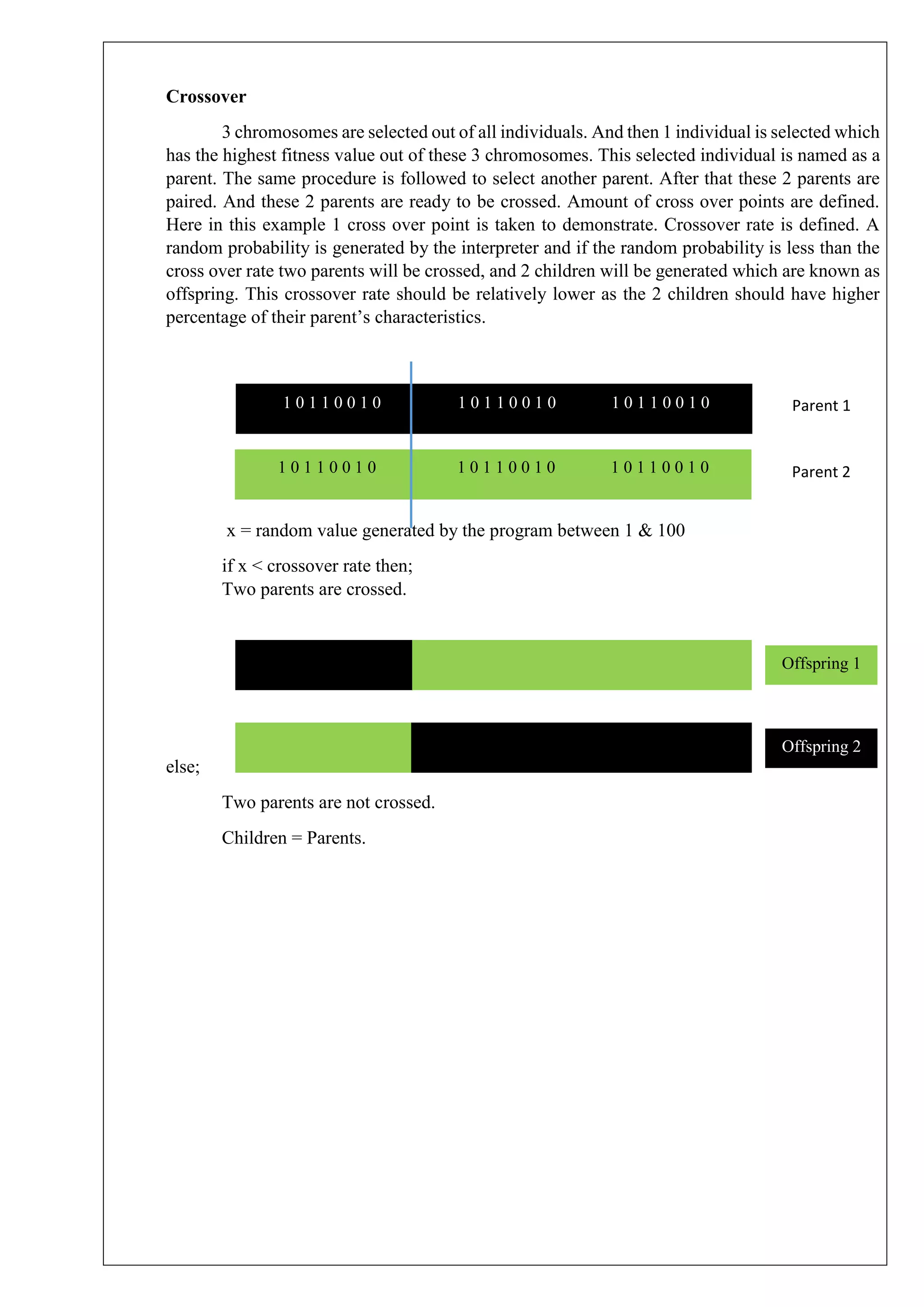
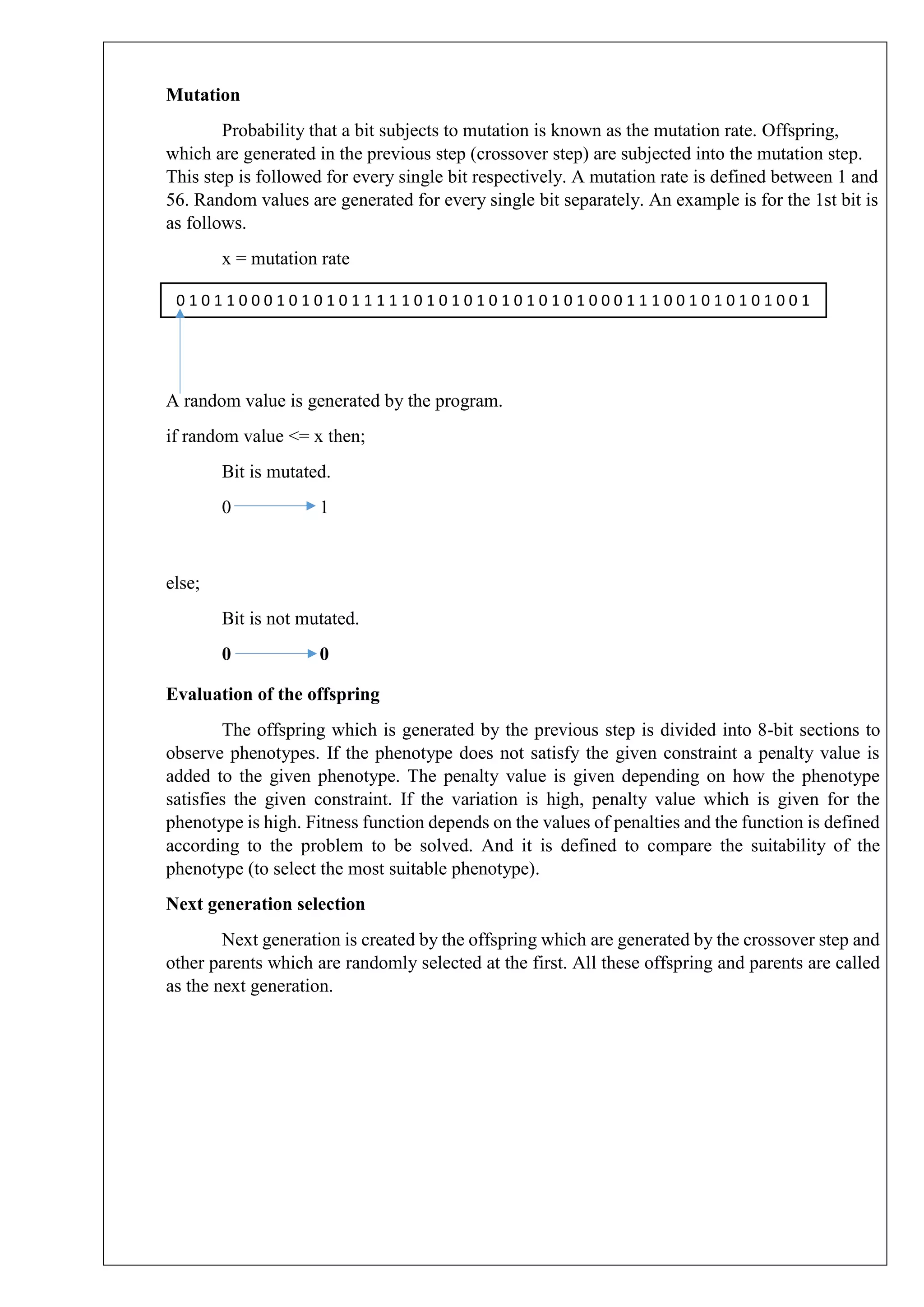
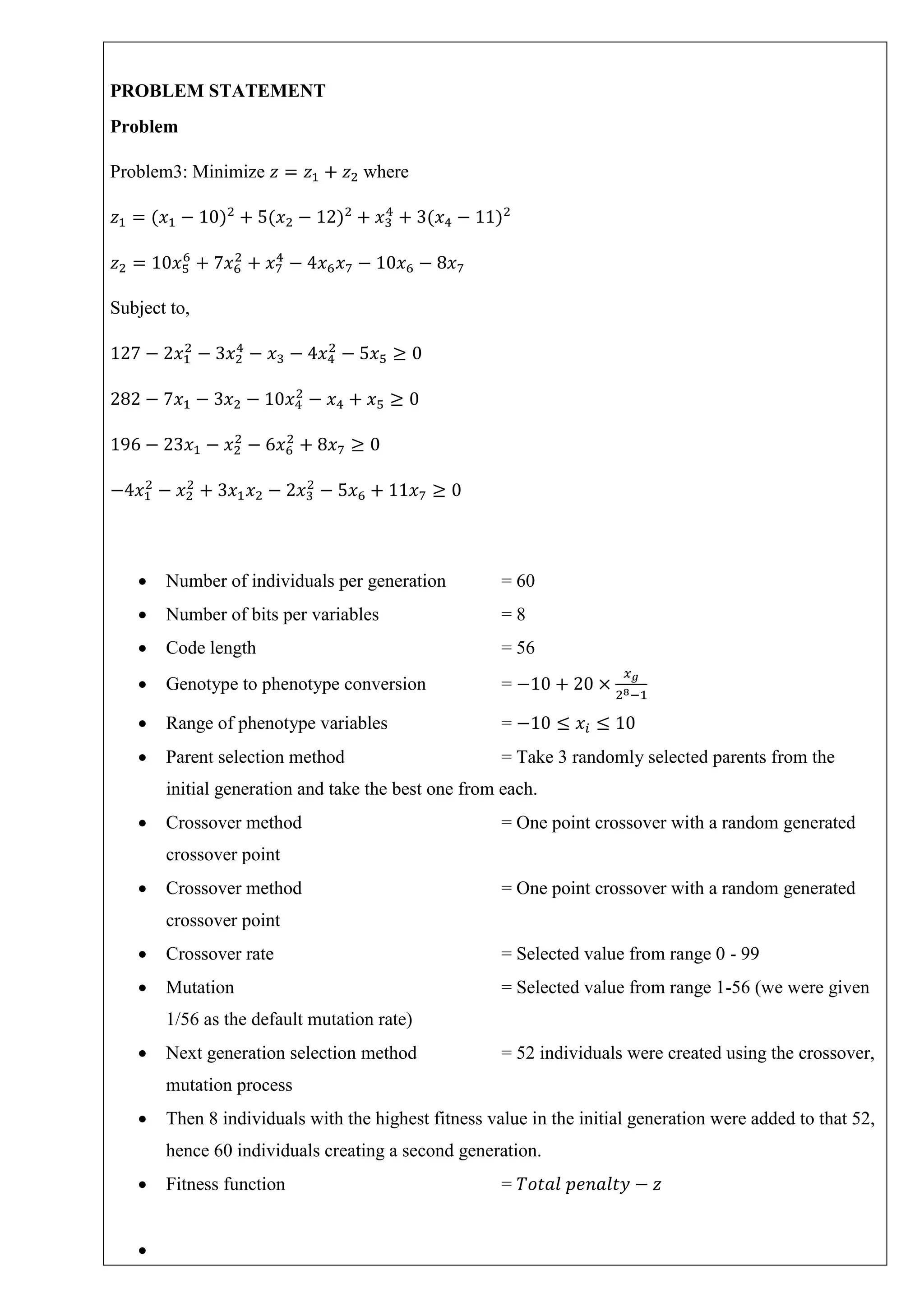
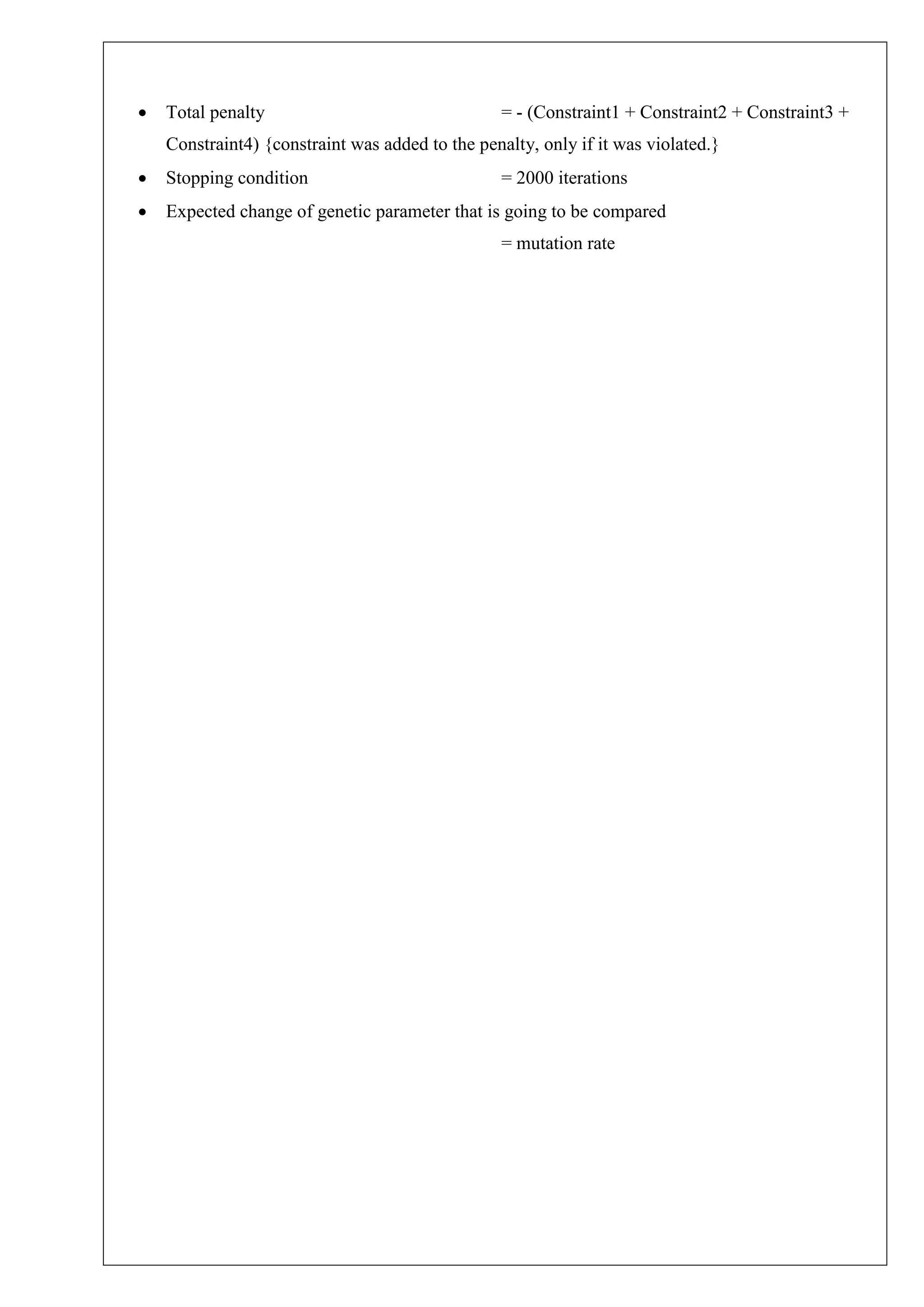
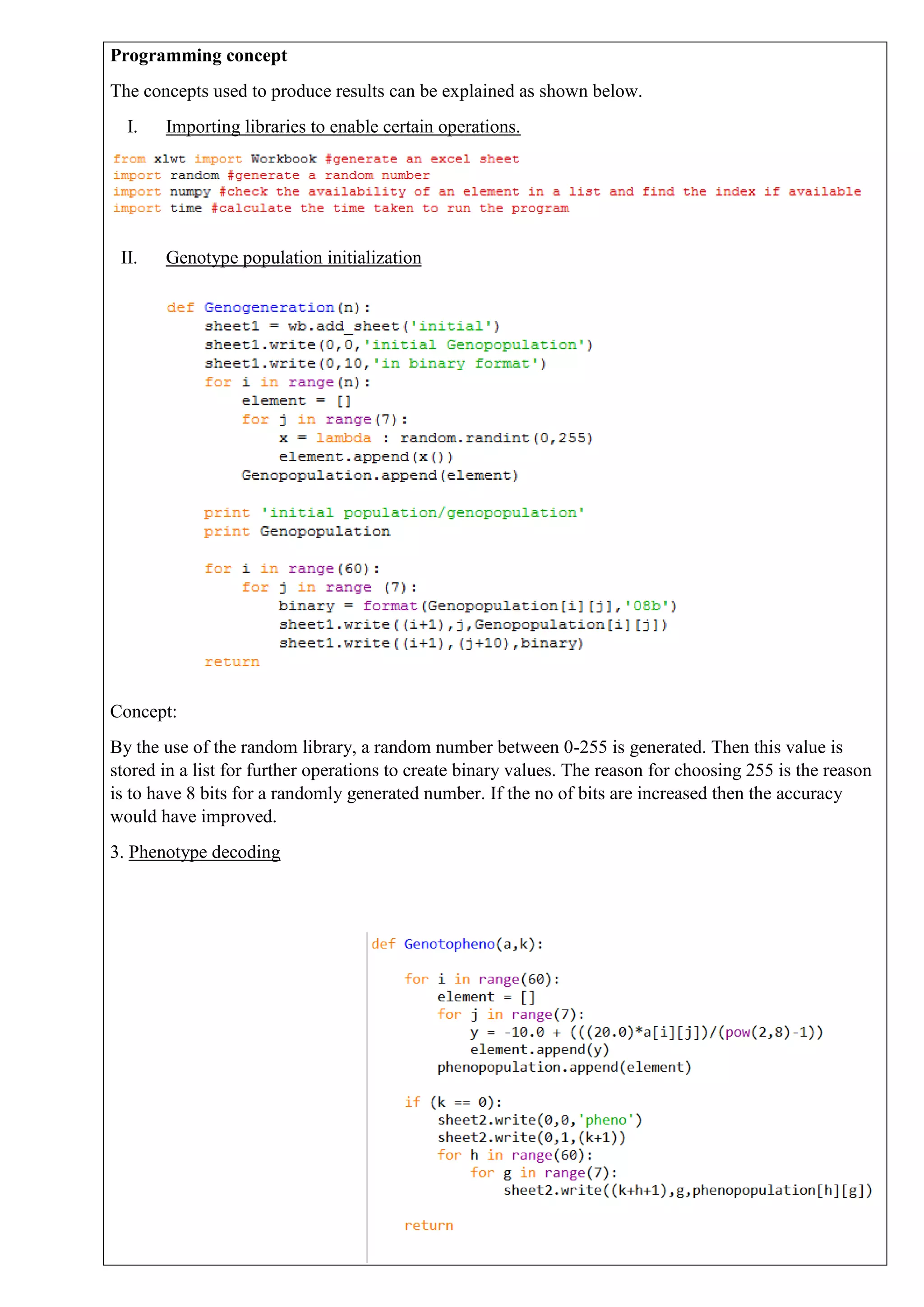
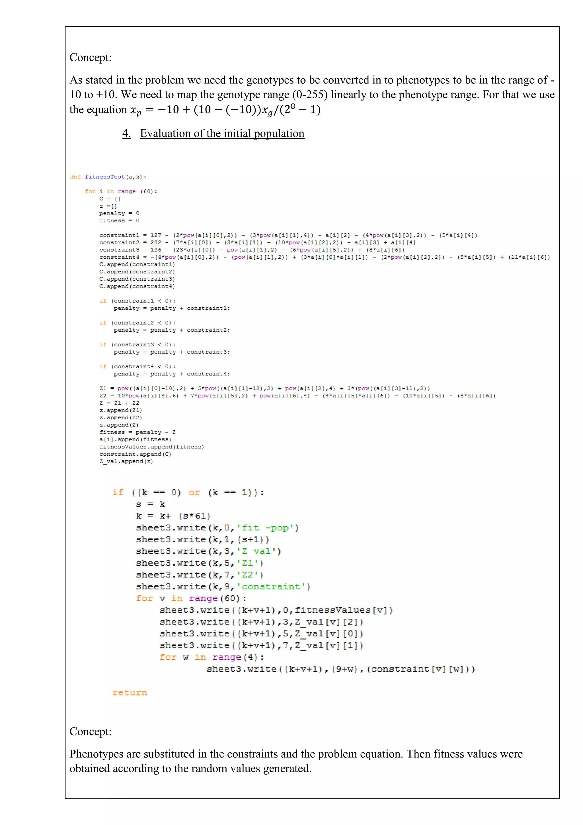
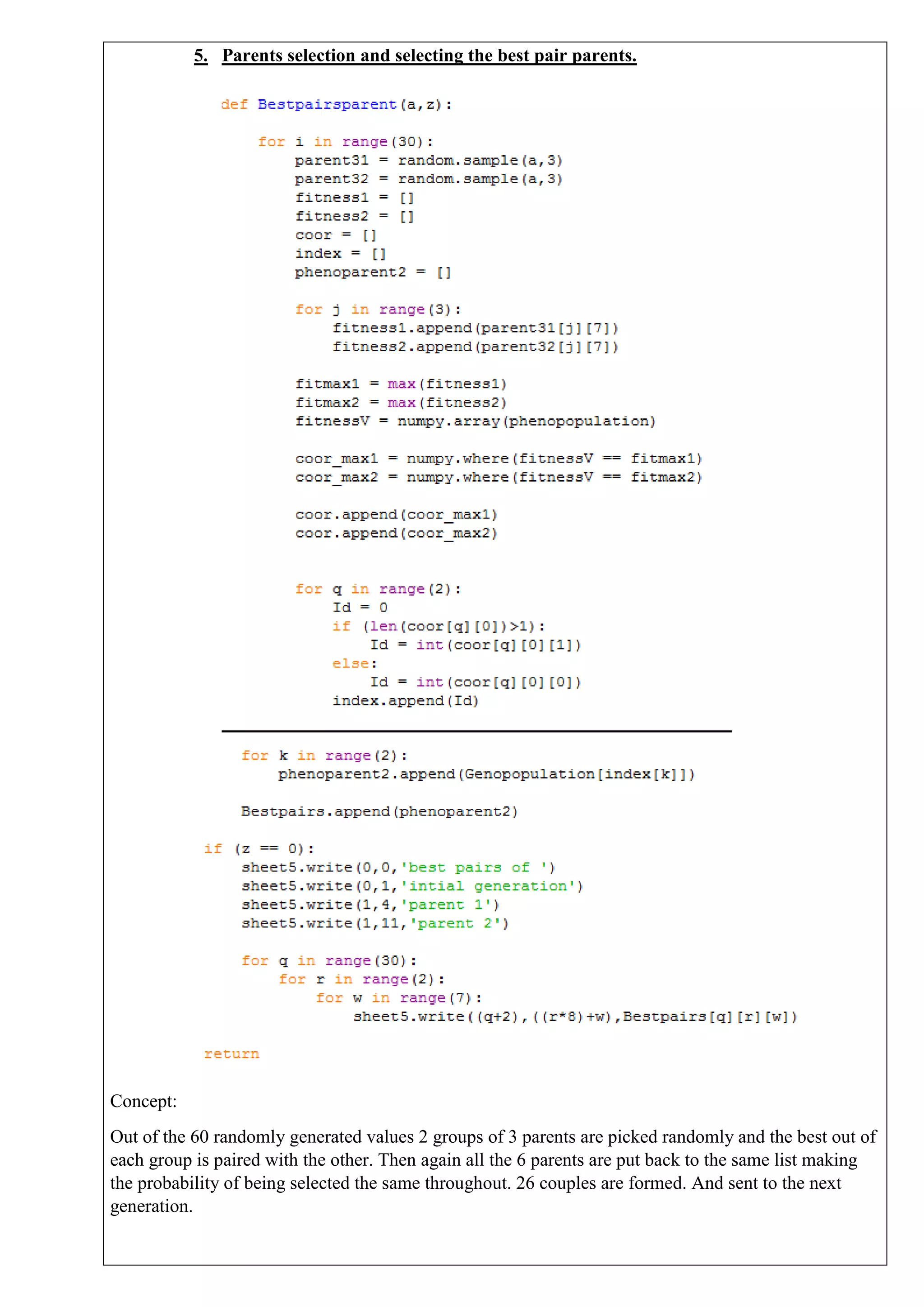
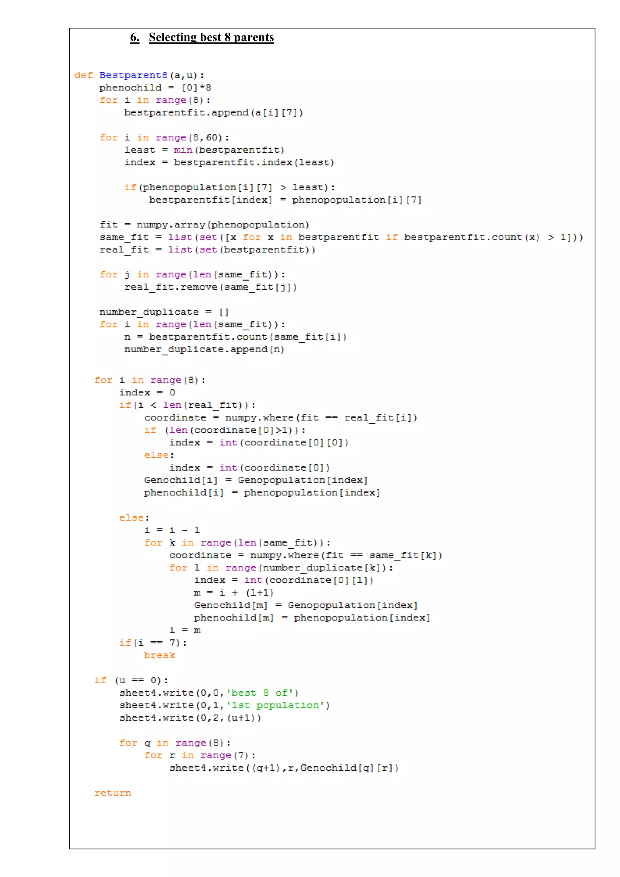
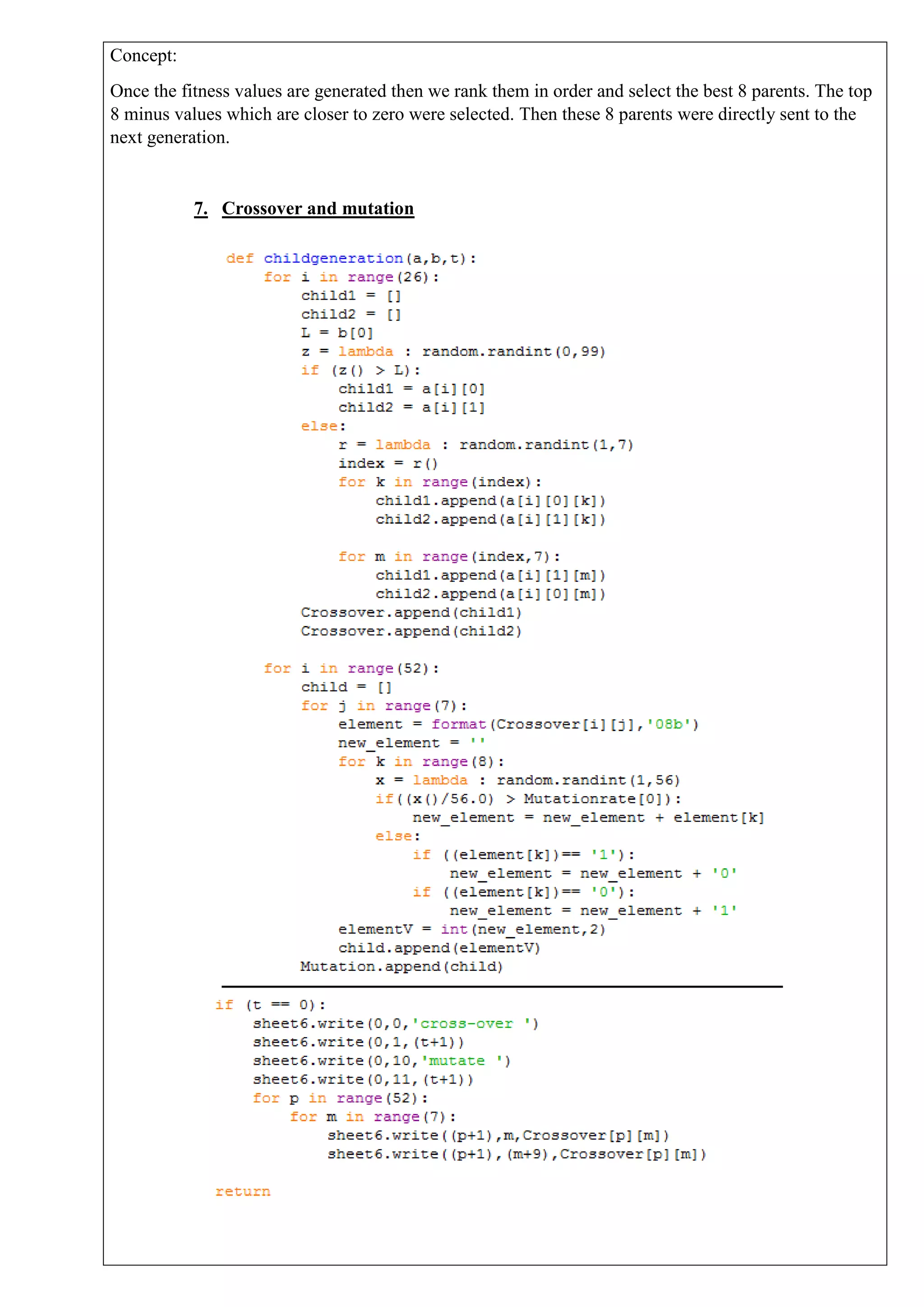
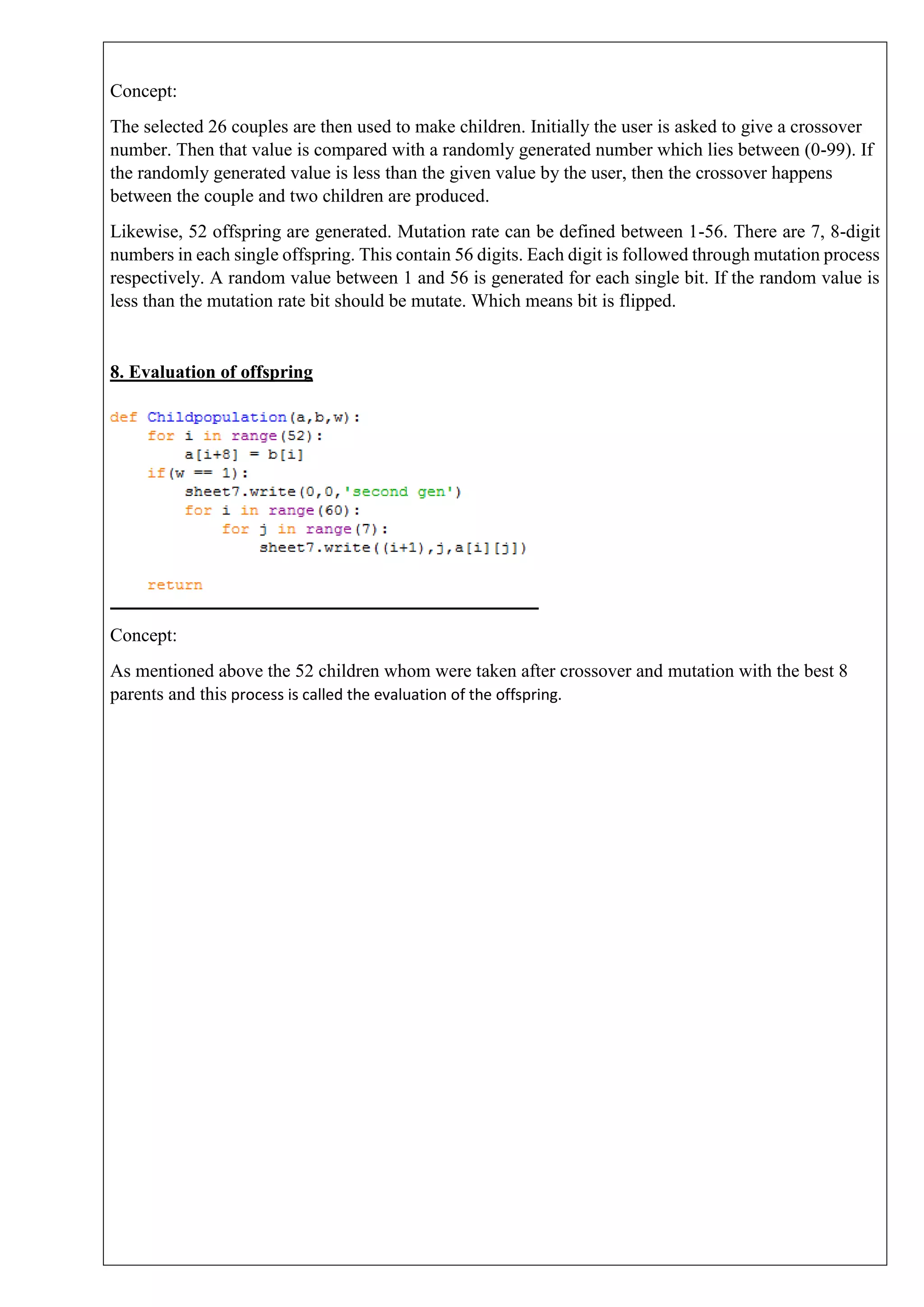
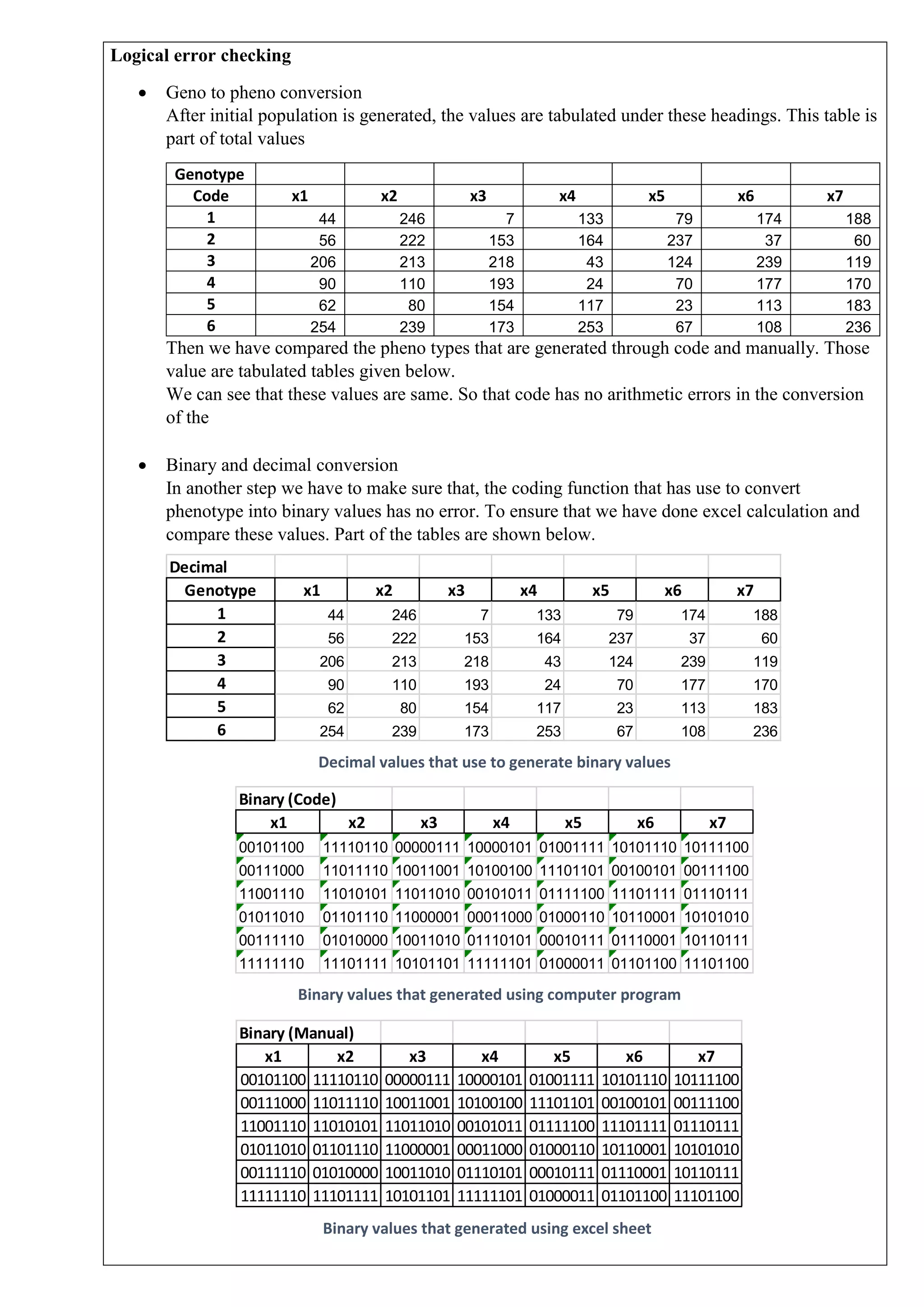
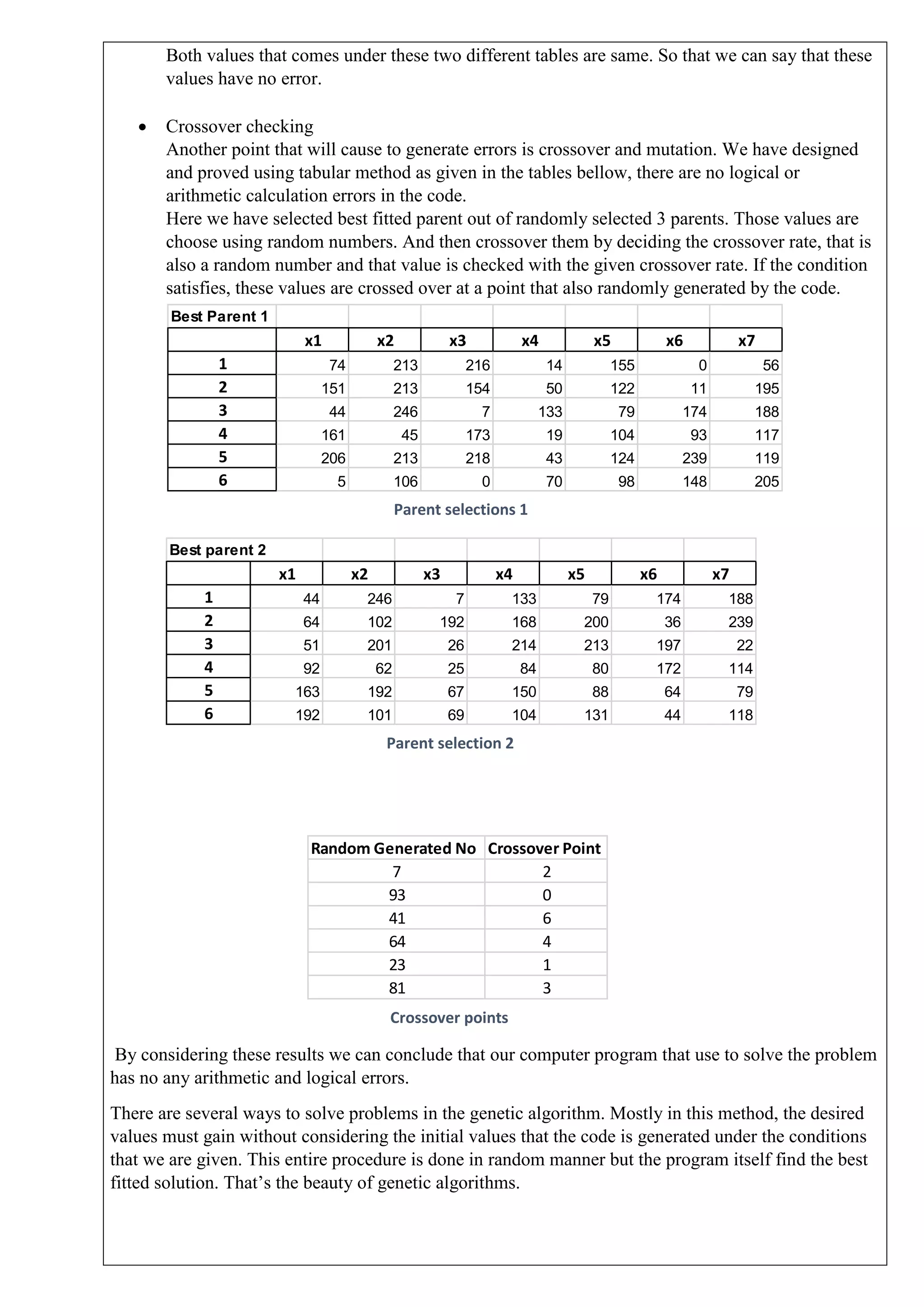
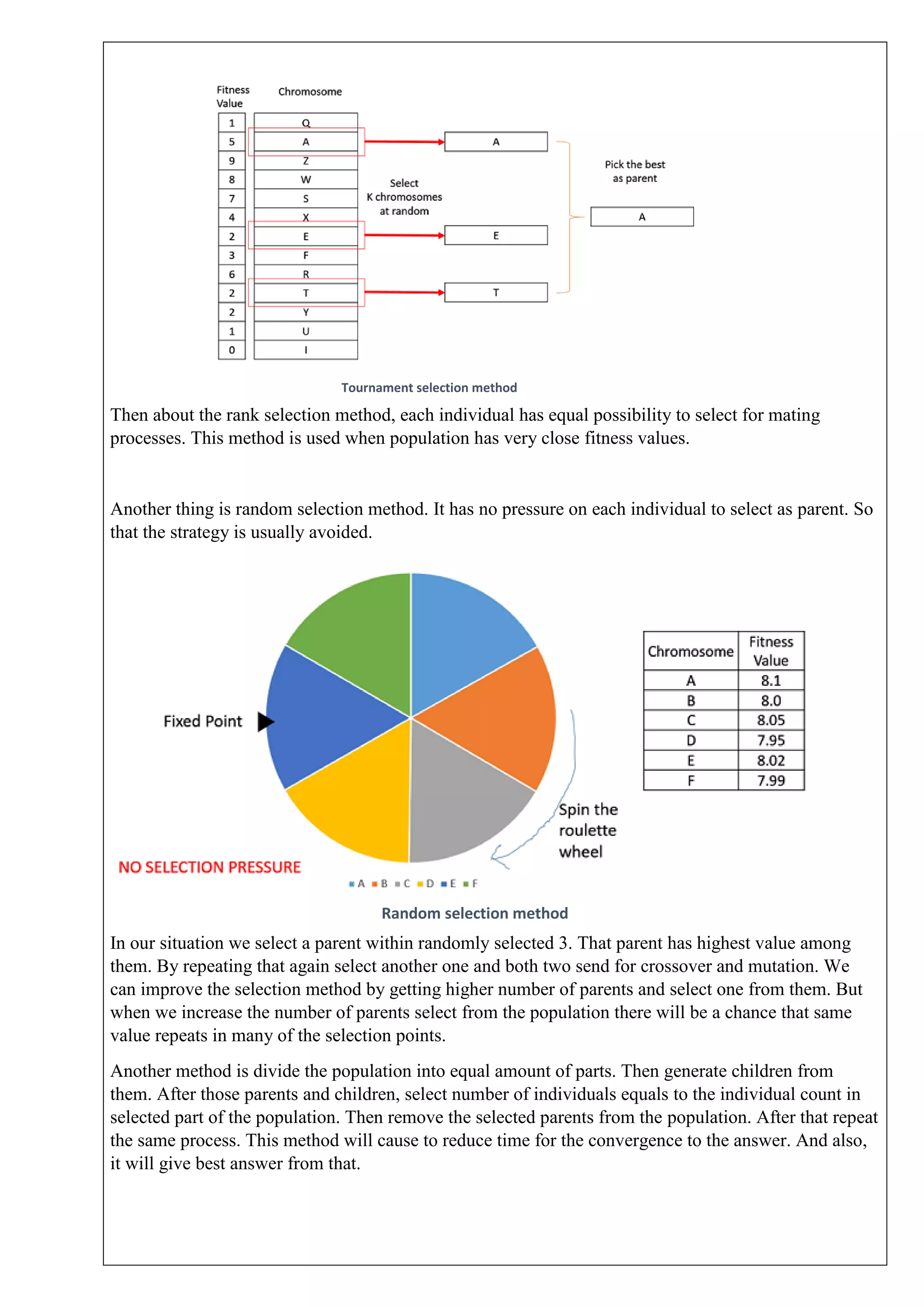
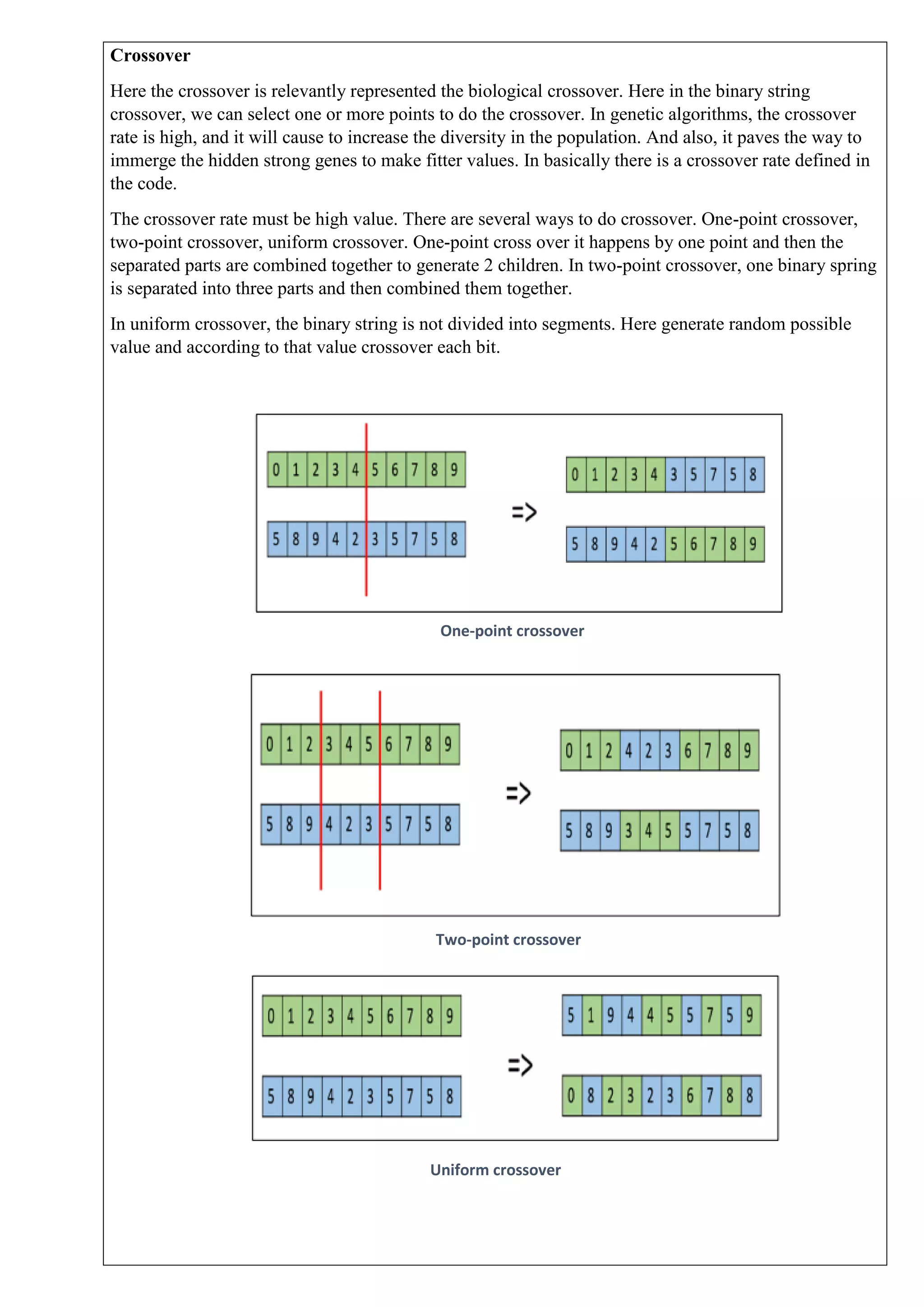
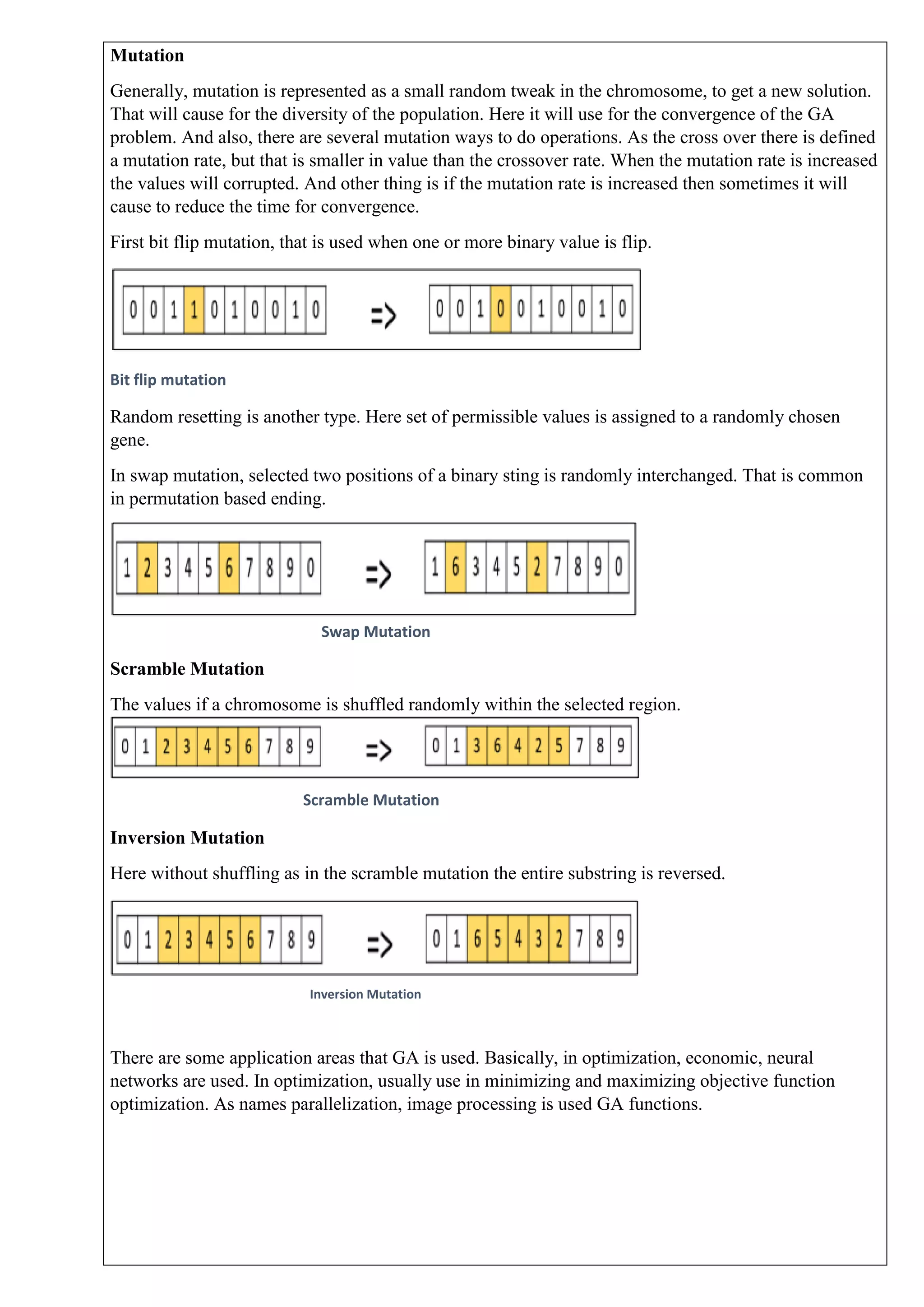
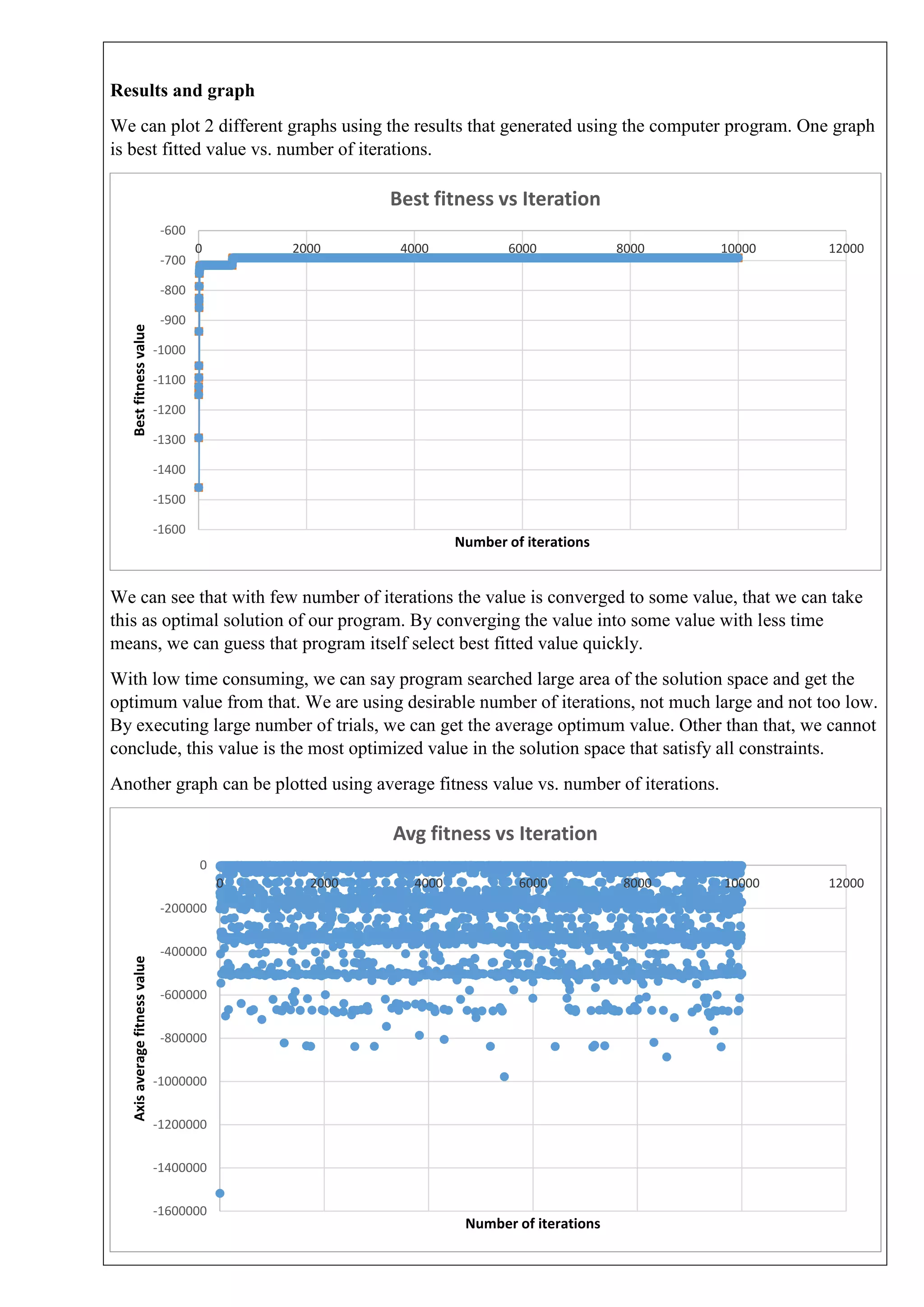
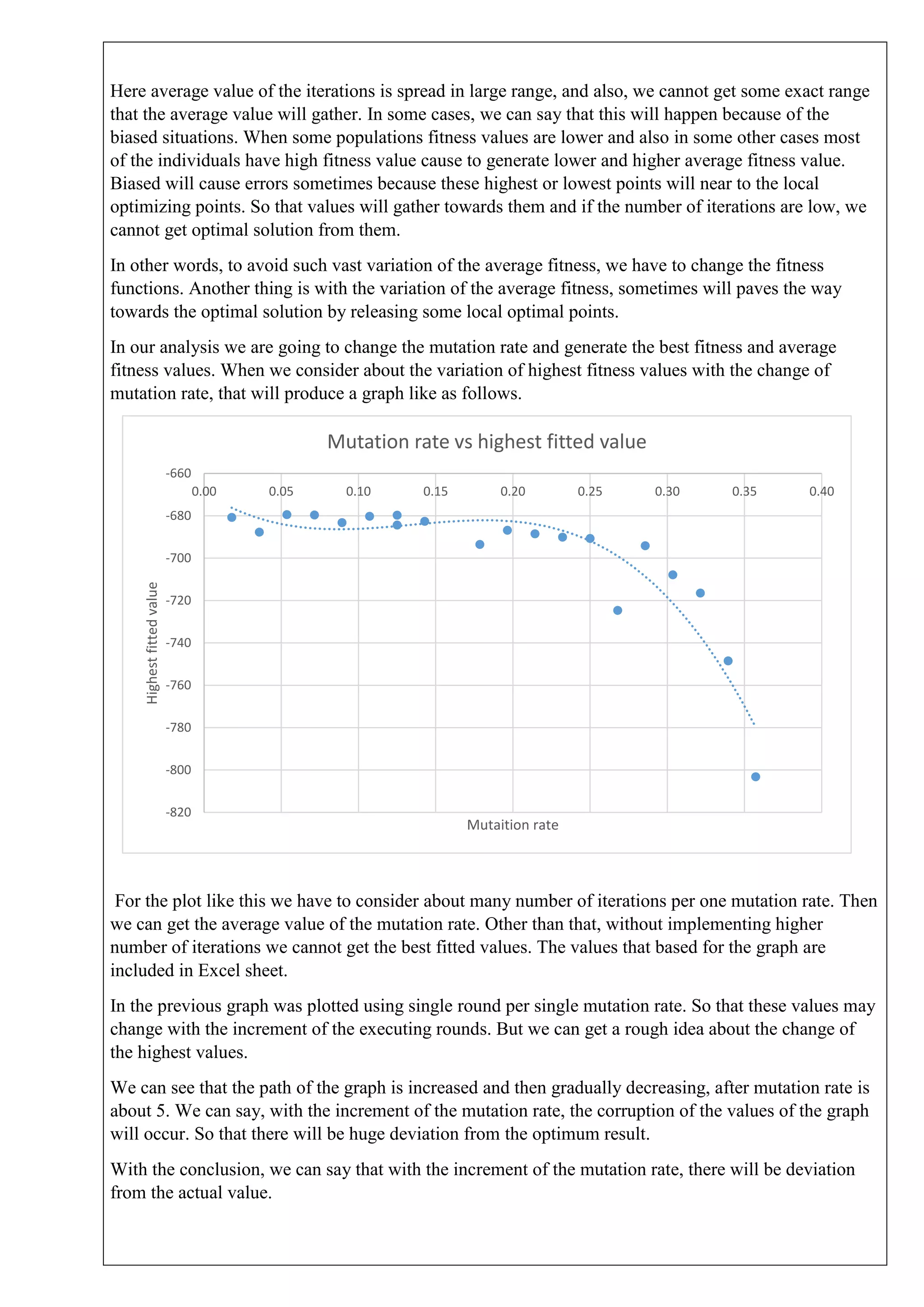
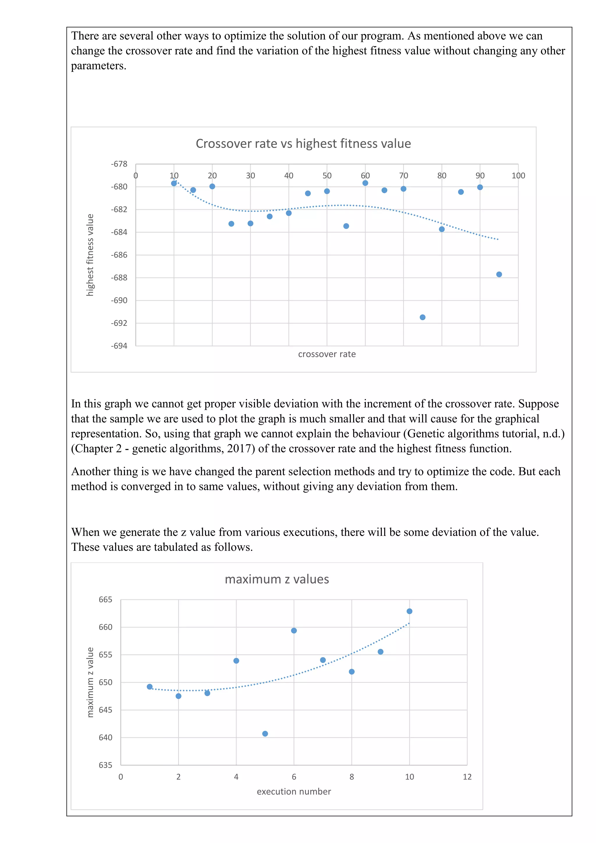
Assignment on Solving Non-Linear Programming Minimization Problem Using Genetic Algorithm NAME : Dilshan K.M.G.L. INDEX NO. : 150131A GROUP : Aeronautical I DATE OF PER. : 2017.09.29 DATE OF SUB. : 2017.10.27 GROUP MEMBERS: Abenayake D.H.S. Amarathunga H.D.V. Annasiwatta D.M. Dilanjaya H.W.S.
Abstract This report is an analysis of genetic algorithms and their applications. The concept of genetic algorithms and the evolution are being used to generate solutions in cyclic operations. We use genetic algorithm principles and functions and produce results step by step logically to find solutions to a given equation such that it satisfies given conditions. Introduction Genetic Algorithms (GAs) are based on the evolutionary ideas of natural selection and genetics. The basic techniques of the GAs are designed to simulate processes in natural systems necessary for evolution. The difference is that all individuals try to satisfy the same task and actually this is by means far simpler than actual evolution. GAs presumes that potential solution for any problem is an individual and can be represented by a set of parameters. These parameters are regarded as genes and can be represented by string values of binary form. Throughout a genetic evolution the result of the fitness function determines the quality of the solution. In genetic operation after each cycle of operation a subsequent generation is created from the current population. It is expected that from this process of evolution a better subsequent generation is created.
How to solve a genetic algorithm There is a conventional procedure which should be followed in order to solve a problem using genetic algorithms. Phenotype decoding Genotype population initialization Evaluation of the initial population Parents selection Crossover Mutation Evaluation of the off spring Next generation selection Condition Stop Start
• Genotype − Genotype is the population in the computation space. In the computation space, the solutions are represented in a way which can be easily understood and manipulated using a computing system. • Phenotype − Phenotype is the population in the actual real world solution space in which solutions are represented in a way they are represented in real world situations. 1. Genotype population initialization - genotype string is randomly generated for each individual of the generation 2. Phenotype decoding – for each individual the value regarding the actual scenario is generated for further operations. 3. Evaluation of the initial population – decoded phenotypes are used and the validity of the constraints are checked. Then depending on the satisfaction of constraints a penalty is added to the generated Z value and hence the fitness values are generated. By the obtained final value the initial population is evaluated. 4. Parents selection – once the initial population is evaluated then 3 of the elements are randomly taken and the best out of the 3 are selected. Likewise we choose another random 3 elements and the best element is chosen. Then the chosen elements are taken as parents.
Crossover 3 chromosomes are selected out of all individuals. And then 1 individual is selected which has the highest fitness value out of these 3 chromosomes. This selected individual is named as a parent. The same procedure is followed to select another parent. After that these 2 parents are paired. And these 2 parents are ready to be crossed. Amount of cross over points are defined. Here in this example 1 cross over point is taken to demonstrate. Crossover rate is defined. A random probability is generated by the interpreter and if the random probability is less than the cross over rate two parents will be crossed, and 2 children will be generated which are known as offspring. This crossover rate should be relatively lower as the 2 children should have higher percentage of their parent’s characteristics. x = random value generated by the program between 1 & 100 if x < crossover rate then; Two parents are crossed. else; Two parents are not crossed. Children = Parents. 1 0 1 1 0 0 1 0 1 0 1 1 0 0 1 0 1 0 1 1 0 0 1 0 1 0 1 1 0 0 1 0 1 0 1 1 0 0 1 0 1 0 1 1 0 0 1 0 Parent 1 Parent 2 Offspring 1 Offspring 2
Mutation Probability that a bit subjects to mutation is known as the mutation rate. Offspring, which are generated in the previous step (crossover step) are subjected into the mutation step. This step is followed for every single bit respectively. A mutation rate is defined between 1 and 56. Random values are generated for every single bit separately. An example is for the 1st bit is as follows. x = mutation rate A random value is generated by the program. if random value <= x then; Bit is mutated. 0 1 else; Bit is not mutated. 0 0 Evaluation of the offspring The offspring which is generated by the previous step is divided into 8-bit sections to observe phenotypes. If the phenotype does not satisfy the given constraint a penalty value is added to the given phenotype. The penalty value is given depending on how the phenotype satisfies the given constraint. If the variation is high, penalty value which is given for the phenotype is high. Fitness function depends on the values of penalties and the function is defined according to the problem to be solved. And it is defined to compare the suitability of the phenotype (to select the most suitable phenotype). Next generation selection Next generation is created by the offspring which are generated by the crossover step and other parents which are randomly selected at the first. All these offspring and parents are called as the next generation. 0 1 0 1 1 0 0 0 1 0 1 0 1 0 1 1 1 1 1 0 1 0 1 0 1 0 1 0 1 0 1 0 1 0 0 0 1 1 1 0 0 1 0 1 0 1 0 1 0 0 1 1
PROBLEM STATEMENT Problem Problem3: Minimize 𝑧 = 𝑧1 + 𝑧2 where 𝑧1 = (𝑥1 − 10)2 + 5(𝑥2 − 12)2 + 𝑥3 4 + 3(𝑥4 − 11)2 𝑧2 = 10𝑥5 6 + 7𝑥6 2 + 𝑥7 4 − 4𝑥6 𝑥7 − 10𝑥6 − 8𝑥7 Subject to, 127 − 2𝑥1 2 − 3𝑥2 4 − 𝑥3 − 4𝑥4 2 − 5𝑥5 ≥ 0 282 − 7𝑥1 − 3𝑥2 − 10𝑥4 2 − 𝑥4 + 𝑥5 ≥ 0 196 − 23𝑥1 − 𝑥2 2 − 6𝑥6 2 + 8𝑥7 ≥ 0 −4𝑥1 2 − 𝑥2 2 + 3𝑥1 𝑥2 − 2𝑥3 2 − 5𝑥6 + 11𝑥7 ≥ 0 • Number of individuals per generation = 60 • Number of bits per variables = 8 • Code length = 56 • Genotype to phenotype conversion = −10 + 20 × 𝑥 𝑔 28−1 • Range of phenotype variables = −10 ≤ 𝑥𝑖 ≤ 10 • Parent selection method = Take 3 randomly selected parents from the initial generation and take the best one from each. • Crossover method = One point crossover with a random generated crossover point • Crossover method = One point crossover with a random generated crossover point • Crossover rate = Selected value from range 0 - 99 • Mutation = Selected value from range 1-56 (we were given 1/56 as the default mutation rate) • Next generation selection method = 52 individuals were created using the crossover, mutation process • Then 8 individuals with the highest fitness value in the initial generation were added to that 52, hence 60 individuals creating a second generation. • Fitness function = 𝑇𝑜𝑡𝑎𝑙 𝑝𝑒𝑛𝑎𝑙𝑡𝑦 − 𝑧 •
• Total penalty = - (Constraint1 + Constraint2 + Constraint3 + Constraint4) {constraint was added to the penalty, only if it was violated.} • Stopping condition = 2000 iterations • Expected change of genetic parameter that is going to be compared = mutation rate
Programming concept The concepts used to produce results can be explained as shown below. I. Importing libraries to enable certain operations. II. Genotype population initialization Concept: By the use of the random library, a random number between 0-255 is generated. Then this value is stored in a list for further operations to create binary values. The reason for choosing 255 is the reason is to have 8 bits for a randomly generated number. If the no of bits are increased then the accuracy would have improved. 3. Phenotype decoding
Concept: As stated in the problem we need the genotypes to be converted in to phenotypes to be in the range of - 10 to +10. We need to map the genotype range (0-255) linearly to the phenotype range. For that we use the equation 𝑥 𝑝 = −10 + (10 − (−10))𝑥 𝑔/(28 − 1) 4. Evaluation of the initial population Concept: Phenotypes are substituted in the constraints and the problem equation. Then fitness values were obtained according to the random values generated.
5. Parents selection and selecting the best pair parents. Concept: Out of the 60 randomly generated values 2 groups of 3 parents are picked randomly and the best out of each group is paired with the other. Then again all the 6 parents are put back to the same list making the probability of being selected the same throughout. 26 couples are formed. And sent to the next generation.
6. Selecting best 8 parents
Concept: Once the fitness values are generated then we rank them in order and select the best 8 parents. The top 8 minus values which are closer to zero were selected. Then these 8 parents were directly sent to the next generation. 7. Crossover and mutation
Concept: The selected 26 couples are then used to make children. Initially the user is asked to give a crossover number. Then that value is compared with a randomly generated number which lies between (0-99). If the randomly generated value is less than the given value by the user, then the crossover happens between the couple and two children are produced. Likewise, 52 offspring are generated. Mutation rate can be defined between 1-56. There are 7, 8-digit numbers in each single offspring. This contain 56 digits. Each digit is followed through mutation process respectively. A random value between 1 and 56 is generated for each single bit. If the random value is less than the mutation rate bit should be mutate. Which means bit is flipped. 8. Evaluation of offspring Concept: As mentioned above the 52 children whom were taken after crossover and mutation with the best 8 parents and this process is called the evaluation of the offspring.
Logical error checking • Geno to pheno conversion After initial population is generated, the values are tabulated under these headings. This table is part of total values Genotype Code x1 x2 x3 x4 x5 x6 x7 1 44 246 7 133 79 174 188 2 56 222 153 164 237 37 60 3 206 213 218 43 124 239 119 4 90 110 193 24 70 177 170 5 62 80 154 117 23 113 183 6 254 239 173 253 67 108 236 Then we have compared the pheno types that are generated through code and manually. Those value are tabulated tables given below. We can see that these values are same. So that code has no arithmetic errors in the conversion of the • Binary and decimal conversion In another step we have to make sure that, the coding function that has use to convert phenotype into binary values has no error. To ensure that we have done excel calculation and compare these values. Part of the tables are shown below. Decimal Genotype x1 x2 x3 x4 x5 x6 x7 1 44 246 7 133 79 174 188 2 56 222 153 164 237 37 60 3 206 213 218 43 124 239 119 4 90 110 193 24 70 177 170 5 62 80 154 117 23 113 183 6 254 239 173 253 67 108 236 Decimal values that use to generate binary values Binary (Code) x1 x2 x3 x4 x5 x6 x7 00101100 11110110 00000111 10000101 01001111 10101110 10111100 00111000 11011110 10011001 10100100 11101101 00100101 00111100 11001110 11010101 11011010 00101011 01111100 11101111 01110111 01011010 01101110 11000001 00011000 01000110 10110001 10101010 00111110 01010000 10011010 01110101 00010111 01110001 10110111 11111110 11101111 10101101 11111101 01000011 01101100 11101100 Binary values that generated using computer program Binary (Manual) x1 x2 x3 x4 x5 x6 x7 00101100 11110110 00000111 10000101 01001111 10101110 10111100 00111000 11011110 10011001 10100100 11101101 00100101 00111100 11001110 11010101 11011010 00101011 01111100 11101111 01110111 01011010 01101110 11000001 00011000 01000110 10110001 10101010 00111110 01010000 10011010 01110101 00010111 01110001 10110111 11111110 11101111 10101101 11111101 01000011 01101100 11101100 Binary values that generated using excel sheet
Both values that comes under these two different tables are same. So that we can say that these values have no error. • Crossover checking Another point that will cause to generate errors is crossover and mutation. We have designed and proved using tabular method as given in the tables bellow, there are no logical or arithmetic calculation errors in the code. Here we have selected best fitted parent out of randomly selected 3 parents. Those values are choose using random numbers. And then crossover them by deciding the crossover rate, that is also a random number and that value is checked with the given crossover rate. If the condition satisfies, these values are crossed over at a point that also randomly generated by the code. By considering these results we can conclude that our computer program that use to solve the problem has no any arithmetic and logical errors. There are several ways to solve problems in the genetic algorithm. Mostly in this method, the desired values must gain without considering the initial values that the code is generated under the conditions that we are given. This entire procedure is done in random manner but the program itself find the best fitted solution. That’s the beauty of genetic algorithms. Best Parent 1 x1 x2 x3 x4 x5 x6 x7 1 74 213 216 14 155 0 56 2 151 213 154 50 122 11 195 3 44 246 7 133 79 174 188 4 161 45 173 19 104 93 117 5 206 213 218 43 124 239 119 6 5 106 0 70 98 148 205 Parent selections 1 Best parent 2 x1 x2 x3 x4 x5 x6 x7 1 44 246 7 133 79 174 188 2 64 102 192 168 200 36 239 3 51 201 26 214 213 197 22 4 92 62 25 84 80 172 114 5 163 192 67 150 88 64 79 6 192 101 69 104 131 44 118 Parent selection 2 Random Generated No Crossover Point 7 2 93 0 41 6 64 4 23 1 81 3 Crossover points
Phenotype Codex1x2x3x4x5x6x7z1z2z1234Fitness 1-6.549029.294118-9.450980.431373-3.803923.6470594.7450988623.81330752.739376.52-22315.9-597.485218.4014-585.223-62875.1 2-5.607847.41176522.8627458.588235-7.09804-5.29412563.50940136804014244-9066.94264.7451-74.5998-336.163-4023722 36.1568636.7058827.098039-6.62745-0.274518.745098-0.666673625.451476.74164102.193-6196.83-278.684-454.77-224.558-11257 4-2.94118-1.372555.137255-8.11765-4.50983.8823533.3333332854.55884240.7687095.31-147.12146.39985197.9938-59.9031-87302.3 5-5.13725-3.725492.078431-0.82353-8.19608-1.137254.3529411903.64130317183033622-467.497278.5659327.341-17.0996-3034107 69.9215698.7450983.5686279.843137-4.7451-1.529418.509804219.1759119408.6119627.8-17983.344.37447-54.629-134.147-137800 Constraints/Penalties Codegeneratedphenotypevalues Phenotype Manualx1x2x3x4x5x6x7z1z2z1234Fitness 1-6.549029.294118-9.450980.431373-3.803923.6470594.7450988623.81330752.739376.52-22315.889-597.48481218.4013841-585.22261-62875.1 2-5.6078437.41176522.8627458.588235-7.09804-5.29412563.50940136804014244-9066.9357264.745098-74.59976932-336.16301-4023722 36.15686276.7058827.098039-6.62745-0.274518.745098-0.666673625.451476.74164102.193-6196.8264-278.68435-454.7704729-224.55825-11257 4-2.941176-1.372555.137255-8.11765-4.50983.8823533.3333332854.55884240.7687095.31-147.1211846.3998462197.9938485-59.903114-87302.3 5-5.137255-3.725492.078431-0.82353-8.19608-1.137254.3529411903.64130317183033622-467.49662278.565936327.3410227-17.099577-3034107 69.92156868.7450983.5686279.843137-4.7451-1.529418.509804219.1759119408.6119627.8-17983.34344.3744714-54.62898885-134.14687-137800 Constraints/Penalties Manuallycalculatedphenotypevalues AfterCrossover(Offspring1)Offspring(Offspring2) x1x2x3x4x5x6x7x1x2x3x4x5x6x7 17421371337917418814424621614155056 2151213154501221119526410219216820036239 3442467133791742235120126214213197188 416145173198017211449262258410493117 520619267150886479516321321843124239119 651060104131441186192101697098148205 Manuallycalculatedmutations
The main idea of the population is come from simply as subset of solution space. Also, we can say that chromosomes. In a population there must be diversity, in initial condition. But after some iterations all the population will have same value, but it is not a compulsory condition. And also, when we select large number of population for the calculation, that will cause to slow down the converging process. And on the other hand, when we select small number of individuals as population, the diversity of the population is not keep. Other than that, it will not produce good mating pool for generate new population. Genotype population initialization According to the problem that we have to solve using GA, we have to pay our attention to 7 variables and 4 constraints. First of all, we have to get initial phenotype from the code. Instead of randomly select genotype, we can manually enter genotypes (heuristic initialization). These are two different methods. We cannot say directly what is the most efficient way among these two. To get clear picture of the efficiency of the method, we have to run the code under both of these methods and get series of solutions. That may pave the way to get somewhat clear understanding about the efficiency of each method. And also, there are some ways for population models called steady state model and generational model. In steady state model, generate 2 off springs in each iteration and those off-springs replace one or two individuals from the population. So that the population is constant and the change is continuous. In generational method we generate some offspring equal to the new population number. That method is used during the iterations. Basically, we can use combination of both those methods to generate new population. Phenotype decoding – mapping genotype to phenotype When we consider about the phenotype decoding, that means we are going to map the values that generated by the code itself. The aim is to set the variable values that suitable for the range that we are trying get. The range is different from problem to problem, because of the type and conditions of the problem. We can select different mapping functions according to the problem. We can use linear mapping functions, polynomial mapping functions, logarithmic mapping functions, exponential mapping functions etc. When we are considering about the bias, we have to avoid linear mapping function. In linear mapping function there is no special conditions that avoid biasing to highest values or lowest values. When we consider about the biasing there will be some values that generated are biased to highest values of the inequality. On the other hand, these values can be gathered into lower value. In some researchers we have seen that these types of values will get higher time to converge into the desired value. And also, these values will get lower fitness with compared to the non-biased mapping values. When we think about the mapping values that not much close to the higher merging as well as lower merging. Then we have to define definitely nonlinear function to get the values. We can use parabolic shape function when we have to avoid biasing to the lowest possible values. When we use hyperbolic function that mapping function will have completely different. So that we have to select best fitting mapping function. In same problem there will be several mapping functions. In most problems, there is a range for each parameter in a problem. Otherwise we have to introduce a range of possible values that the parameter can get. In multi variable problem, we can introduce unique mapping function for each variable in order to avoid some undesirable values or to reduce the probability to generate such values. In GA basically use randomness. So that we have to reduce the probability that these biased values or undesirable values are generated.
Evaluation of initial population In initial generation there are no crossover or mutation. That is purely based on the values that the code is generated and the mapping function we are used. After generating initial population, we have to get the idea of the fitness value of each individual have. So that we are going to define fitness function. This fitness function is a representation of a deviation from the most optimized value and the value generated from the code. Fitness function is the most crucial function that used in GA. We say that because the optimum value that we can get from the code is based on out fitness function. To calculate the fitness there are some methods. Basically, programmer has to decide the function that he is going to use to optimize the solutions. To get the variation from the actual value we introduce penalty value if the variables are violated the constraints. These penalty values decide the eligibility of the variable. As an instance, when we think about problem that has four constraints, we can introduce 4 penalty values, one for each. And in simple way to optimize the fitness, the sum of the penalty values can be adding or subtract from the final optimized value. That will help to select the next generation process to decide the fitness of each individual. Some of the cases the fitness function can be used as the objective function. but when we consider about the nonlinear more complex problems cannot use the objective function as same as this. Basically, fitness function should have fast computing method. Because slow computation of the fitness value can be affect to slow the converting process. Parent selection methods After generating and evaluating initial population we have to mate selected parents to generate new population. There are several ways of selecting parents, and we have to choose one of them for our analysis. As we can see that parent selection method is very crucial because that will affect directly for the fitter solution and time to converge. And also, these parent selection methods don’t use only “best” fittest parents for the next solution. Main reason is we cannot neglect all low fitted phenotypes without selecting them for the mutation or crossover. That will cause for reduce diversity of the population. There will be good genes, proper genes in worst individuals and sometimes these best genes will immerge through crossover and mutation in another population. So that maintaining good diversity in the population in extremely crucial for the success of a GA. After sometimes population is converged to some premature convergence and is an undesirable condition in a GA. That will be the optimum solution. Basically, the aim of parent selection is to select two individuals from the existing pool of individuals and use to mate and recombine to create off-springs to next generation. Most popular method is select parents according to the fitness value of them. According to that method each individual has a probability values to select for the next generation. So that fitter solutions have higher chances to participate for the mating purpose. There are several selection methods. Roulette wheel selection method, Stochastic universal Sampling method, tournament selection method, rank selection method, random selection method. In roulette wheel selection method, the fitness value of the individuals is represented by the area of a circle. Higher the fines value, higher they are represented in the circle, higher chance to select to next generation. These values are generated by dividing the value of fitness, total sum of fitness.
In stochastic universal sampling, both parents that use to crossover are selected at the same time. Simply these values are at the opposite side of the circle. There will be a problem with the fitness proportionate methods will not work when the fitness values get negative. When we consider about the tournament selection method, basically randomly selected parents are shifted to mating process and produce children. In literature this will work even for negative fitness values. Here select 2 or more chromosomes from the pool and among them select best chromosome. In the second stage, repeat the process and get another chromosome until select best fit one. This method usually uses when there are higher number of individuals in a population. Stochastic universal sampling Roulette wheel selection method
Then about the rank selection method, each individual has equal possibility to select for mating processes. This method is used when population has very close fitness values. Another thing is random selection method. It has no pressure on each individual to select as parent. So that the strategy is usually avoided. In our situation we select a parent within randomly selected 3. That parent has highest value among them. By repeating that again select another one and both two send for crossover and mutation. We can improve the selection method by getting higher number of parents and select one from them. But when we increase the number of parents select from the population there will be a chance that same value repeats in many of the selection points. Another method is divide the population into equal amount of parts. Then generate children from them. After those parents and children, select number of individuals equals to the individual count in selected part of the population. Then remove the selected parents from the population. After that repeat the same process. This method will cause to reduce time for the convergence to the answer. And also, it will give best answer from that. Tournament selection method Random selection method
Crossover Here the crossover is relevantly represented the biological crossover. Here in the binary string crossover, we can select one or more points to do the crossover. In genetic algorithms, the crossover rate is high, and it will cause to increase the diversity in the population. And also, it paves the way to immerge the hidden strong genes to make fitter values. In basically there is a crossover rate defined in the code. The crossover rate must be high value. There are several ways to do crossover. One-point crossover, two-point crossover, uniform crossover. One-point cross over it happens by one point and then the separated parts are combined together to generate 2 children. In two-point crossover, one binary spring is separated into three parts and then combined them together. In uniform crossover, the binary string is not divided into segments. Here generate random possible value and according to that value crossover each bit. One-point crossover Two-point crossover Uniform crossover
Mutation Generally, mutation is represented as a small random tweak in the chromosome, to get a new solution. That will cause for the diversity of the population. Here it will use for the convergence of the GA problem. And also, there are several mutation ways to do operations. As the cross over there is defined a mutation rate, but that is smaller in value than the crossover rate. When the mutation rate is increased the values will corrupted. And other thing is if the mutation rate is increased then sometimes it will cause to reduce the time for convergence. First bit flip mutation, that is used when one or more binary value is flip. Bit flip mutation Random resetting is another type. Here set of permissible values is assigned to a randomly chosen gene. In swap mutation, selected two positions of a binary sting is randomly interchanged. That is common in permutation based ending. Scramble Mutation The values if a chromosome is shuffled randomly within the selected region. Inversion Mutation Here without shuffling as in the scramble mutation the entire substring is reversed. There are some application areas that GA is used. Basically, in optimization, economic, neural networks are used. In optimization, usually use in minimizing and maximizing objective function optimization. As names parallelization, image processing is used GA functions. Swap Mutation Scramble Mutation Inversion Mutation
Results and graph We can plot 2 different graphs using the results that generated using the computer program. One graph is best fitted value vs. number of iterations. We can see that with few number of iterations the value is converged to some value, that we can take this as optimal solution of our program. By converging the value into some value with less time means, we can guess that program itself select best fitted value quickly. With low time consuming, we can say program searched large area of the solution space and get the optimum value from that. We are using desirable number of iterations, not much large and not too low. By executing large number of trials, we can get the average optimum value. Other than that, we cannot conclude, this value is the most optimized value in the solution space that satisfy all constraints. Another graph can be plotted using average fitness value vs. number of iterations. -1600 -1500 -1400 -1300 -1200 -1100 -1000 -900 -800 -700 -600 0 2000 4000 6000 8000 10000 12000 Bestfitnessvalue Number of iterations Best fitness vs Iteration -1600000 -1400000 -1200000 -1000000 -800000 -600000 -400000 -200000 0 0 2000 4000 6000 8000 10000 12000 Axisaveragefitnessvalue Number of iterations Avg fitness vs Iteration
Here average value of the iterations is spread in large range, and also, we cannot get some exact range that the average value will gather. In some cases, we can say that this will happen because of the biased situations. When some populations fitness values are lower and also in some other cases most of the individuals have high fitness value cause to generate lower and higher average fitness value. Biased will cause errors sometimes because these highest or lowest points will near to the local optimizing points. So that values will gather towards them and if the number of iterations are low, we cannot get optimal solution from them. In other words, to avoid such vast variation of the average fitness, we have to change the fitness functions. Another thing is with the variation of the average fitness, sometimes will paves the way towards the optimal solution by releasing some local optimal points. In our analysis we are going to change the mutation rate and generate the best fitness and average fitness values. When we consider about the variation of highest fitness values with the change of mutation rate, that will produce a graph like as follows. For the plot like this we have to consider about many number of iterations per one mutation rate. Then we can get the average value of the mutation rate. Other than that, without implementing higher number of iterations we cannot get the best fitted values. The values that based for the graph are included in Excel sheet. In the previous graph was plotted using single round per single mutation rate. So that these values may change with the increment of the executing rounds. But we can get a rough idea about the change of the highest values. We can see that the path of the graph is increased and then gradually decreasing, after mutation rate is about 5. We can say, with the increment of the mutation rate, the corruption of the values of the graph will occur. So that there will be huge deviation from the optimum result. With the conclusion, we can say that with the increment of the mutation rate, there will be deviation from the actual value. -820 -800 -780 -760 -740 -720 -700 -680 -660 0.00 0.05 0.10 0.15 0.20 0.25 0.30 0.35 0.40 Highestfittedvalue Mutaition rate Mutation rate vs highest fitted value
There are several other ways to optimize the solution of our program. As mentioned above we can change the crossover rate and find the variation of the highest fitness value without changing any other parameters. In this graph we cannot get proper visible deviation with the increment of the crossover rate. Suppose that the sample we are used to plot the graph is much smaller and that will cause for the graphical representation. So, using that graph we cannot explain the behaviour (Genetic algorithms tutorial, n.d.) (Chapter 2 - genetic algorithms, 2017) of the crossover rate and the highest fitness function. Another thing is we have changed the parent selection methods and try to optimize the code. But each method is converged in to same values, without giving any deviation from them. When we generate the z value from various executions, there will be some deviation of the value. These values are tabulated as follows. 635 640 645 650 655 660 665 0 2 4 6 8 10 12 maximumzvalue execution number maximum z values -694 -692 -690 -688 -686 -684 -682 -680 -678 0 10 20 30 40 50 60 70 80 90 100 highestfitnessvalue crossover rate Crossover rate vs highest fitness value
References Chapter 2 - genetic algorithms. (2017). In Kramer. Springer. Genetic algorithms tutorial. (n.d.). Results and work conducted Index No Name Work 150023U H.D.V Amarathunga Coding 150131A K.M.G.L Dilshan Manual checking 150127R H.W.S Dilanjaya Manual checking 150031R D.M Annasiwatta Report Editing 150008E D.H.S Abenayake Report Editing

Solving non linear programming minimization problem using genetic algorithm

  • 1.
    Assignment on SolvingNon-Linear Programming Minimization Problem Using Genetic Algorithm NAME : Dilshan K.M.G.L. INDEX NO. : 150131A GROUP : Aeronautical I DATE OF PER. : 2017.09.29 DATE OF SUB. : 2017.10.27 GROUP MEMBERS: Abenayake D.H.S. Amarathunga H.D.V. Annasiwatta D.M. Dilanjaya H.W.S.
  • 2.
    Abstract This report isan analysis of genetic algorithms and their applications. The concept of genetic algorithms and the evolution are being used to generate solutions in cyclic operations. We use genetic algorithm principles and functions and produce results step by step logically to find solutions to a given equation such that it satisfies given conditions. Introduction Genetic Algorithms (GAs) are based on the evolutionary ideas of natural selection and genetics. The basic techniques of the GAs are designed to simulate processes in natural systems necessary for evolution. The difference is that all individuals try to satisfy the same task and actually this is by means far simpler than actual evolution. GAs presumes that potential solution for any problem is an individual and can be represented by a set of parameters. These parameters are regarded as genes and can be represented by string values of binary form. Throughout a genetic evolution the result of the fitness function determines the quality of the solution. In genetic operation after each cycle of operation a subsequent generation is created from the current population. It is expected that from this process of evolution a better subsequent generation is created.
  • 3.
    How to solvea genetic algorithm There is a conventional procedure which should be followed in order to solve a problem using genetic algorithms. Phenotype decoding Genotype population initialization Evaluation of the initial population Parents selection Crossover Mutation Evaluation of the off spring Next generation selection Condition Stop Start
  • 4.
    • Genotype −Genotype is the population in the computation space. In the computation space, the solutions are represented in a way which can be easily understood and manipulated using a computing system. • Phenotype − Phenotype is the population in the actual real world solution space in which solutions are represented in a way they are represented in real world situations. 1. Genotype population initialization - genotype string is randomly generated for each individual of the generation 2. Phenotype decoding – for each individual the value regarding the actual scenario is generated for further operations. 3. Evaluation of the initial population – decoded phenotypes are used and the validity of the constraints are checked. Then depending on the satisfaction of constraints a penalty is added to the generated Z value and hence the fitness values are generated. By the obtained final value the initial population is evaluated. 4. Parents selection – once the initial population is evaluated then 3 of the elements are randomly taken and the best out of the 3 are selected. Likewise we choose another random 3 elements and the best element is chosen. Then the chosen elements are taken as parents.
  • 5.
    Crossover 3 chromosomes areselected out of all individuals. And then 1 individual is selected which has the highest fitness value out of these 3 chromosomes. This selected individual is named as a parent. The same procedure is followed to select another parent. After that these 2 parents are paired. And these 2 parents are ready to be crossed. Amount of cross over points are defined. Here in this example 1 cross over point is taken to demonstrate. Crossover rate is defined. A random probability is generated by the interpreter and if the random probability is less than the cross over rate two parents will be crossed, and 2 children will be generated which are known as offspring. This crossover rate should be relatively lower as the 2 children should have higher percentage of their parent’s characteristics. x = random value generated by the program between 1 & 100 if x < crossover rate then; Two parents are crossed. else; Two parents are not crossed. Children = Parents. 1 0 1 1 0 0 1 0 1 0 1 1 0 0 1 0 1 0 1 1 0 0 1 0 1 0 1 1 0 0 1 0 1 0 1 1 0 0 1 0 1 0 1 1 0 0 1 0 Parent 1 Parent 2 Offspring 1 Offspring 2
  • 6.
    Mutation Probability that abit subjects to mutation is known as the mutation rate. Offspring, which are generated in the previous step (crossover step) are subjected into the mutation step. This step is followed for every single bit respectively. A mutation rate is defined between 1 and 56. Random values are generated for every single bit separately. An example is for the 1st bit is as follows. x = mutation rate A random value is generated by the program. if random value <= x then; Bit is mutated. 0 1 else; Bit is not mutated. 0 0 Evaluation of the offspring The offspring which is generated by the previous step is divided into 8-bit sections to observe phenotypes. If the phenotype does not satisfy the given constraint a penalty value is added to the given phenotype. The penalty value is given depending on how the phenotype satisfies the given constraint. If the variation is high, penalty value which is given for the phenotype is high. Fitness function depends on the values of penalties and the function is defined according to the problem to be solved. And it is defined to compare the suitability of the phenotype (to select the most suitable phenotype). Next generation selection Next generation is created by the offspring which are generated by the crossover step and other parents which are randomly selected at the first. All these offspring and parents are called as the next generation. 0 1 0 1 1 0 0 0 1 0 1 0 1 0 1 1 1 1 1 0 1 0 1 0 1 0 1 0 1 0 1 0 1 0 0 0 1 1 1 0 0 1 0 1 0 1 0 1 0 0 1 1
  • 7.
    PROBLEM STATEMENT Problem Problem3: Minimize𝑧 = 𝑧1 + 𝑧2 where 𝑧1 = (𝑥1 − 10)2 + 5(𝑥2 − 12)2 + 𝑥3 4 + 3(𝑥4 − 11)2 𝑧2 = 10𝑥5 6 + 7𝑥6 2 + 𝑥7 4 − 4𝑥6 𝑥7 − 10𝑥6 − 8𝑥7 Subject to, 127 − 2𝑥1 2 − 3𝑥2 4 − 𝑥3 − 4𝑥4 2 − 5𝑥5 ≥ 0 282 − 7𝑥1 − 3𝑥2 − 10𝑥4 2 − 𝑥4 + 𝑥5 ≥ 0 196 − 23𝑥1 − 𝑥2 2 − 6𝑥6 2 + 8𝑥7 ≥ 0 −4𝑥1 2 − 𝑥2 2 + 3𝑥1 𝑥2 − 2𝑥3 2 − 5𝑥6 + 11𝑥7 ≥ 0 • Number of individuals per generation = 60 • Number of bits per variables = 8 • Code length = 56 • Genotype to phenotype conversion = −10 + 20 × 𝑥 𝑔 28−1 • Range of phenotype variables = −10 ≤ 𝑥𝑖 ≤ 10 • Parent selection method = Take 3 randomly selected parents from the initial generation and take the best one from each. • Crossover method = One point crossover with a random generated crossover point • Crossover method = One point crossover with a random generated crossover point • Crossover rate = Selected value from range 0 - 99 • Mutation = Selected value from range 1-56 (we were given 1/56 as the default mutation rate) • Next generation selection method = 52 individuals were created using the crossover, mutation process • Then 8 individuals with the highest fitness value in the initial generation were added to that 52, hence 60 individuals creating a second generation. • Fitness function = 𝑇𝑜𝑡𝑎𝑙 𝑝𝑒𝑛𝑎𝑙𝑡𝑦 − 𝑧 •
  • 8.
    • Total penalty= - (Constraint1 + Constraint2 + Constraint3 + Constraint4) {constraint was added to the penalty, only if it was violated.} • Stopping condition = 2000 iterations • Expected change of genetic parameter that is going to be compared = mutation rate
  • 9.
    Programming concept The conceptsused to produce results can be explained as shown below. I. Importing libraries to enable certain operations. II. Genotype population initialization Concept: By the use of the random library, a random number between 0-255 is generated. Then this value is stored in a list for further operations to create binary values. The reason for choosing 255 is the reason is to have 8 bits for a randomly generated number. If the no of bits are increased then the accuracy would have improved. 3. Phenotype decoding
  • 10.
    Concept: As stated inthe problem we need the genotypes to be converted in to phenotypes to be in the range of - 10 to +10. We need to map the genotype range (0-255) linearly to the phenotype range. For that we use the equation 𝑥 𝑝 = −10 + (10 − (−10))𝑥 𝑔/(28 − 1) 4. Evaluation of the initial population Concept: Phenotypes are substituted in the constraints and the problem equation. Then fitness values were obtained according to the random values generated.
  • 11.
    5. Parents selectionand selecting the best pair parents. Concept: Out of the 60 randomly generated values 2 groups of 3 parents are picked randomly and the best out of each group is paired with the other. Then again all the 6 parents are put back to the same list making the probability of being selected the same throughout. 26 couples are formed. And sent to the next generation.
  • 12.
  • 13.
    Concept: Once the fitnessvalues are generated then we rank them in order and select the best 8 parents. The top 8 minus values which are closer to zero were selected. Then these 8 parents were directly sent to the next generation. 7. Crossover and mutation
  • 14.
    Concept: The selected 26couples are then used to make children. Initially the user is asked to give a crossover number. Then that value is compared with a randomly generated number which lies between (0-99). If the randomly generated value is less than the given value by the user, then the crossover happens between the couple and two children are produced. Likewise, 52 offspring are generated. Mutation rate can be defined between 1-56. There are 7, 8-digit numbers in each single offspring. This contain 56 digits. Each digit is followed through mutation process respectively. A random value between 1 and 56 is generated for each single bit. If the random value is less than the mutation rate bit should be mutate. Which means bit is flipped. 8. Evaluation of offspring Concept: As mentioned above the 52 children whom were taken after crossover and mutation with the best 8 parents and this process is called the evaluation of the offspring.
  • 15.
    Logical error checking •Geno to pheno conversion After initial population is generated, the values are tabulated under these headings. This table is part of total values Genotype Code x1 x2 x3 x4 x5 x6 x7 1 44 246 7 133 79 174 188 2 56 222 153 164 237 37 60 3 206 213 218 43 124 239 119 4 90 110 193 24 70 177 170 5 62 80 154 117 23 113 183 6 254 239 173 253 67 108 236 Then we have compared the pheno types that are generated through code and manually. Those value are tabulated tables given below. We can see that these values are same. So that code has no arithmetic errors in the conversion of the • Binary and decimal conversion In another step we have to make sure that, the coding function that has use to convert phenotype into binary values has no error. To ensure that we have done excel calculation and compare these values. Part of the tables are shown below. Decimal Genotype x1 x2 x3 x4 x5 x6 x7 1 44 246 7 133 79 174 188 2 56 222 153 164 237 37 60 3 206 213 218 43 124 239 119 4 90 110 193 24 70 177 170 5 62 80 154 117 23 113 183 6 254 239 173 253 67 108 236 Decimal values that use to generate binary values Binary (Code) x1 x2 x3 x4 x5 x6 x7 00101100 11110110 00000111 10000101 01001111 10101110 10111100 00111000 11011110 10011001 10100100 11101101 00100101 00111100 11001110 11010101 11011010 00101011 01111100 11101111 01110111 01011010 01101110 11000001 00011000 01000110 10110001 10101010 00111110 01010000 10011010 01110101 00010111 01110001 10110111 11111110 11101111 10101101 11111101 01000011 01101100 11101100 Binary values that generated using computer program Binary (Manual) x1 x2 x3 x4 x5 x6 x7 00101100 11110110 00000111 10000101 01001111 10101110 10111100 00111000 11011110 10011001 10100100 11101101 00100101 00111100 11001110 11010101 11011010 00101011 01111100 11101111 01110111 01011010 01101110 11000001 00011000 01000110 10110001 10101010 00111110 01010000 10011010 01110101 00010111 01110001 10110111 11111110 11101111 10101101 11111101 01000011 01101100 11101100 Binary values that generated using excel sheet
  • 16.
    Both values thatcomes under these two different tables are same. So that we can say that these values have no error. • Crossover checking Another point that will cause to generate errors is crossover and mutation. We have designed and proved using tabular method as given in the tables bellow, there are no logical or arithmetic calculation errors in the code. Here we have selected best fitted parent out of randomly selected 3 parents. Those values are choose using random numbers. And then crossover them by deciding the crossover rate, that is also a random number and that value is checked with the given crossover rate. If the condition satisfies, these values are crossed over at a point that also randomly generated by the code. By considering these results we can conclude that our computer program that use to solve the problem has no any arithmetic and logical errors. There are several ways to solve problems in the genetic algorithm. Mostly in this method, the desired values must gain without considering the initial values that the code is generated under the conditions that we are given. This entire procedure is done in random manner but the program itself find the best fitted solution. That’s the beauty of genetic algorithms. Best Parent 1 x1 x2 x3 x4 x5 x6 x7 1 74 213 216 14 155 0 56 2 151 213 154 50 122 11 195 3 44 246 7 133 79 174 188 4 161 45 173 19 104 93 117 5 206 213 218 43 124 239 119 6 5 106 0 70 98 148 205 Parent selections 1 Best parent 2 x1 x2 x3 x4 x5 x6 x7 1 44 246 7 133 79 174 188 2 64 102 192 168 200 36 239 3 51 201 26 214 213 197 22 4 92 62 25 84 80 172 114 5 163 192 67 150 88 64 79 6 192 101 69 104 131 44 118 Parent selection 2 Random Generated No Crossover Point 7 2 93 0 41 6 64 4 23 1 81 3 Crossover points
  • 17.
    Phenotype Codex1x2x3x4x5x6x7z1z2z1234Fitness 1-6.549029.294118-9.450980.431373-3.803923.6470594.7450988623.81330752.739376.52-22315.9-597.485218.4014-585.223-62875.1 2-5.607847.41176522.8627458.588235-7.09804-5.29412563.50940136804014244-9066.94264.7451-74.5998-336.163-4023722 36.1568636.7058827.098039-6.62745-0.274518.745098-0.666673625.451476.74164102.193-6196.83-278.684-454.77-224.558-11257 4-2.94118-1.372555.137255-8.11765-4.50983.8823533.3333332854.55884240.7687095.31-147.12146.39985197.9938-59.9031-87302.3 5-5.13725-3.725492.078431-0.82353-8.19608-1.137254.3529411903.64130317183033622-467.497278.5659327.341-17.0996-3034107 69.9215698.7450983.5686279.843137-4.7451-1.529418.509804219.1759119408.6119627.8-17983.344.37447-54.629-134.147-137800 Constraints/Penalties Codegeneratedphenotypevalues Phenotype Manualx1x2x3x4x5x6x7z1z2z1234Fitness 1-6.549029.294118-9.450980.431373-3.803923.6470594.7450988623.81330752.739376.52-22315.889-597.48481218.4013841-585.22261-62875.1 2-5.6078437.41176522.8627458.588235-7.09804-5.29412563.50940136804014244-9066.9357264.745098-74.59976932-336.16301-4023722 36.15686276.7058827.098039-6.62745-0.274518.745098-0.666673625.451476.74164102.193-6196.8264-278.68435-454.7704729-224.55825-11257 4-2.941176-1.372555.137255-8.11765-4.50983.8823533.3333332854.55884240.7687095.31-147.1211846.3998462197.9938485-59.903114-87302.3 5-5.137255-3.725492.078431-0.82353-8.19608-1.137254.3529411903.64130317183033622-467.49662278.565936327.3410227-17.099577-3034107 69.92156868.7450983.5686279.843137-4.7451-1.529418.509804219.1759119408.6119627.8-17983.34344.3744714-54.62898885-134.14687-137800 Constraints/Penalties Manuallycalculatedphenotypevalues AfterCrossover(Offspring1)Offspring(Offspring2) x1x2x3x4x5x6x7x1x2x3x4x5x6x7 17421371337917418814424621614155056 2151213154501221119526410219216820036239 3442467133791742235120126214213197188 416145173198017211449262258410493117 520619267150886479516321321843124239119 651060104131441186192101697098148205 Manuallycalculatedmutations
  • 18.
    The main ideaof the population is come from simply as subset of solution space. Also, we can say that chromosomes. In a population there must be diversity, in initial condition. But after some iterations all the population will have same value, but it is not a compulsory condition. And also, when we select large number of population for the calculation, that will cause to slow down the converging process. And on the other hand, when we select small number of individuals as population, the diversity of the population is not keep. Other than that, it will not produce good mating pool for generate new population. Genotype population initialization According to the problem that we have to solve using GA, we have to pay our attention to 7 variables and 4 constraints. First of all, we have to get initial phenotype from the code. Instead of randomly select genotype, we can manually enter genotypes (heuristic initialization). These are two different methods. We cannot say directly what is the most efficient way among these two. To get clear picture of the efficiency of the method, we have to run the code under both of these methods and get series of solutions. That may pave the way to get somewhat clear understanding about the efficiency of each method. And also, there are some ways for population models called steady state model and generational model. In steady state model, generate 2 off springs in each iteration and those off-springs replace one or two individuals from the population. So that the population is constant and the change is continuous. In generational method we generate some offspring equal to the new population number. That method is used during the iterations. Basically, we can use combination of both those methods to generate new population. Phenotype decoding – mapping genotype to phenotype When we consider about the phenotype decoding, that means we are going to map the values that generated by the code itself. The aim is to set the variable values that suitable for the range that we are trying get. The range is different from problem to problem, because of the type and conditions of the problem. We can select different mapping functions according to the problem. We can use linear mapping functions, polynomial mapping functions, logarithmic mapping functions, exponential mapping functions etc. When we are considering about the bias, we have to avoid linear mapping function. In linear mapping function there is no special conditions that avoid biasing to highest values or lowest values. When we consider about the biasing there will be some values that generated are biased to highest values of the inequality. On the other hand, these values can be gathered into lower value. In some researchers we have seen that these types of values will get higher time to converge into the desired value. And also, these values will get lower fitness with compared to the non-biased mapping values. When we think about the mapping values that not much close to the higher merging as well as lower merging. Then we have to define definitely nonlinear function to get the values. We can use parabolic shape function when we have to avoid biasing to the lowest possible values. When we use hyperbolic function that mapping function will have completely different. So that we have to select best fitting mapping function. In same problem there will be several mapping functions. In most problems, there is a range for each parameter in a problem. Otherwise we have to introduce a range of possible values that the parameter can get. In multi variable problem, we can introduce unique mapping function for each variable in order to avoid some undesirable values or to reduce the probability to generate such values. In GA basically use randomness. So that we have to reduce the probability that these biased values or undesirable values are generated.
  • 19.
    Evaluation of initialpopulation In initial generation there are no crossover or mutation. That is purely based on the values that the code is generated and the mapping function we are used. After generating initial population, we have to get the idea of the fitness value of each individual have. So that we are going to define fitness function. This fitness function is a representation of a deviation from the most optimized value and the value generated from the code. Fitness function is the most crucial function that used in GA. We say that because the optimum value that we can get from the code is based on out fitness function. To calculate the fitness there are some methods. Basically, programmer has to decide the function that he is going to use to optimize the solutions. To get the variation from the actual value we introduce penalty value if the variables are violated the constraints. These penalty values decide the eligibility of the variable. As an instance, when we think about problem that has four constraints, we can introduce 4 penalty values, one for each. And in simple way to optimize the fitness, the sum of the penalty values can be adding or subtract from the final optimized value. That will help to select the next generation process to decide the fitness of each individual. Some of the cases the fitness function can be used as the objective function. but when we consider about the nonlinear more complex problems cannot use the objective function as same as this. Basically, fitness function should have fast computing method. Because slow computation of the fitness value can be affect to slow the converting process. Parent selection methods After generating and evaluating initial population we have to mate selected parents to generate new population. There are several ways of selecting parents, and we have to choose one of them for our analysis. As we can see that parent selection method is very crucial because that will affect directly for the fitter solution and time to converge. And also, these parent selection methods don’t use only “best” fittest parents for the next solution. Main reason is we cannot neglect all low fitted phenotypes without selecting them for the mutation or crossover. That will cause for reduce diversity of the population. There will be good genes, proper genes in worst individuals and sometimes these best genes will immerge through crossover and mutation in another population. So that maintaining good diversity in the population in extremely crucial for the success of a GA. After sometimes population is converged to some premature convergence and is an undesirable condition in a GA. That will be the optimum solution. Basically, the aim of parent selection is to select two individuals from the existing pool of individuals and use to mate and recombine to create off-springs to next generation. Most popular method is select parents according to the fitness value of them. According to that method each individual has a probability values to select for the next generation. So that fitter solutions have higher chances to participate for the mating purpose. There are several selection methods. Roulette wheel selection method, Stochastic universal Sampling method, tournament selection method, rank selection method, random selection method. In roulette wheel selection method, the fitness value of the individuals is represented by the area of a circle. Higher the fines value, higher they are represented in the circle, higher chance to select to next generation. These values are generated by dividing the value of fitness, total sum of fitness.
  • 20.
    In stochastic universalsampling, both parents that use to crossover are selected at the same time. Simply these values are at the opposite side of the circle. There will be a problem with the fitness proportionate methods will not work when the fitness values get negative. When we consider about the tournament selection method, basically randomly selected parents are shifted to mating process and produce children. In literature this will work even for negative fitness values. Here select 2 or more chromosomes from the pool and among them select best chromosome. In the second stage, repeat the process and get another chromosome until select best fit one. This method usually uses when there are higher number of individuals in a population. Stochastic universal sampling Roulette wheel selection method
  • 21.
    Then about therank selection method, each individual has equal possibility to select for mating processes. This method is used when population has very close fitness values. Another thing is random selection method. It has no pressure on each individual to select as parent. So that the strategy is usually avoided. In our situation we select a parent within randomly selected 3. That parent has highest value among them. By repeating that again select another one and both two send for crossover and mutation. We can improve the selection method by getting higher number of parents and select one from them. But when we increase the number of parents select from the population there will be a chance that same value repeats in many of the selection points. Another method is divide the population into equal amount of parts. Then generate children from them. After those parents and children, select number of individuals equals to the individual count in selected part of the population. Then remove the selected parents from the population. After that repeat the same process. This method will cause to reduce time for the convergence to the answer. And also, it will give best answer from that. Tournament selection method Random selection method
  • 22.
    Crossover Here the crossoveris relevantly represented the biological crossover. Here in the binary string crossover, we can select one or more points to do the crossover. In genetic algorithms, the crossover rate is high, and it will cause to increase the diversity in the population. And also, it paves the way to immerge the hidden strong genes to make fitter values. In basically there is a crossover rate defined in the code. The crossover rate must be high value. There are several ways to do crossover. One-point crossover, two-point crossover, uniform crossover. One-point cross over it happens by one point and then the separated parts are combined together to generate 2 children. In two-point crossover, one binary spring is separated into three parts and then combined them together. In uniform crossover, the binary string is not divided into segments. Here generate random possible value and according to that value crossover each bit. One-point crossover Two-point crossover Uniform crossover
  • 23.
    Mutation Generally, mutation isrepresented as a small random tweak in the chromosome, to get a new solution. That will cause for the diversity of the population. Here it will use for the convergence of the GA problem. And also, there are several mutation ways to do operations. As the cross over there is defined a mutation rate, but that is smaller in value than the crossover rate. When the mutation rate is increased the values will corrupted. And other thing is if the mutation rate is increased then sometimes it will cause to reduce the time for convergence. First bit flip mutation, that is used when one or more binary value is flip. Bit flip mutation Random resetting is another type. Here set of permissible values is assigned to a randomly chosen gene. In swap mutation, selected two positions of a binary sting is randomly interchanged. That is common in permutation based ending. Scramble Mutation The values if a chromosome is shuffled randomly within the selected region. Inversion Mutation Here without shuffling as in the scramble mutation the entire substring is reversed. There are some application areas that GA is used. Basically, in optimization, economic, neural networks are used. In optimization, usually use in minimizing and maximizing objective function optimization. As names parallelization, image processing is used GA functions. Swap Mutation Scramble Mutation Inversion Mutation
  • 24.
    Results and graph Wecan plot 2 different graphs using the results that generated using the computer program. One graph is best fitted value vs. number of iterations. We can see that with few number of iterations the value is converged to some value, that we can take this as optimal solution of our program. By converging the value into some value with less time means, we can guess that program itself select best fitted value quickly. With low time consuming, we can say program searched large area of the solution space and get the optimum value from that. We are using desirable number of iterations, not much large and not too low. By executing large number of trials, we can get the average optimum value. Other than that, we cannot conclude, this value is the most optimized value in the solution space that satisfy all constraints. Another graph can be plotted using average fitness value vs. number of iterations. -1600 -1500 -1400 -1300 -1200 -1100 -1000 -900 -800 -700 -600 0 2000 4000 6000 8000 10000 12000 Bestfitnessvalue Number of iterations Best fitness vs Iteration -1600000 -1400000 -1200000 -1000000 -800000 -600000 -400000 -200000 0 0 2000 4000 6000 8000 10000 12000 Axisaveragefitnessvalue Number of iterations Avg fitness vs Iteration
  • 25.
    Here average valueof the iterations is spread in large range, and also, we cannot get some exact range that the average value will gather. In some cases, we can say that this will happen because of the biased situations. When some populations fitness values are lower and also in some other cases most of the individuals have high fitness value cause to generate lower and higher average fitness value. Biased will cause errors sometimes because these highest or lowest points will near to the local optimizing points. So that values will gather towards them and if the number of iterations are low, we cannot get optimal solution from them. In other words, to avoid such vast variation of the average fitness, we have to change the fitness functions. Another thing is with the variation of the average fitness, sometimes will paves the way towards the optimal solution by releasing some local optimal points. In our analysis we are going to change the mutation rate and generate the best fitness and average fitness values. When we consider about the variation of highest fitness values with the change of mutation rate, that will produce a graph like as follows. For the plot like this we have to consider about many number of iterations per one mutation rate. Then we can get the average value of the mutation rate. Other than that, without implementing higher number of iterations we cannot get the best fitted values. The values that based for the graph are included in Excel sheet. In the previous graph was plotted using single round per single mutation rate. So that these values may change with the increment of the executing rounds. But we can get a rough idea about the change of the highest values. We can see that the path of the graph is increased and then gradually decreasing, after mutation rate is about 5. We can say, with the increment of the mutation rate, the corruption of the values of the graph will occur. So that there will be huge deviation from the optimum result. With the conclusion, we can say that with the increment of the mutation rate, there will be deviation from the actual value. -820 -800 -780 -760 -740 -720 -700 -680 -660 0.00 0.05 0.10 0.15 0.20 0.25 0.30 0.35 0.40 Highestfittedvalue Mutaition rate Mutation rate vs highest fitted value
  • 26.
    There are severalother ways to optimize the solution of our program. As mentioned above we can change the crossover rate and find the variation of the highest fitness value without changing any other parameters. In this graph we cannot get proper visible deviation with the increment of the crossover rate. Suppose that the sample we are used to plot the graph is much smaller and that will cause for the graphical representation. So, using that graph we cannot explain the behaviour (Genetic algorithms tutorial, n.d.) (Chapter 2 - genetic algorithms, 2017) of the crossover rate and the highest fitness function. Another thing is we have changed the parent selection methods and try to optimize the code. But each method is converged in to same values, without giving any deviation from them. When we generate the z value from various executions, there will be some deviation of the value. These values are tabulated as follows. 635 640 645 650 655 660 665 0 2 4 6 8 10 12 maximumzvalue execution number maximum z values -694 -692 -690 -688 -686 -684 -682 -680 -678 0 10 20 30 40 50 60 70 80 90 100 highestfitnessvalue crossover rate Crossover rate vs highest fitness value
  • 27.
    References Chapter 2 -genetic algorithms. (2017). In Kramer. Springer. Genetic algorithms tutorial. (n.d.). Results and work conducted Index No Name Work 150023U H.D.V Amarathunga Coding 150131A K.M.G.L Dilshan Manual checking 150127R H.W.S Dilanjaya Manual checking 150031R D.M Annasiwatta Report Editing 150008E D.H.S Abenayake Report Editing