Download to read offline

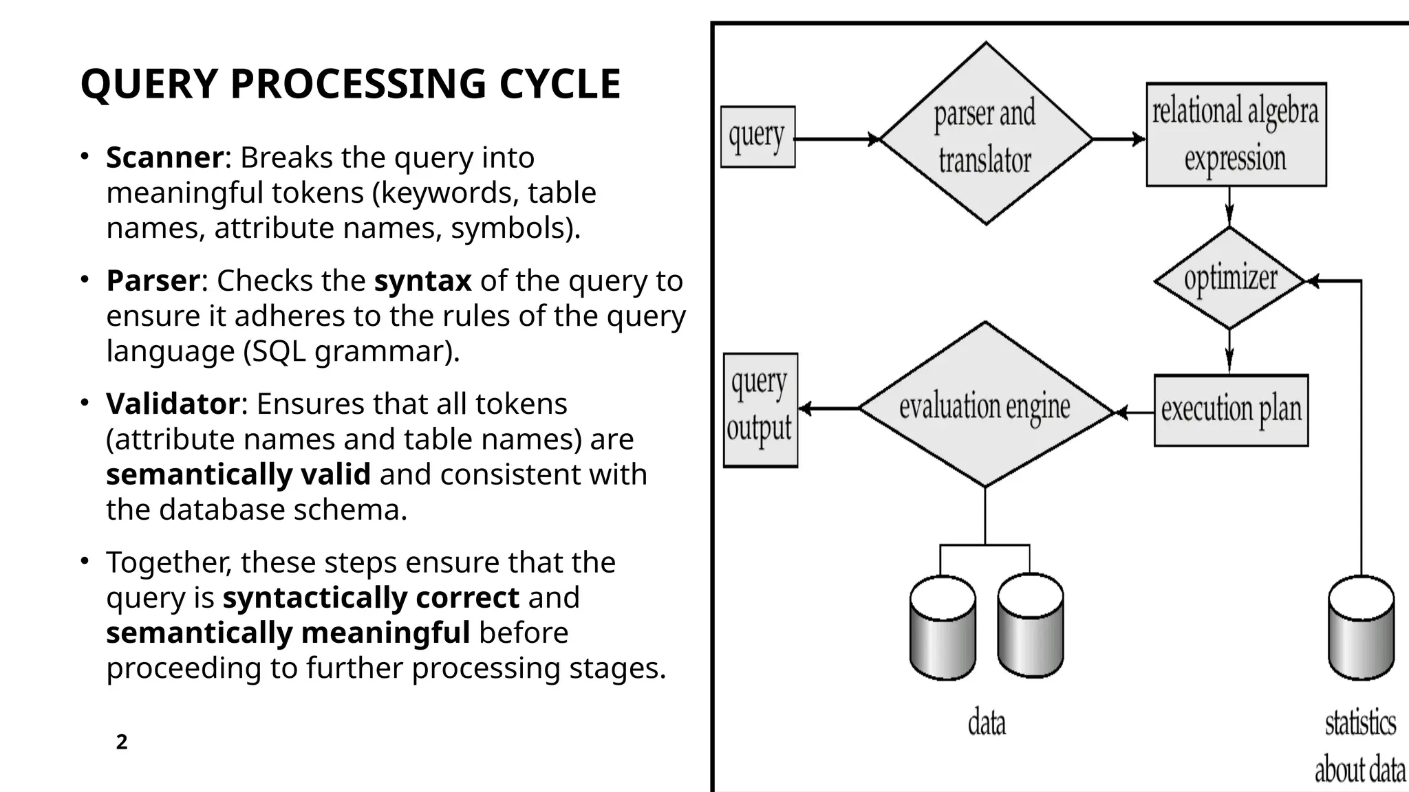
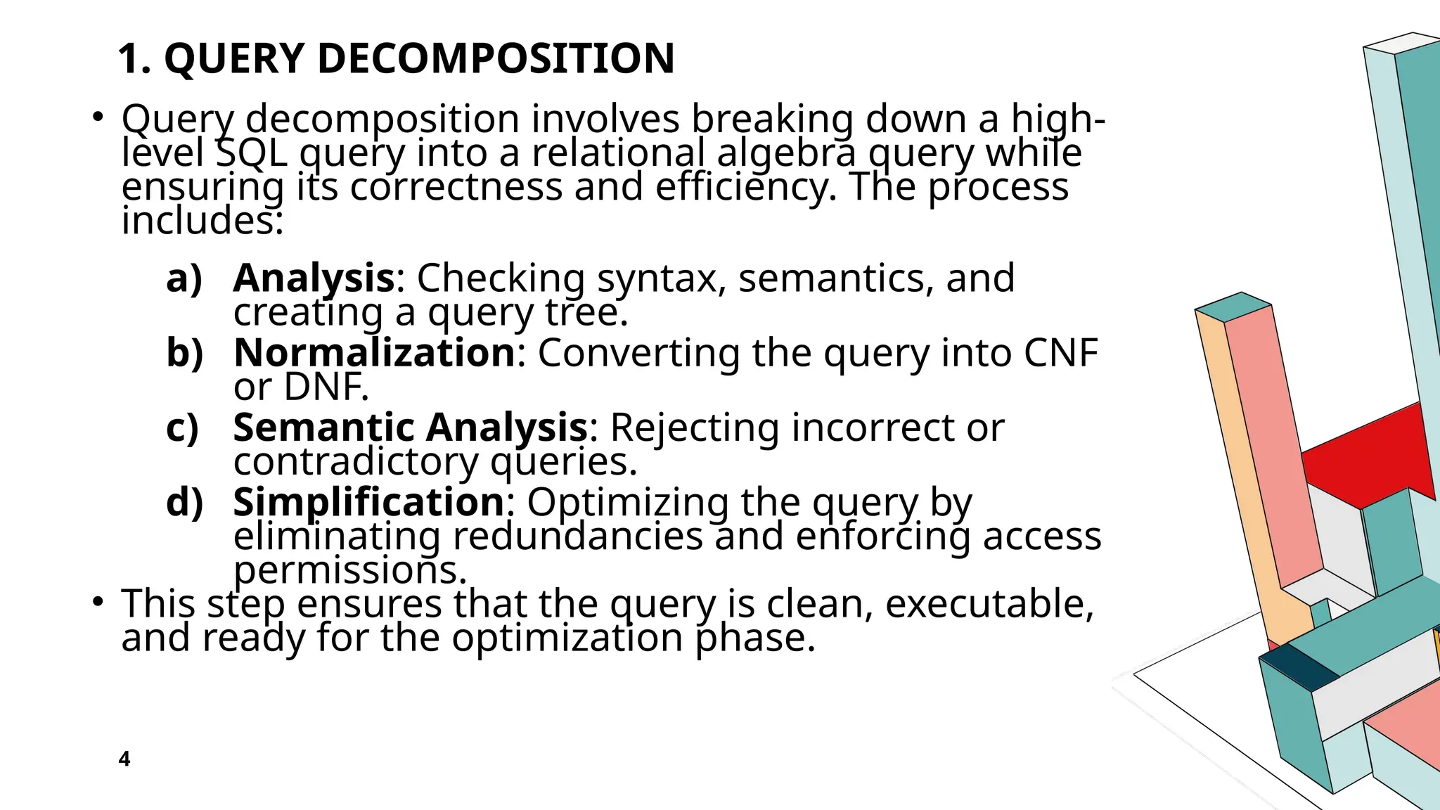
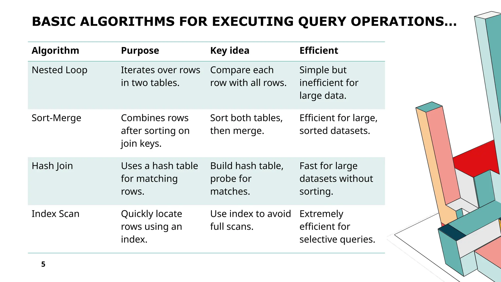
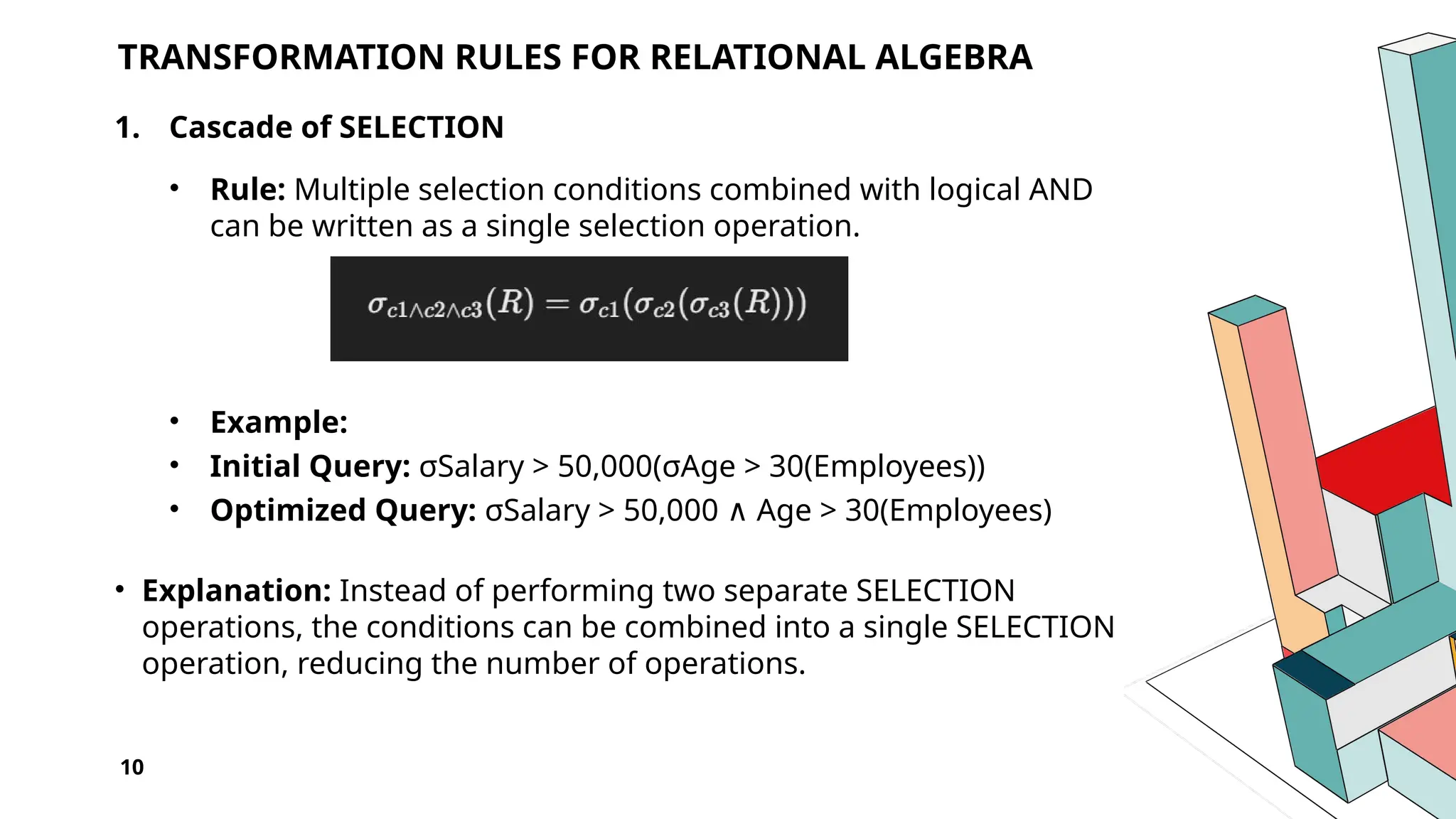
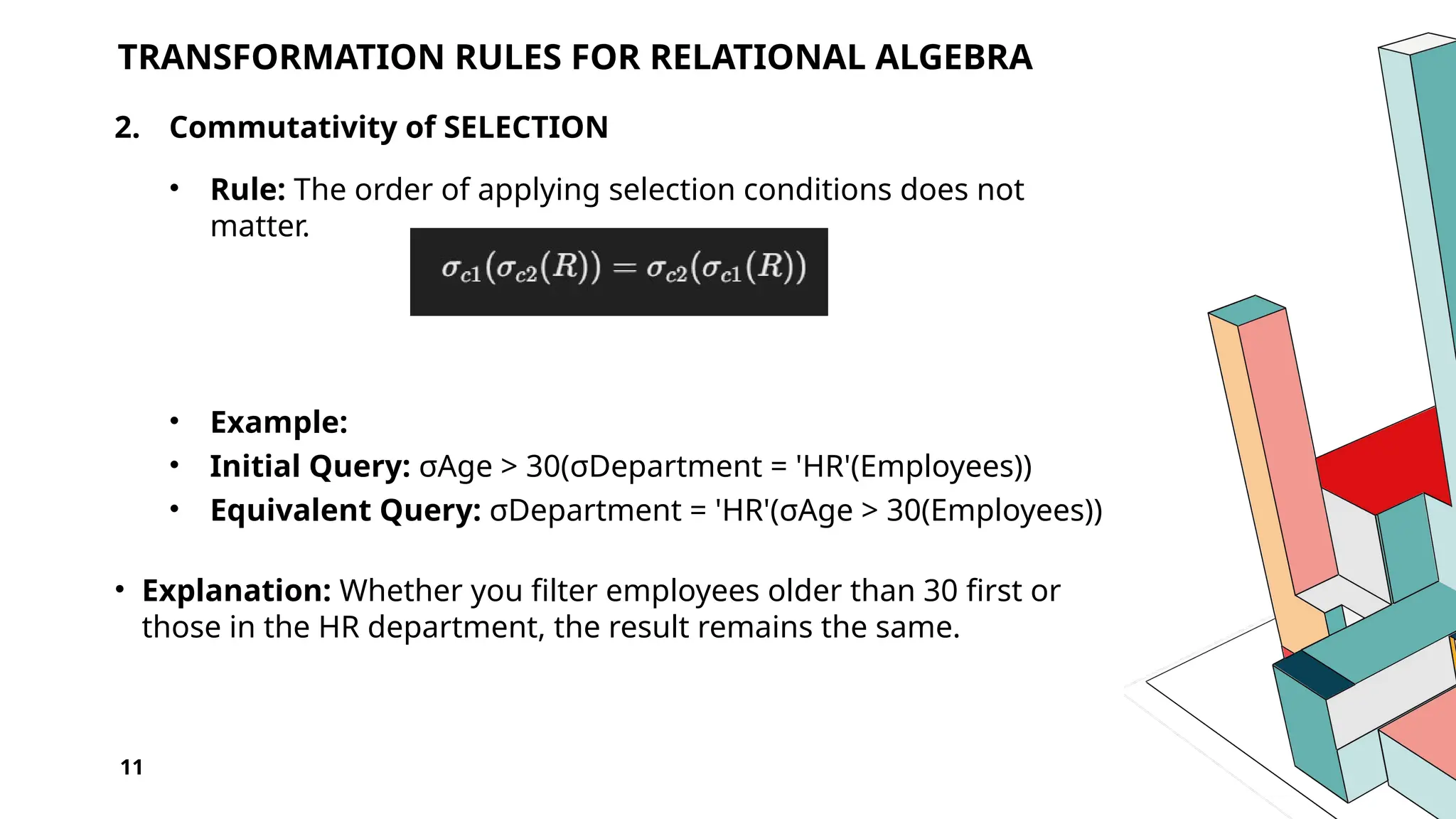
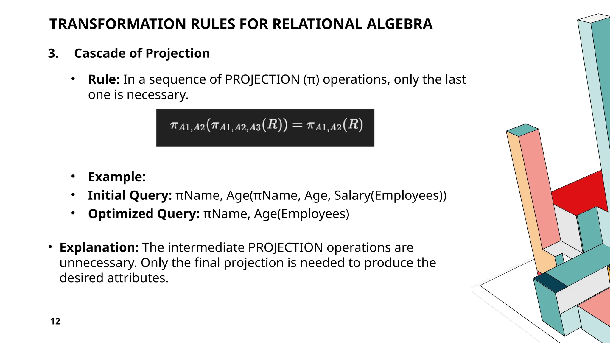
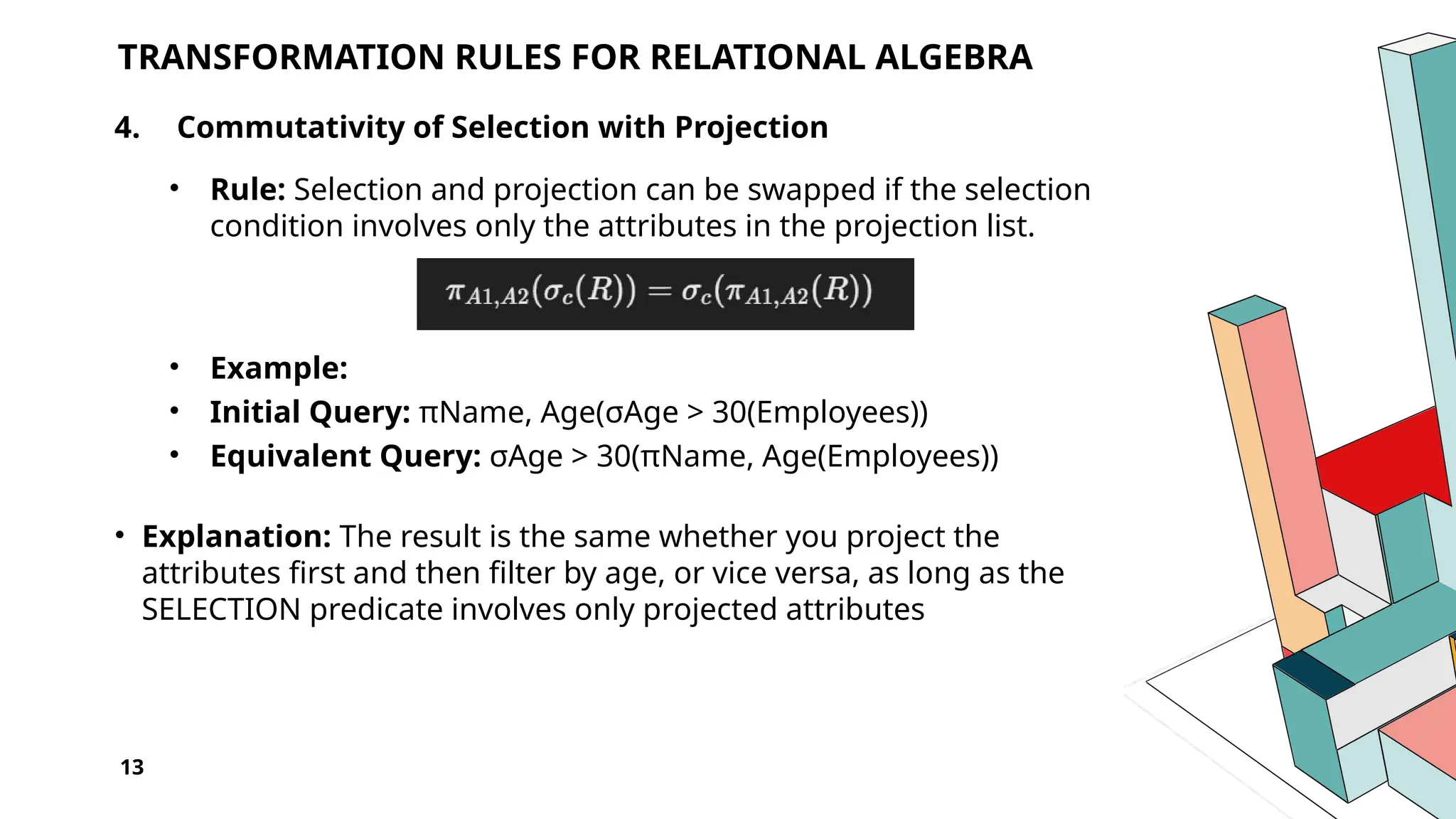
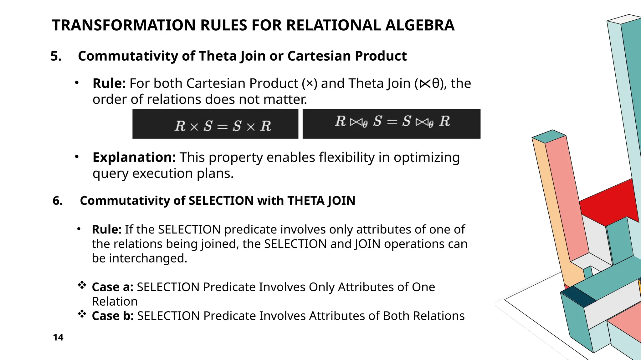
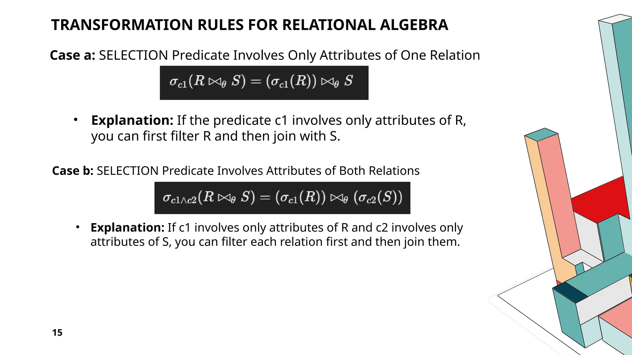
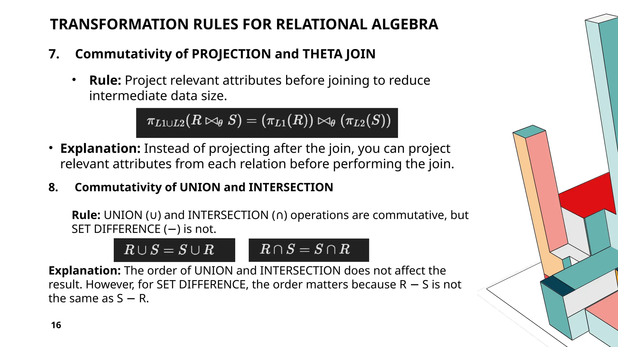
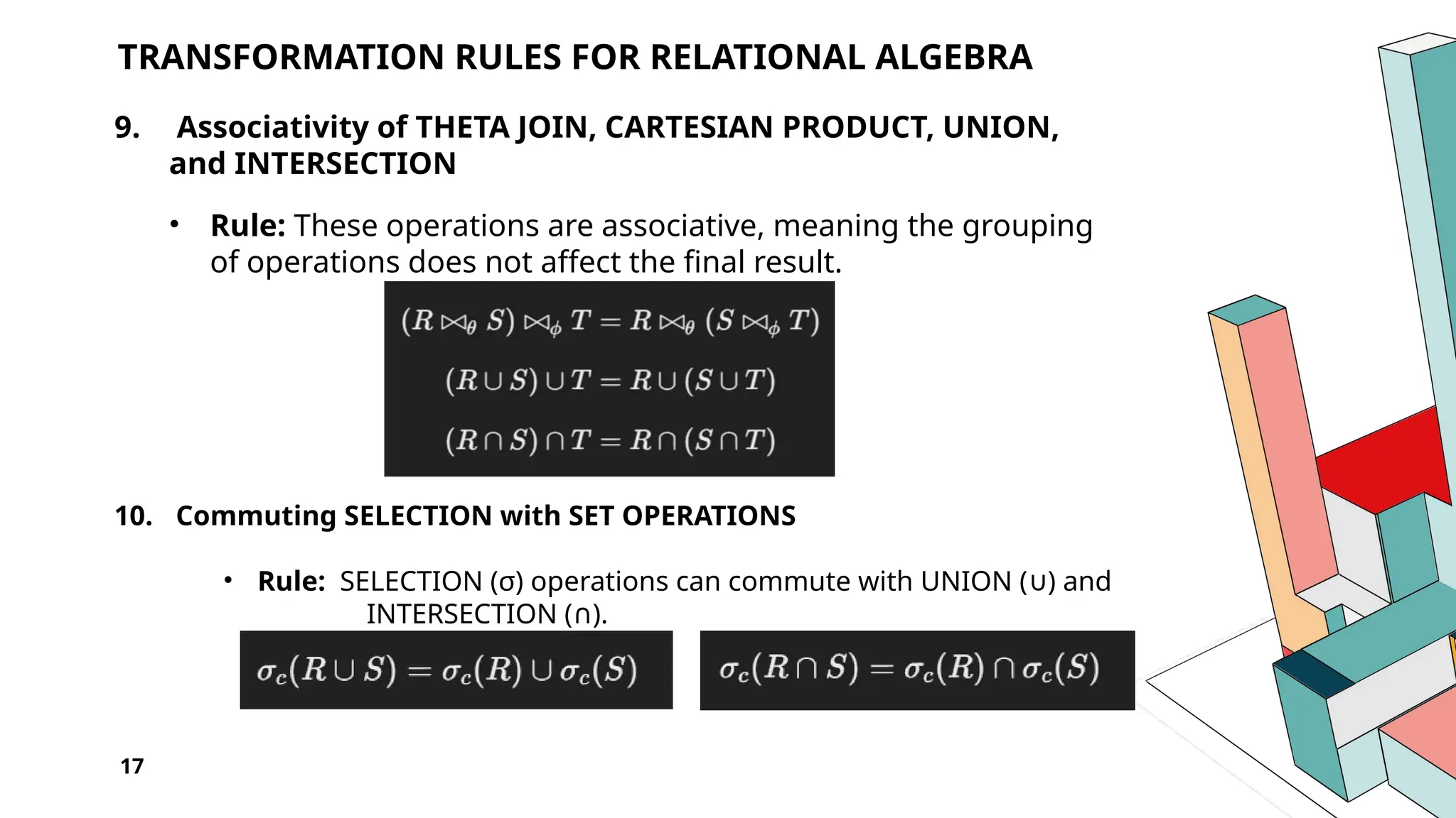
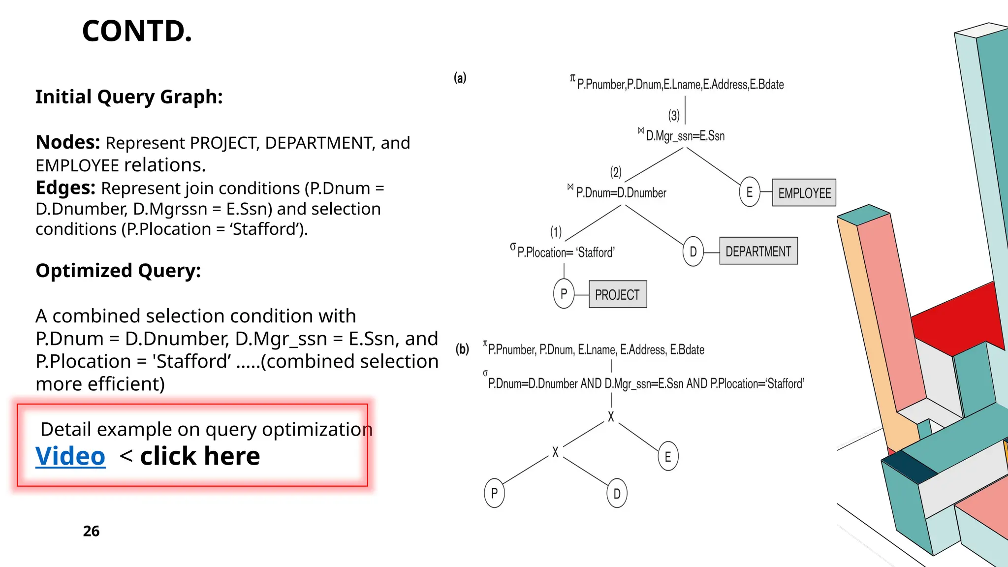
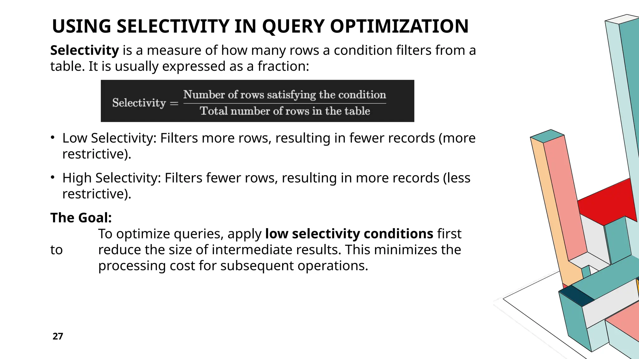


The document outlines the query processing and optimization cycle, detailing the steps of query decomposition, execution strategies, and optimization techniques. It emphasizes the importance of transforming high-level SQL queries into efficient execution plans using various algorithms and optimization rules. Additionally, concepts such as selectivity, cost estimation, and semantic query optimization are discussed to enhance query performance and resource usage.