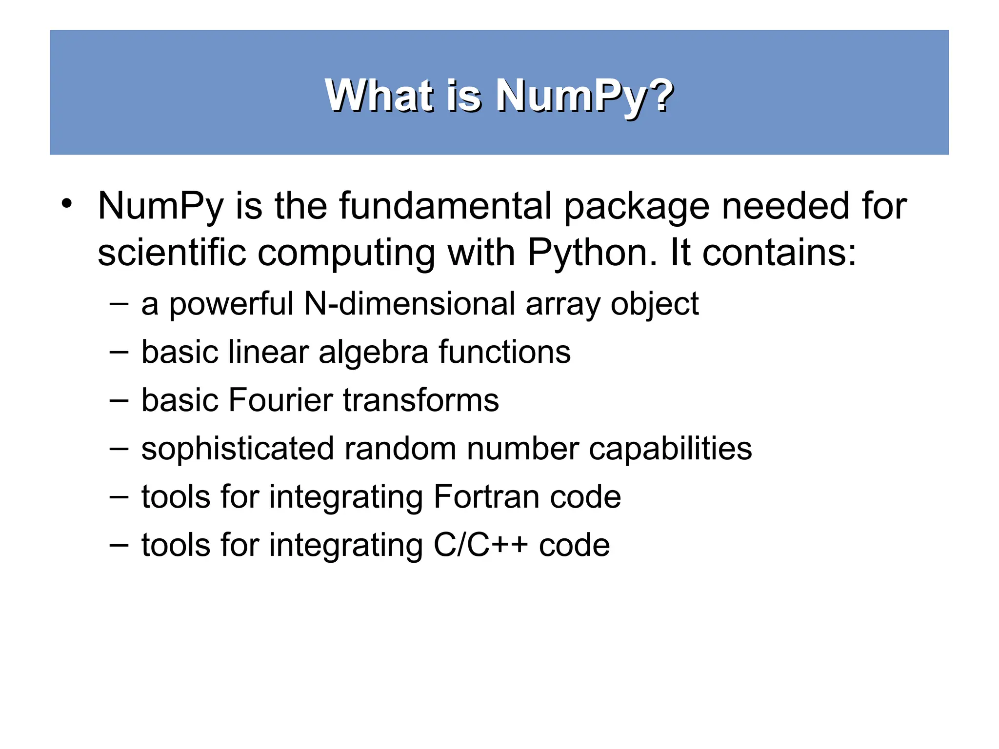
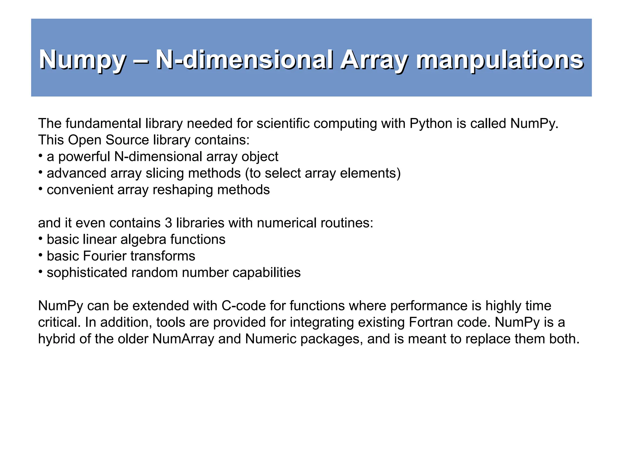
The document provides an overview of NumPy, a fundamental library for scientific computing in Python that includes n-dimensional array objects and various mathematical functions. It covers how to create and manipulate NumPy arrays, highlighting their advantages over Python lists, such as efficiency and support for multidimensional operations. Additionally, it includes examples of creating arrays, utilizing different NumPy functions, and integrating with C and Fortran code.

![Arrays – Numerical Python (Numpy) Arrays – Numerical Python (Numpy) • Lists ok for storing small amounts of one-dimensional data • But, can’t use directly with arithmetical operators (+, -, *, /, …) • Need efficient arrays with arithmetic and better multidimensional tools • Numpy • Similar to lists, but much more capable, except fixed size >>> a = [1,3,5,7,9] >>> print(a[2:4]) [5, 7] >>> b = [[1, 3, 5, 7, 9], [2, 4, 6, 8, 10]] >>> print(b[0]) [1, 3, 5, 7, 9] >>> print(b[1][2:4]) [6, 8] >>> import numpy >>> a = [1,3,5,7,9] >>> b = [3,5,6,7,9] >>> c = a + b >>> print c [1, 3, 5, 7, 9, 3, 5, 6, 7, 9]](https://image.slidesharecdn.com/numpy-1-250111150824-0757d8b7/75/Python-crash-course-libraries-numpy-1-panda-ppt-5-2048.jpg)
![Numpy – Creating vectors Numpy – Creating vectors • From lists – numpy.array # as vectors from lists >>> a = numpy.array([1,3,5,7,9]) >>> b = numpy.array([3,5,6,7,9]) >>> c = a + b >>> print(c) [4, 8, 11, 14, 18] >>> type(c) (<type 'numpy.ndarray'>) >>> c.shape (5,)](https://image.slidesharecdn.com/numpy-1-250111150824-0757d8b7/75/Python-crash-course-libraries-numpy-1-panda-ppt-13-2048.jpg)
![Numpy – Creating matrices Numpy – Creating matrices >>> l = [[1, 2, 3], [3, 6, 9], [2, 4, 6]] # create a list >>> a = numpy.array(l) # convert a list to an array >>>print(a) [[1 2 3] [3 6 9] [2 4 6]] >>> a.shape (3, 3) >>> print(a.dtype) # get type of an array int64 # or directly as matrix >>> M = array([[1, 2], [3, 4]]) >>> M.shape (2,2) >>> M.dtype dtype('int64') #only one type >>> M[0,0] = "hello" Traceback (most recent call last): File "<stdin>", line 1, in <module> ValueError: invalid literal for long() with base 10: 'hello‘ >>> M = numpy.array([[1, 2], [3, 4]], dtype=complex) >>> M array([[ 1.+0.j, 2.+0.j], [ 3.+0.j, 4.+0.j]])](https://image.slidesharecdn.com/numpy-1-250111150824-0757d8b7/75/Python-crash-course-libraries-numpy-1-panda-ppt-14-2048.jpg)
![Numpy – Matrices use Numpy – Matrices use >>> print(a) [[1 2 3] [3 6 9] [2 4 6]] >>> print(a[0]) # this is just like a list of lists [1 2 3] >>> print(a[1, 2]) # arrays can be given comma separated indices 9 >>> print(a[1, 1:3]) # and slices [6 9] >>> print(a[:,1]) [2 6 4] >>> a[1, 2] = 7 >>> print(a) [[1 2 3] [3 6 7] [2 4 6]] >>> a[:, 0] = [0, 9, 8] >>> print(a) [[0 2 3] [9 6 7] [8 4 6]]](https://image.slidesharecdn.com/numpy-1-250111150824-0757d8b7/75/Python-crash-course-libraries-numpy-1-panda-ppt-15-2048.jpg)
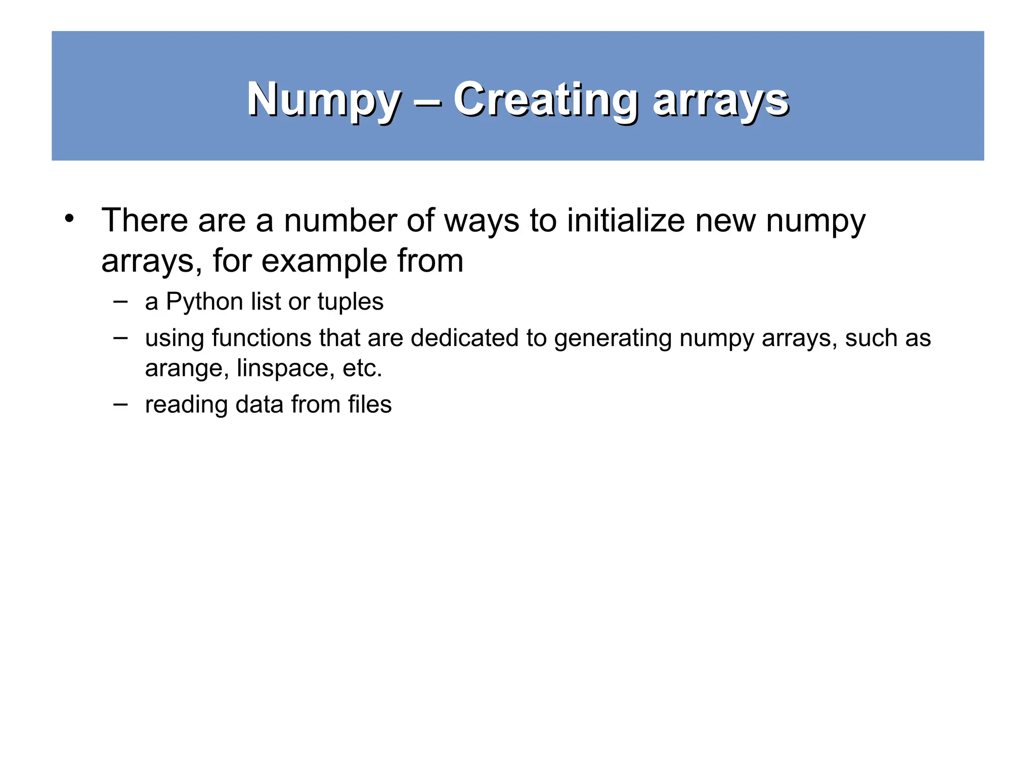
![Numpy – Creating arrays Numpy – Creating arrays • Generation functions >>> x = arange(0, 10, 1) # arguments: start, stop, step >>> x array([0, 1, 2, 3, 4, 5, 6, 7, 8, 9]) >>> numpy.linspace(0, 10, 25) array([ 0. , 0.41666667, 0.83333333, 1.25 , 1.66666667, 2.08333333, 2.5 , 2.91666667, 3.33333333, 3.75 , 4.16666667, 4.58333333, 5. , 5.41666667, 5.83333333, 6.25 , 6.66666667, 7.08333333, 7.5 , 7.91666667, 8.33333333, 8.75 , 9.16666667, 9.58333333, 10. ]) >>> numpy.logspace(0, 10, 10, base=numpy.e) array([ 1.00000000e+00, 3.03773178e+00, 9.22781435e+00, 2.80316249e+01, 8.51525577e+01, 2.58670631e+02, 7.85771994e+02, 2.38696456e+03, 7.25095809e+03, 2.20264658e+04])](https://image.slidesharecdn.com/numpy-1-250111150824-0757d8b7/75/Python-crash-course-libraries-numpy-1-panda-ppt-16-2048.jpg)
![Numpy – Creating arrays Numpy – Creating arrays # a diagonal matrix >>> numpy.diag([1,2,3]) array([[1, 0, 0], [0, 2, 0], [0, 0, 3]]) >>> b = numpy.zeros(5) >>> print(b) [ 0. 0. 0. 0. 0.] >>> b.dtype dtype(‘float64’) >>> n = 1000 >>> my_int_array = numpy.zeros(n, dtype=numpy.int) >>> my_int_array.dtype dtype(‘int32’) >>> c = numpy.ones((3,3)) >>> c array([[ 1., 1., 1.], [ 1., 1., 1.], [ 1., 1., 1.]])](https://image.slidesharecdn.com/numpy-1-250111150824-0757d8b7/75/Python-crash-course-libraries-numpy-1-panda-ppt-17-2048.jpg)
![Numpy – array creation and use Numpy – array creation and use >>> d = numpy.arange(5) # just like range() >>> print(d) [0 1 2 3 4] >>> d[1] = 9.7 >>> print(d) # arrays keep their type even if elements changed [0 9 2 3 4] >>> print(d*0.4) # operations create a new array, with new type [ 0. 3.6 0.8 1.2 1.6] >>> d = numpy.arange(5, dtype=numpy.float) >>> print(d) [ 0. 1. 2. 3. 4.] >>> numpy.arange(3, 7, 0.5) # arbitrary start, stop and step array([ 3. , 3.5, 4. , 4.5, 5. , 5.5, 6. , 6.5])](https://image.slidesharecdn.com/numpy-1-250111150824-0757d8b7/75/Python-crash-course-libraries-numpy-1-panda-ppt-18-2048.jpg)
![Numpy – array creation and use Numpy – array creation and use >>> x, y = numpy.mgrid[0:5, 0:5] # similar to meshgrid in MATLAB >>> x array([[0, 0, 0, 0, 0], [1, 1, 1, 1, 1], [2, 2, 2, 2, 2], [3, 3, 3, 3, 3], [4, 4, 4, 4, 4]]) # random data >>> numpy.random.rand(5,5) array([[ 0.51531133, 0.74085206, 0.99570623, 0.97064334, 0.5819413 ], [ 0.2105685 , 0.86289893, 0.13404438, 0.77967281, 0.78480563], [ 0.62687607, 0.51112285, 0.18374991, 0.2582663 , 0.58475672], [ 0.72768256, 0.08885194, 0.69519174, 0.16049876, 0.34557215], [ 0.93724333, 0.17407127, 0.1237831 , 0.96840203, 0.52790012]])](https://image.slidesharecdn.com/numpy-1-250111150824-0757d8b7/75/Python-crash-course-libraries-numpy-1-panda-ppt-19-2048.jpg)
![Numpy – Creating arrays Numpy – Creating arrays >>> M = numpy.random.rand(3,3) >>> M array([[ 0.84188778, 0.70928643, 0.87321035], [ 0.81885553, 0.92208501, 0.873464 ], [ 0.27111984, 0.82213106, 0.55987325]]) >>> >>> numpy.save('saved-matrix.npy', M) >>> numpy.load('saved-matrix.npy') array([[ 0.84188778, 0.70928643, 0.87321035], [ 0.81885553, 0.92208501, 0.873464 ], [ 0.27111984, 0.82213106, 0.55987325]]) >>> >>> os.system('head saved-matrix.npy') NUMPYF{'descr': '<f8', 'fortran_order': False, 'shape': (3, 3), } Ï< £¾ðê? sy²æ?$÷ÒVñë?Ù4ê?%dn¸í?Ã[Äjóë?Ä,ZÑ?Ç ÎåNê?ó7L{êá?0 >>>](https://image.slidesharecdn.com/numpy-1-250111150824-0757d8b7/75/Python-crash-course-libraries-numpy-1-panda-ppt-21-2048.jpg)
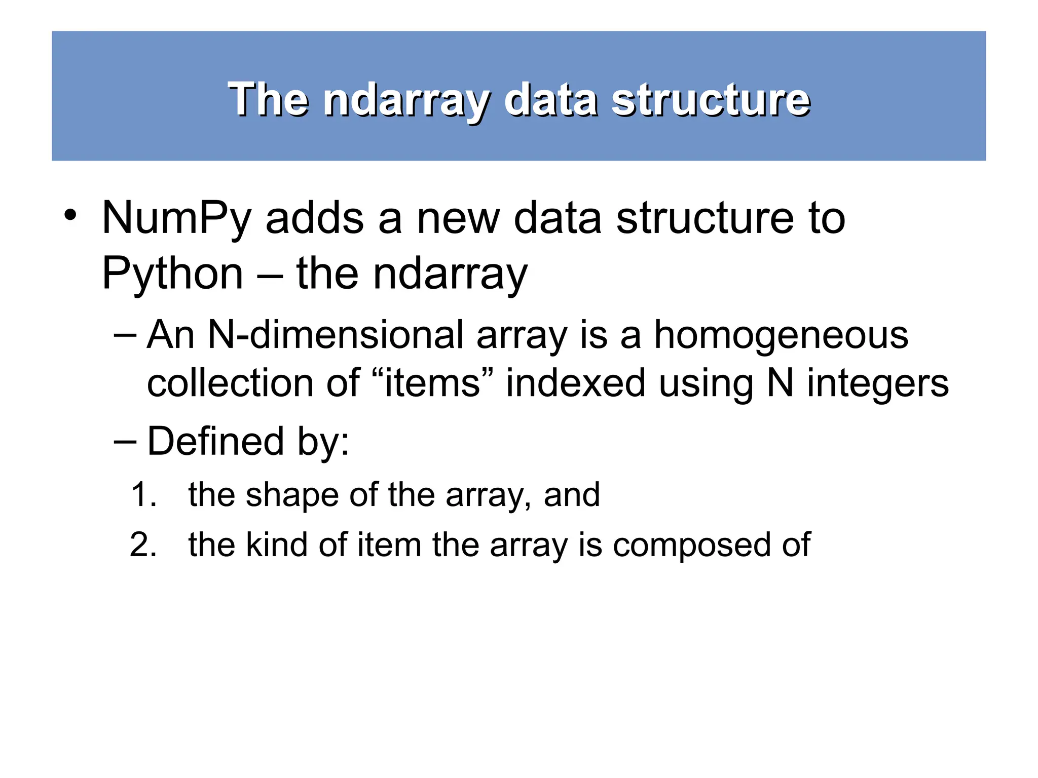
![Numpy - ndarray Numpy - ndarray • NumPy's main object is the homogeneous multidimensional array called ndarray. – This is a table of elements (usually numbers), all of the same type, indexed by a tuple of positive integers. Typical examples of multidimensional arrays include vectors, matrices, images and spreadsheets. – Dimensions usually called axes, number of axes is the rank [7, 5, -1] An array of rank 1 i.e. It has 1 axis of length 3 [ [ 1.5, 0.2, -3.7] , An array of rank 2 i.e. It has 2 axes, the first [ 0.1, 1.7, 2.9] ] length 3, the second of length 3 (a matrix with 2 rows and 3 columns](https://image.slidesharecdn.com/numpy-1-250111150824-0757d8b7/75/Python-crash-course-libraries-numpy-1-panda-ppt-22-2048.jpg)
![Numpy – array creation and use Numpy – array creation and use >>> x = np.array([1,2,3,4]) >>> y = x >>> x is y True >>> id(x), id(y) (139814289111920, 139814289111920) >>> x[0] = 9 >>> y array([9, 2, 3, 4]) >>> x[0] = 1 >>> z = x[:] >>> x is z False >>> id(x), id(z) (139814289111920, 139814289112080) >>> x[0] = 8 >>> z array([8, 2, 3, 4]) Two ndarrays are mutable and may be views to the same memory: >>> x = np.array([1,2,3,4]) >>> y = x.copy() >>> x is y False >>> id(x), id(y) (139814289111920, 139814289111840) >>> x[0] = 9 >>> x array([9, 2, 3, 4]) >>> y array([1, 2, 3, 4])](https://image.slidesharecdn.com/numpy-1-250111150824-0757d8b7/75/Python-crash-course-libraries-numpy-1-panda-ppt-24-2048.jpg)
![Numpy – array creation and use Numpy – array creation and use >>> a = numpy.arange(4.0) >>> b = a * 23.4 >>> c = b/(a+1) >>> c += 10 >>> print c [ 10. 21.7 25.6 27.55] >>> arr = numpy.arange(100, 200) >>> select = [5, 25, 50, 75, -5] >>> print(arr[select]) # can use integer lists as indices [105, 125, 150, 175, 195] >>> arr = numpy.arange(10, 20 ) >>> div_by_3 = arr%3 == 0 # comparison produces boolean array >>> print(div_by_3) [ False False True False False True False False True False] >>> print(arr[div_by_3]) # can use boolean lists as indices [12 15 18] >>> arr = numpy.arange(10, 20) . reshape((2,5)) [[10 11 12 13 14] [15 16 17 18 19]]](https://image.slidesharecdn.com/numpy-1-250111150824-0757d8b7/75/Python-crash-course-libraries-numpy-1-panda-ppt-25-2048.jpg)
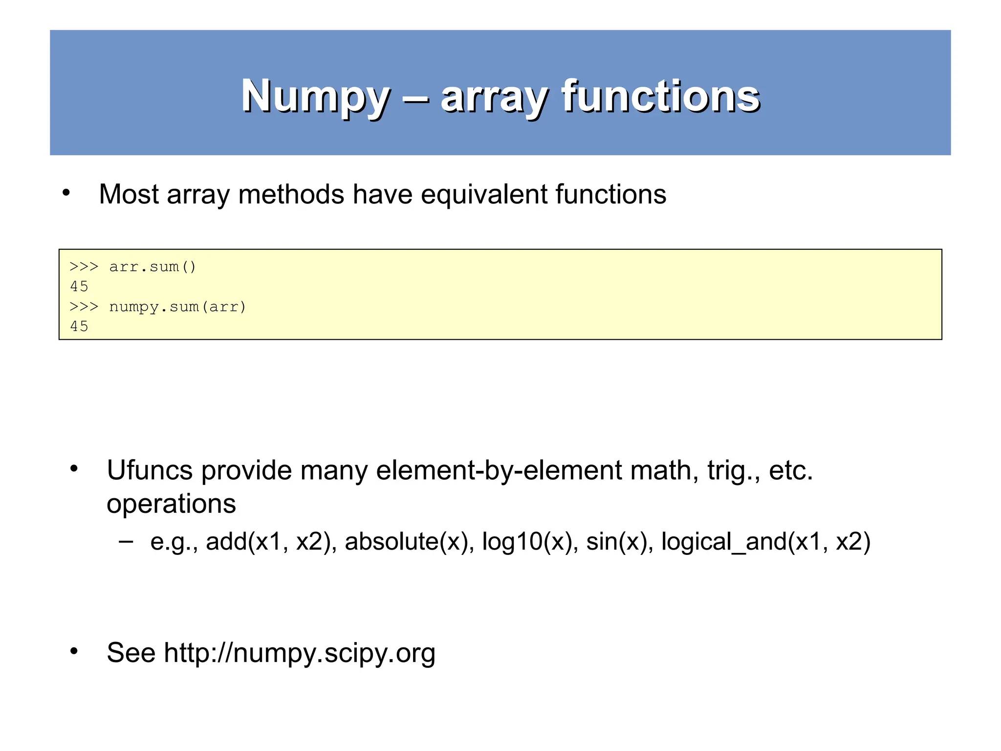
![Numpy – array methods Numpy – array methods >>> arr.sum() 145 >>> arr.mean() 14.5 >>> arr.std() 2.8722813232690143 >>> arr.max() 19 >>> arr.min() 10 >>> div_by_3.all() False >>> div_by_3.any() True >>> div_by_3.sum() 3 >>> div_by_3.nonzero() (array([2, 5, 8]),)](https://image.slidesharecdn.com/numpy-1-250111150824-0757d8b7/75/Python-crash-course-libraries-numpy-1-panda-ppt-26-2048.jpg)
![Numpy – array methods - sorting Numpy – array methods - sorting >>> arr = numpy.array([4.5, 2.3, 6.7, 1.2, 1.8, 5.5]) >>> arr.sort() # acts on array itself >>> print(arr) [ 1.2 1.8 2.3 4.5 5.5 6.7] >>> x = numpy.array([4.5, 2.3, 6.7, 1.2, 1.8, 5.5]) >>> numpy.sort(x) array([ 1.2, 1.8, 2.3, 4.5, 5.5, 6.7]) >>> print(x) [ 4.5 2.3 6.7 1.2 1.8 5.5] >>> s = x.argsort() >>> s array([3, 4, 1, 0, 5, 2]) >>> x[s] array([ 1.2, 1.8, 2.3, 4.5, 5.5, 6.7]) >>> y[s] array([ 6.2, 7.8, 2.3, 1.5, 8.5, 4.7])](https://image.slidesharecdn.com/numpy-1-250111150824-0757d8b7/75/Python-crash-course-libraries-numpy-1-panda-ppt-27-2048.jpg)
![Numpy – array operations Numpy – array operations >>> a = array([[1.0, 2.0], [4.0, 3.0]]) >>> print a [[ 1. 2.] [ 3. 4.]] >>> a.transpose() array([[ 1., 3.], [ 2., 4.]]) >>> inv(a) array([[-2. , 1. ], [ 1.5, -0.5]]) >>> u = eye(2) # unit 2x2 matrix; "eye" represents "I" >>> u array([[ 1., 0.], [ 0., 1.]]) >>> j = array([[0.0, -1.0], [1.0, 0.0]]) >>> dot (j, j) # matrix product array([[-1., 0.], [ 0., -1.]])](https://image.slidesharecdn.com/numpy-1-250111150824-0757d8b7/75/Python-crash-course-libraries-numpy-1-panda-ppt-29-2048.jpg)
![Numpy – statistics Numpy – statistics >>> a = np.array([1, 4, 3, 8, 9, 2, 3], float) >>> np.median(a) 3.0 >>> a = np.array([[1, 2, 1, 3], [5, 3, 1, 8]], float) >>> c = np.corrcoef(a) >>> c array([[ 1. , 0.72870505], [ 0.72870505, 1. ]]) >>> np.cov(a) array([[ 0.91666667, 2.08333333], [ 2.08333333, 8.91666667]]) In addition to the mean, var, and std functions, NumPy supplies several other methods for returning statistical features of arrays. The median can be found: The correlation coefficient for multiple variables observed at multiple instances can be found for arrays of the form [[x1, x2, …], [y1, y2, …], [z1, z2, …], …] where x, y, z are different observables and the numbers indicate the observation times: Here the return array c[i,j] gives the correlation coefficient for the ith and jth observables. Similarly, the covariance for data can be found::](https://image.slidesharecdn.com/numpy-1-250111150824-0757d8b7/75/Python-crash-course-libraries-numpy-1-panda-ppt-30-2048.jpg)
![Numpy – arrays, matrices Numpy – arrays, matrices >>> import numpy >>> m = numpy.mat([[1,2],[3,4]]) or >>> a = numpy.array([[1,2],[3,4]]) >>> m = numpy.mat(a) or >>> a = numpy.array([[1,2],[3,4]]) >>> m = numpy.asmatrix(a) For two dimensional arrays NumPy defined a special matrix class in module matrix. Objects are created either with matrix() or mat() or converted from an array with method asmatrix(). Note that the statement m = mat(a) creates a copy of array 'a'. Changing values in 'a' will not affect 'm'. On the other hand, method m = asmatrix(a) returns a new reference to the same data. Changing values in 'a' will affect matrix 'm'.](https://image.slidesharecdn.com/numpy-1-250111150824-0757d8b7/75/Python-crash-course-libraries-numpy-1-panda-ppt-32-2048.jpg)
![Numpy – matrices Numpy – matrices >>> a = array([[1,2],[3,4]]) >>> m = mat(a) # convert 2-d array to matrix >>> m = matrix([[1, 2], [3, 4]]) >>> a[0] # result is 1-dimensional array([1, 2]) >>> m[0] # result is 2-dimensional matrix([[1, 2]]) >>> a*a # element-by-element multiplication array([[ 1, 4], [ 9, 16]]) >>> m*m # (algebraic) matrix multiplication matrix([[ 7, 10], [15, 22]]) >>> a**3 # element-wise power array([[ 1, 8], [27, 64]]) >>> m**3 # matrix multiplication m*m*m matrix([[ 37, 54], [ 81, 118]]) >>> m.T # transpose of the matrix matrix([[1, 3], [2, 4]]) >>> m.H # conjugate transpose (differs from .T for complex matrices) matrix([[1, 3], [2, 4]]) >>> m.I # inverse matrix matrix([[-2. , 1. ], [ 1.5, -0.5]]) Array and matrix operations may be quite different!](https://image.slidesharecdn.com/numpy-1-250111150824-0757d8b7/75/Python-crash-course-libraries-numpy-1-panda-ppt-33-2048.jpg)
![Numpy – matrices Numpy – matrices • Operator *, dot(), and multiply(): • For array, '*' means element-wise multiplication, and the dot() function is used for matrix multiplication. • For matrix, '*'means matrix multiplication, and the multiply() function is used for element-wise multiplication. • Handling of vectors (rank-1 arrays) • For array, the vector shapes 1xN, Nx1, and N are all different things. Operations like A[:,1] return a rank-1 array of shape N, not a rank-2 of shape Nx1. Transpose on a rank-1 array does nothing. • For matrix, rank-1 arrays are always upgraded to 1xN or Nx1 matrices (row or column vectors). A[:,1] returns a rank-2 matrix of shape Nx1. • Handling of higher-rank arrays (rank > 2) • array objects can have rank > 2. • matrix objects always have exactly rank 2. • Convenience attributes • array has a .T attribute, which returns the transpose of the data. • matrix also has .H, .I, and .A attributes, which return the conjugate transpose, inverse, and asarray() of the matrix, respectively. • Convenience constructor • The array constructor takes (nested) Python sequences as initializers. As in array([[1,2,3],[4,5,6]]). • The matrix constructor additionally takes a convenient string initializer. As in matrix("[1 2 3; 4 5 6]")](https://image.slidesharecdn.com/numpy-1-250111150824-0757d8b7/75/Python-crash-course-libraries-numpy-1-panda-ppt-34-2048.jpg)
![Numpy – array mathematics Numpy – array mathematics >>> a = np.array([1,2,3], float) >>> b = np.array([5,2,6], float) >>> a + b array([6., 4., 9.]) >>> a – b array([-4., 0., -3.]) >>> a * b array([5., 4., 18.]) >>> b / a array([5., 1., 2.]) >>> a % b array([1., 0., 3.]) >>> b**a array([5., 4., 216.]) >>> a = np.array([[1, 2], [3, 4], [5, 6]], float) >>> b = np.array([-1, 3], float) >>> a array([[ 1., 2.], [ 3., 4.], [ 5., 6.]]) >>> b array([-1., 3.]) >>> a + b array([[ 0., 5.], [ 2., 7.], [ 4., 9.]]) >>> a = np.array([[1, 2], [3, 4], [5, 6]], float) >>> b = np.array([-1, 3], float) >>> a * a array([[ 1., 4.], [ 9., 16.], [ 25., 36.]]) >>> b * b array([ 1., 9.]) >>> a * b array([[ -1., 6.], [ -3., 12.], [ -5., 18.]]) >>>](https://image.slidesharecdn.com/numpy-1-250111150824-0757d8b7/75/Python-crash-course-libraries-numpy-1-panda-ppt-35-2048.jpg)
![Numpy – array mathematics Numpy – array mathematics >>> A = np.array([[n+m*10 for n in range(5)] for m in range(5)]) >>> v1 = arange(0, 5) >>> A array([[ 0, 1, 2, 3, 4], [10, 11, 12, 13, 14], [20, 21, 22, 23, 24], [30, 31, 32, 33, 34], [40, 41, 42, 43, 44]]) >>> v1 array([0, 1, 2, 3, 4]) >>> np.dot(A,A) array([[ 300, 310, 320, 330, 340], [1300, 1360, 1420, 1480, 1540], [2300, 2410, 2520, 2630, 2740], [3300, 3460, 3620, 3780, 3940], [4300, 4510, 4720, 4930, 5140]]) >>> >>> np.dot(A,v1) array([ 30, 130, 230, 330, 430]) >>> np.dot(v1,v1) 30 >>> Alternatively, we can cast the array objects to the type matrix. This changes the behavior of the standard arithmetic operators +, -, * to use matrix algebra. >>> M = np.matrix(A) >>> v = np.matrix(v1).T >>> v matrix([[0], [1], [2], [3], [4]]) >>> M*v matrix([[ 30], [130], [230], [330], [430]]) >>> v.T * v # inner product matrix([[30]]) # standard matrix algebra applies >>> v + M*v matrix([[ 30], [131], [232], [333], [434]])](https://image.slidesharecdn.com/numpy-1-250111150824-0757d8b7/75/Python-crash-course-libraries-numpy-1-panda-ppt-36-2048.jpg)