

![Characteristic Function in the Case of Crisp Sets and Fuzzy Sets P: X {0,1} P(x) = A : X [0,1] A = {X, A(x)} if x X A Fuzzy Set is a generalized set to which objects can belongs with various degrees (grades) of memberships over the interval [0,1]. Xx Xx if0 if1](https://image.slidesharecdn.com/optimizationusingsoftcomputing-171208092056/75/Optimization-using-soft-computing-17-2048.jpg)
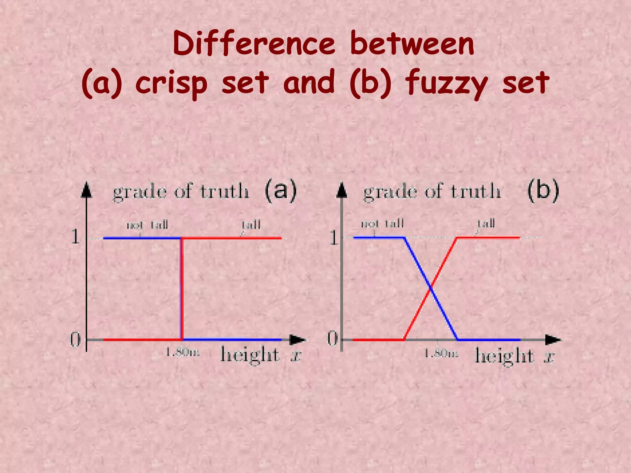
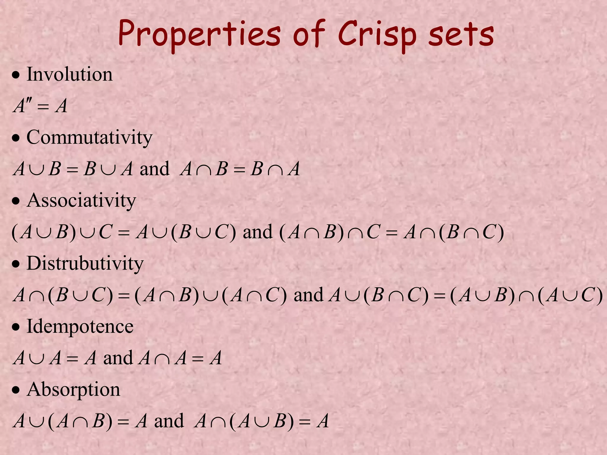
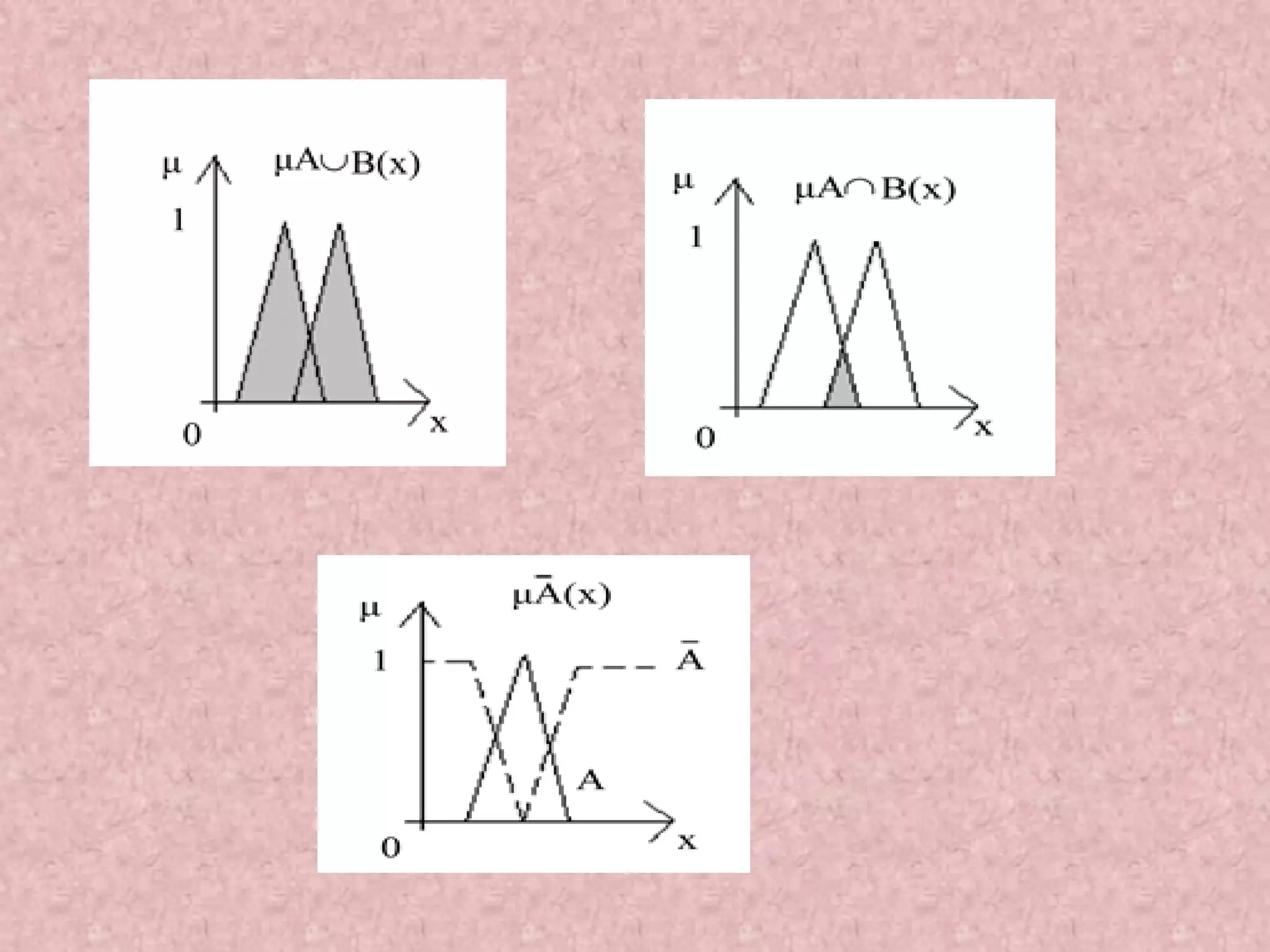
![• Crisp set: This is defined in such a way as to dichotomize the individuals in some given universe of discourse into the two groups- members and nonmembers. Full membership and full non-membership in the fuzzy set can still be indicated by the values 1 and 0, respectively. • Fuzzy set: Mathematically, if U is the universe discourse, the fuzzy set is defined as a pair given as For each , the value is called a grade of membership of x in . Here is called membership function of fuzzy set A. We can consider the concept of a crisp set to be a restricted case of the more general concept of a fuzzy set. ,A ]1,0[: AA Ux )(x ,A ](https://image.slidesharecdn.com/optimizationusingsoftcomputing-171208092056/75/Optimization-using-soft-computing-19-2048.jpg)
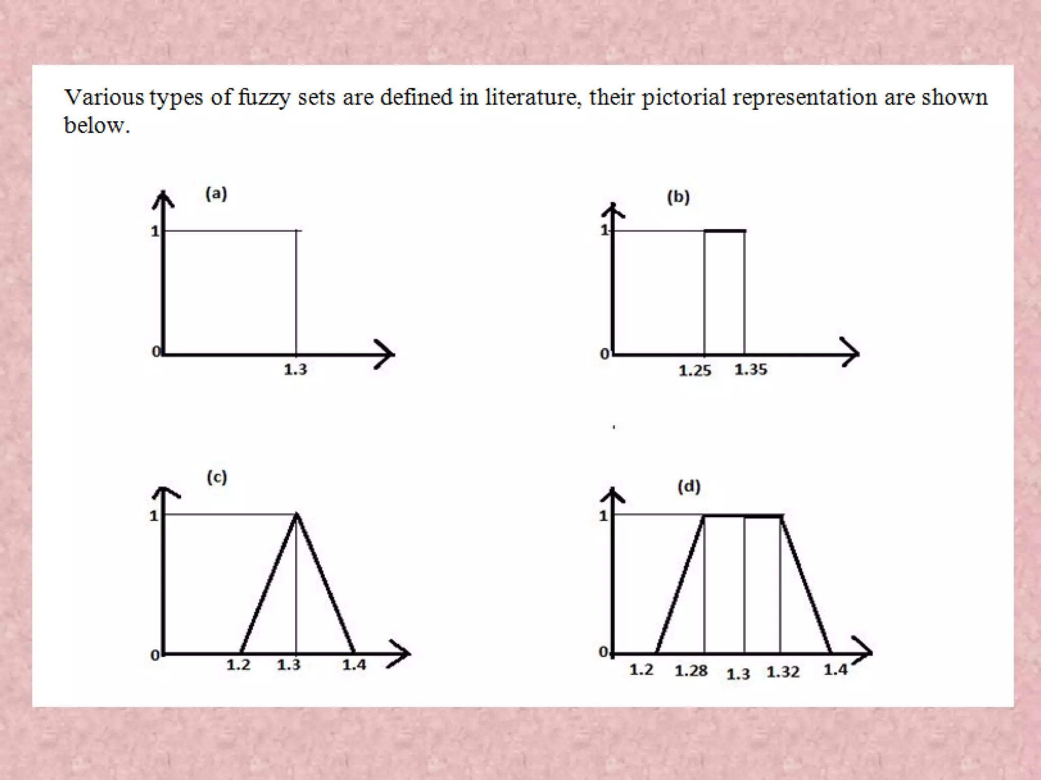
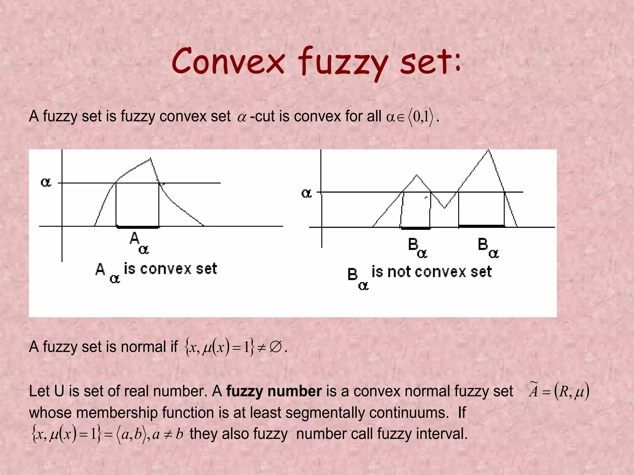
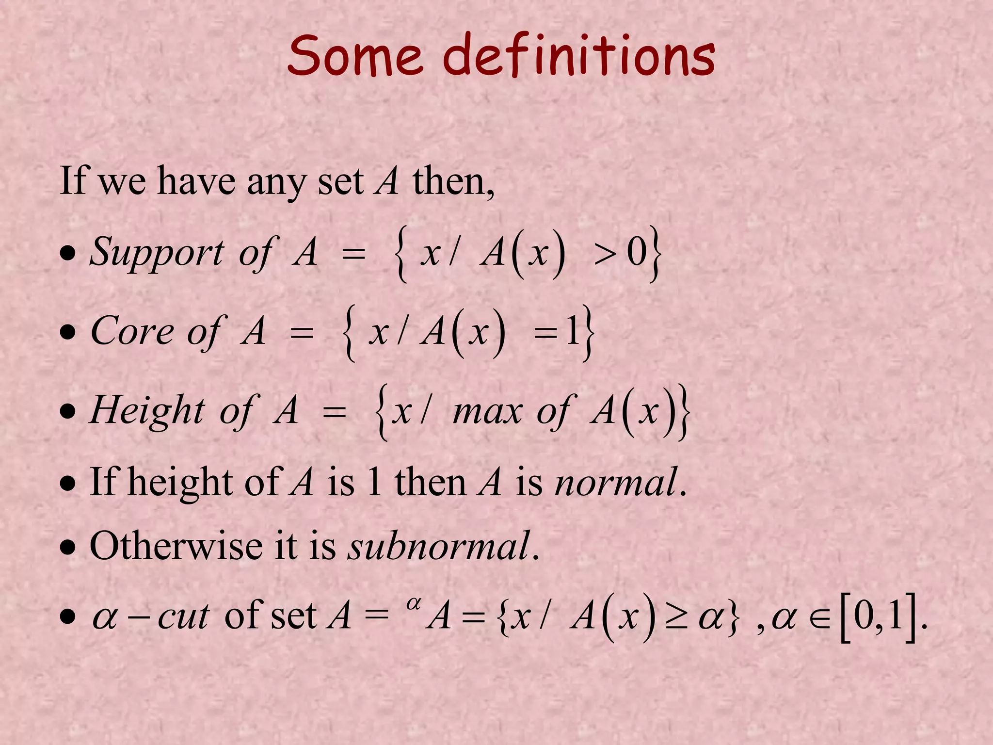
![Some Concepts 1 0 a b X = [a,b] core(A) supp(A) height(A) = 1 (normal fuzzy set) Membership function has a trapezoidal form](https://image.slidesharecdn.com/optimizationusingsoftcomputing-171208092056/75/Optimization-using-soft-computing-28-2048.jpg)
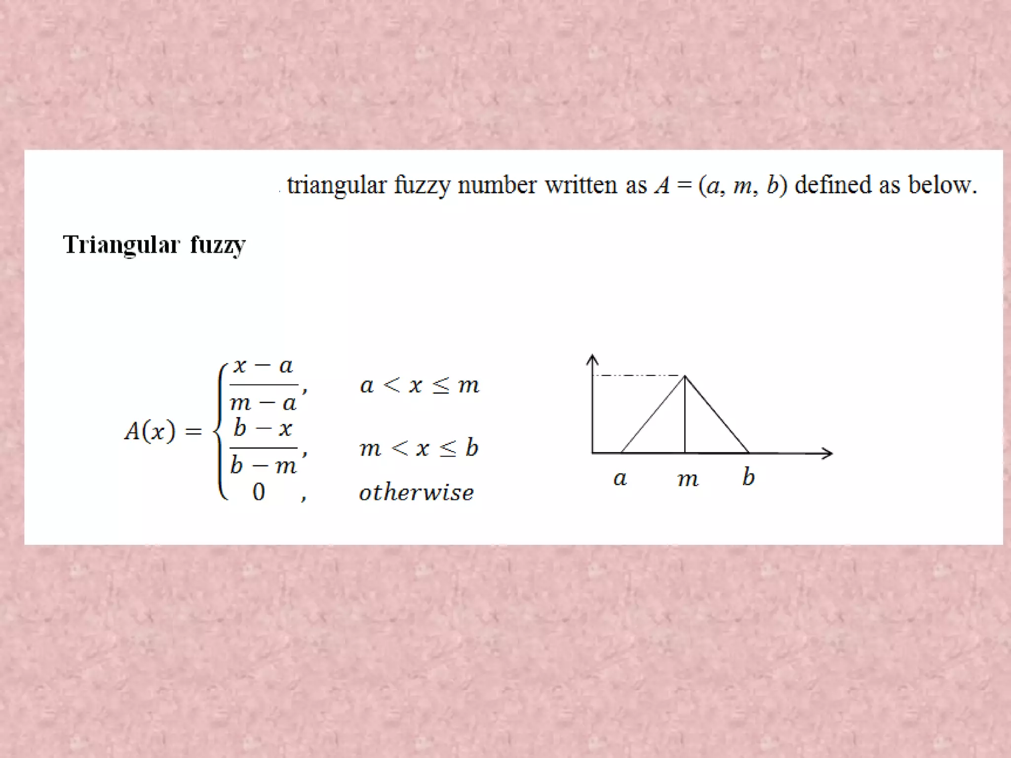
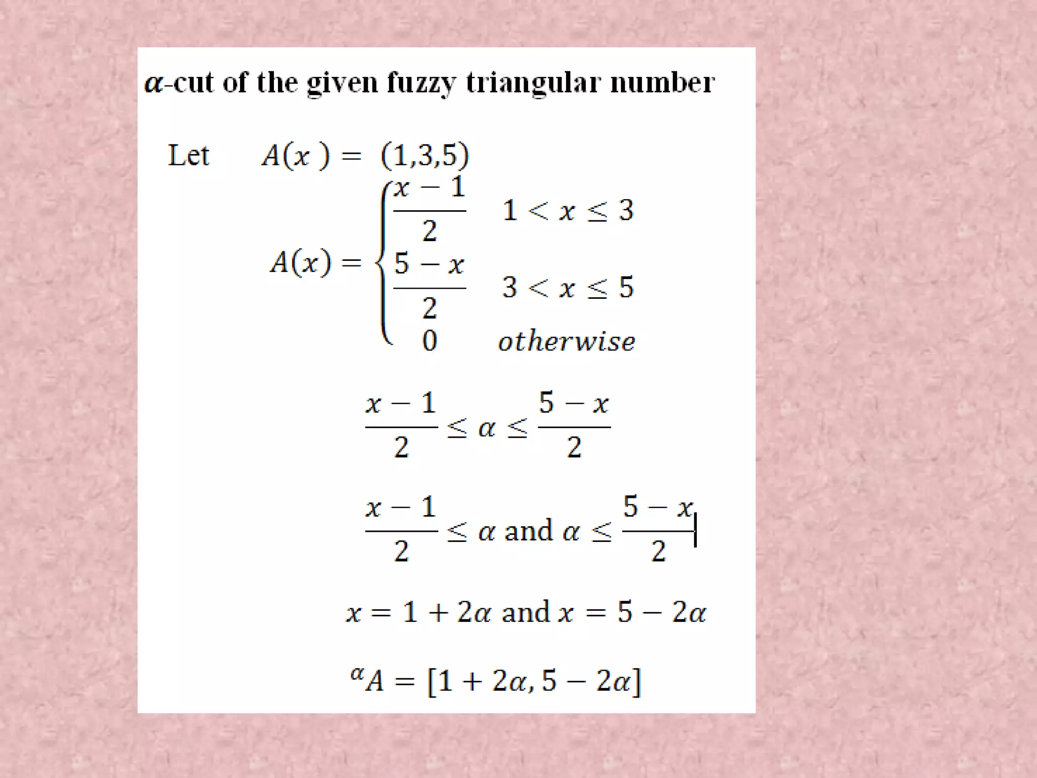
![Fuzzy number in parametric form Parametric representation has advantage of allowing flexible and easy to control shapes of the fuzzy number. A fuzzy number in parametric form is an order pair of the form u = (𝑢 α , 𝑢(α))where 0 ≤ α ≤ 1 satisfying the following conditions: 𝑢 α is a bounded left continuous increasing function in the interval [0, 1] 𝑢 α is a bounded right continuous decreasing function in the interval [0, 1] 𝑢 α ≤ 𝑢(α), α ∈ 0,1 . If for each α, 𝑢 α = 𝑢 α then 𝑢 is a crisp number.](https://image.slidesharecdn.com/optimizationusingsoftcomputing-171208092056/75/Optimization-using-soft-computing-33-2048.jpg)
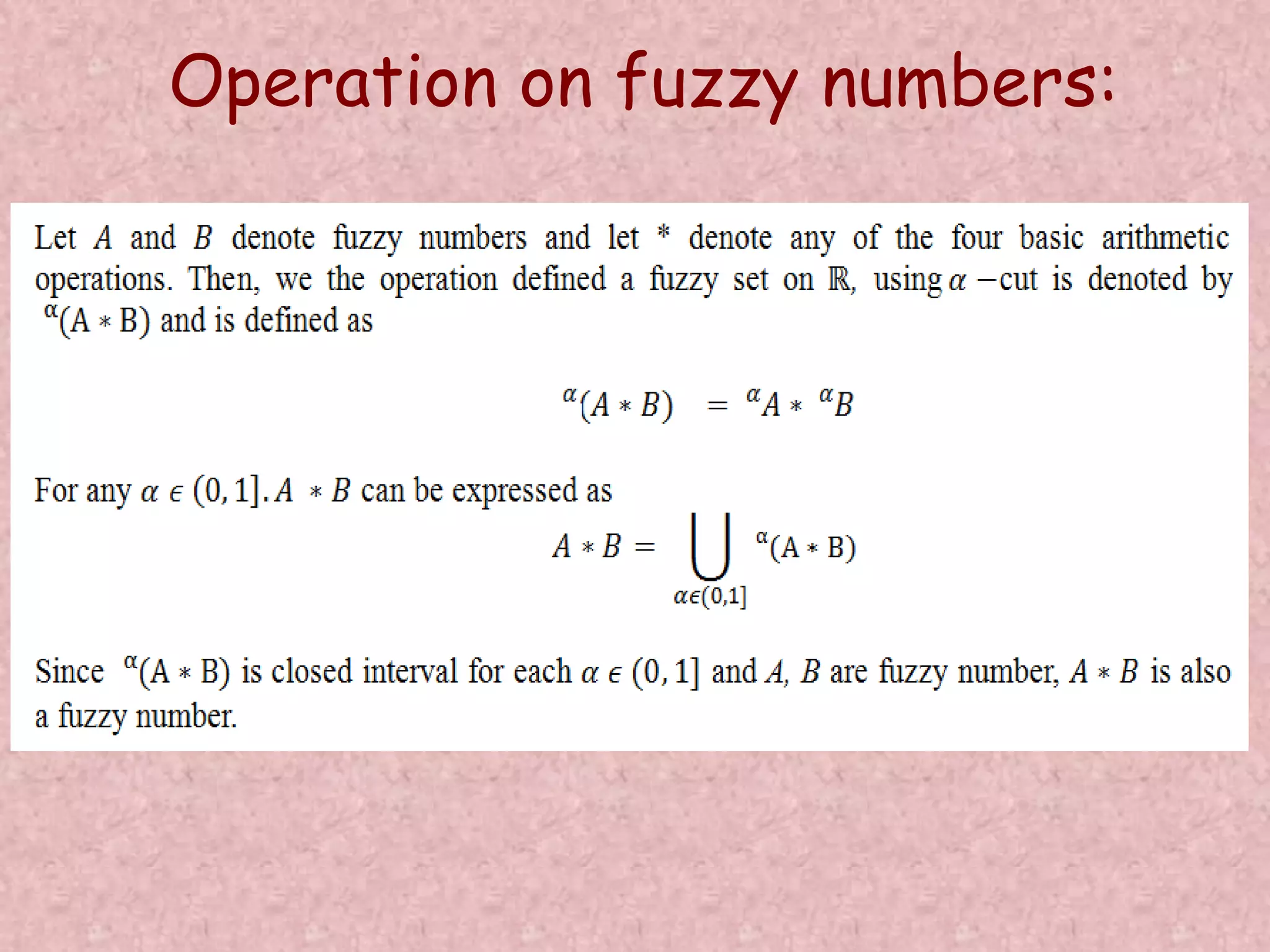
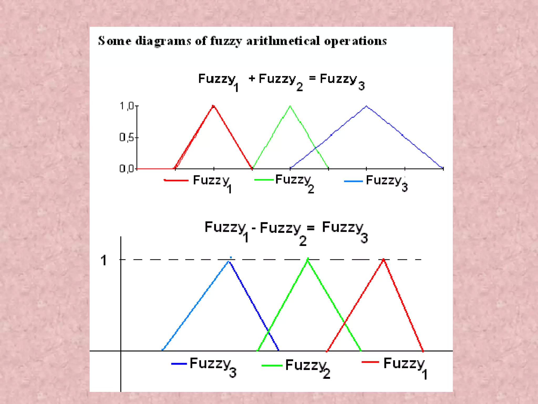
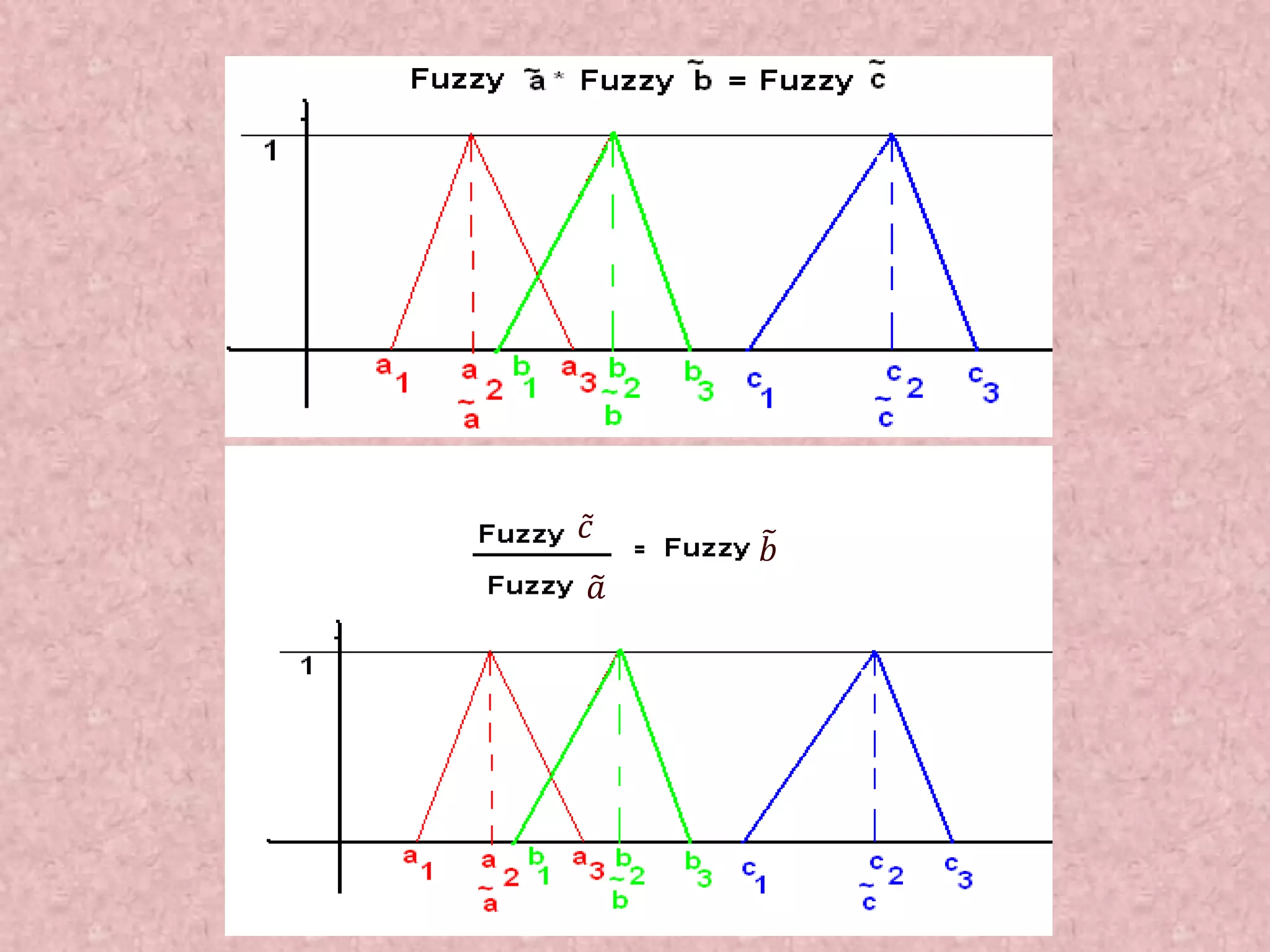
![Fuzzy Arithmetic: Let 𝐴 and 𝐵 are two fuzzy numbers, then on taking alpha-cut we get, 𝐴 𝛼 = 𝐴, 𝐴 and 𝐵 𝛼 = 𝐵, 𝐵 Then, 𝑖 𝐴 𝛼 + 𝐵 𝛼 = [𝐴 + 𝐵, 𝐴 + 𝐵] 𝑖𝑖 𝐴 𝛼 − 𝐵 𝛼 = [𝐴 − 𝐵, 𝐴 − 𝐵] 𝑖𝑖𝑖 𝐴 𝛼. 𝐵 𝛼 = [min( 𝐴 . 𝐵, 𝐴 . 𝐵, 𝐴 . 𝐵, 𝐴 . 𝐵), max ( 𝐴. 𝐵, 𝐴 . 𝐵, 𝐴 . 𝐵, 𝐴. 𝐵)] 𝑖𝑣 𝐴 𝛼/ 𝐵 𝛼 = 𝐴 𝛼. 1/𝐵 𝛼](https://image.slidesharecdn.com/optimizationusingsoftcomputing-171208092056/75/Optimization-using-soft-computing-35-2048.jpg)
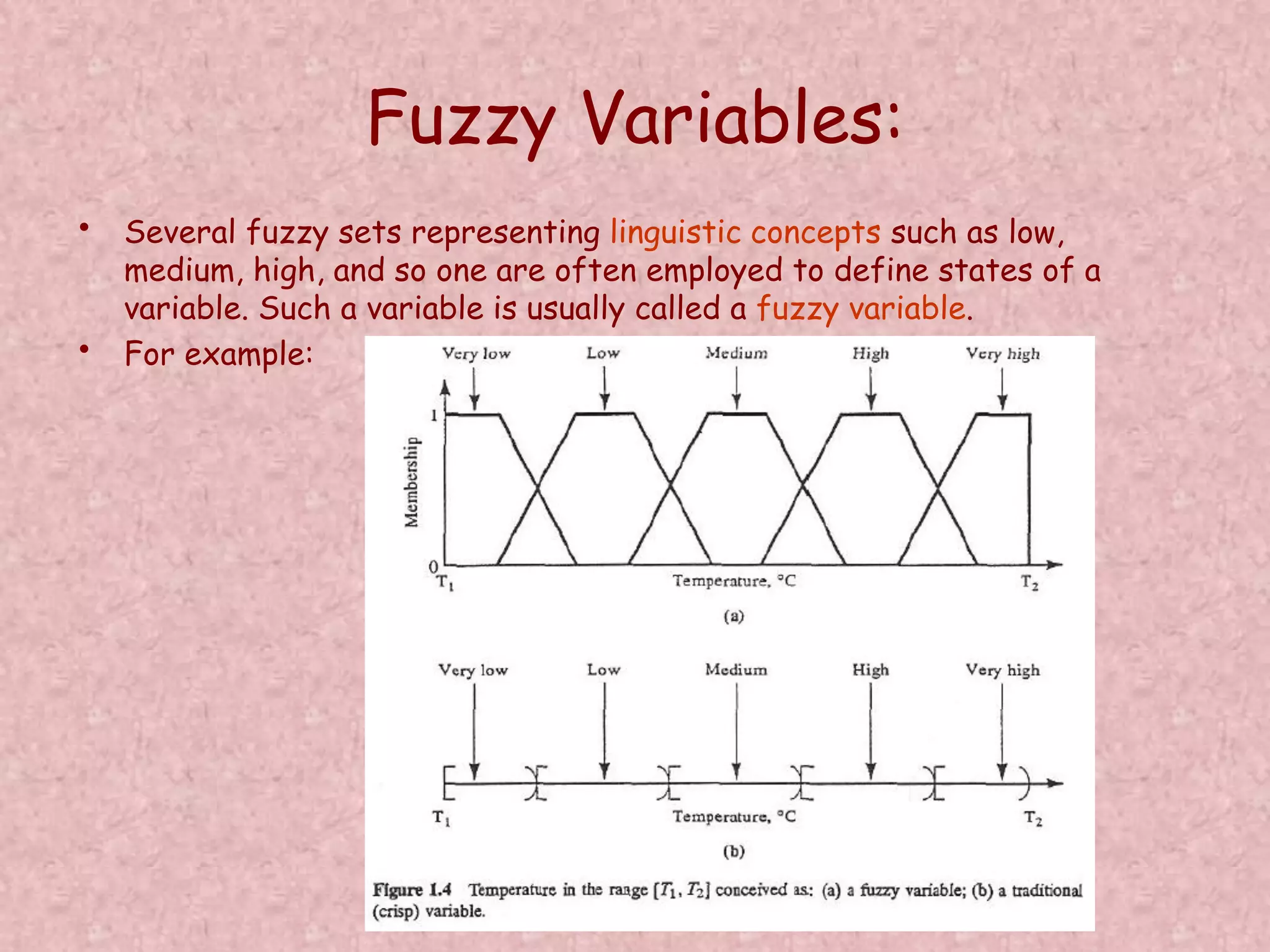
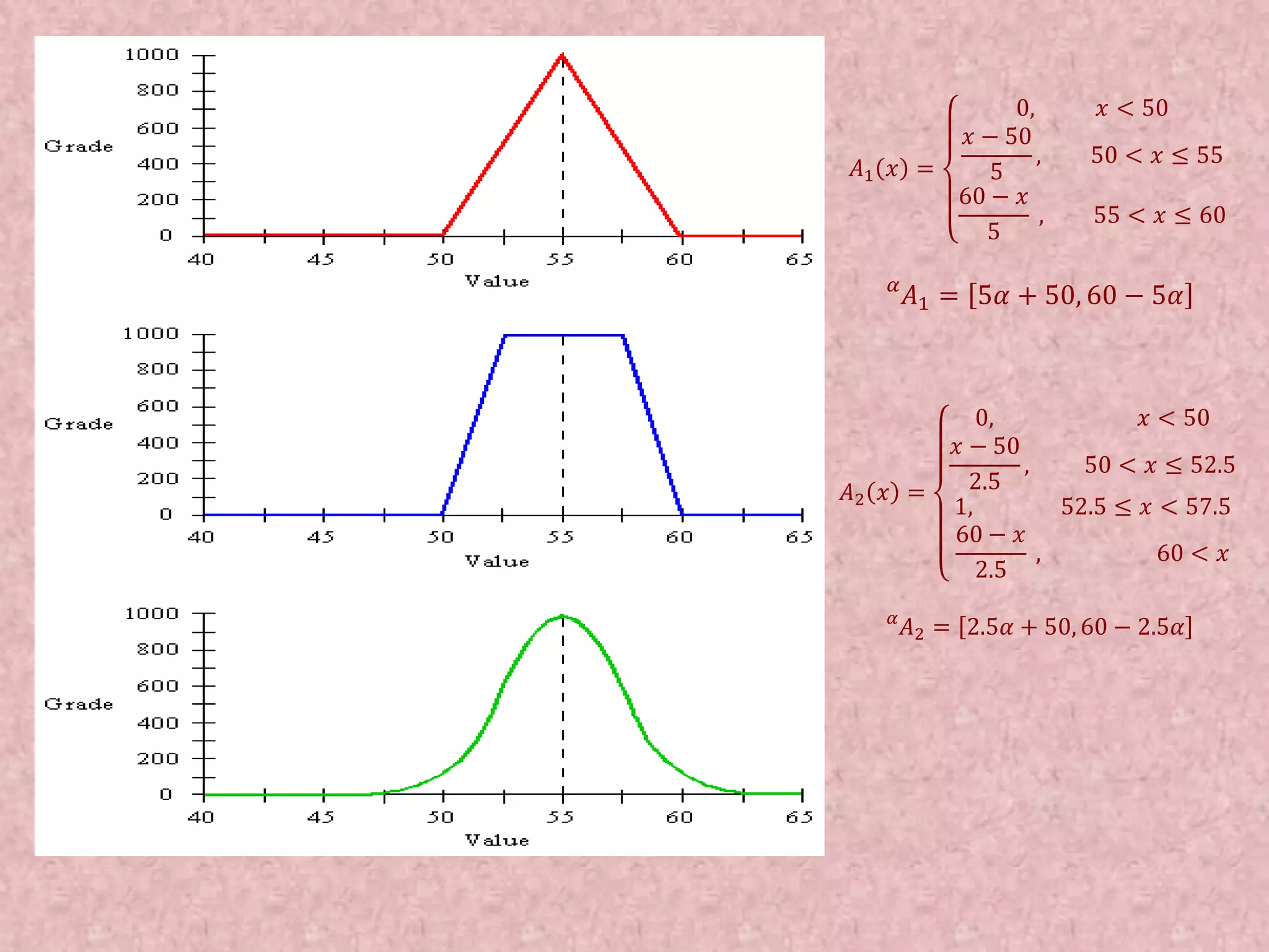
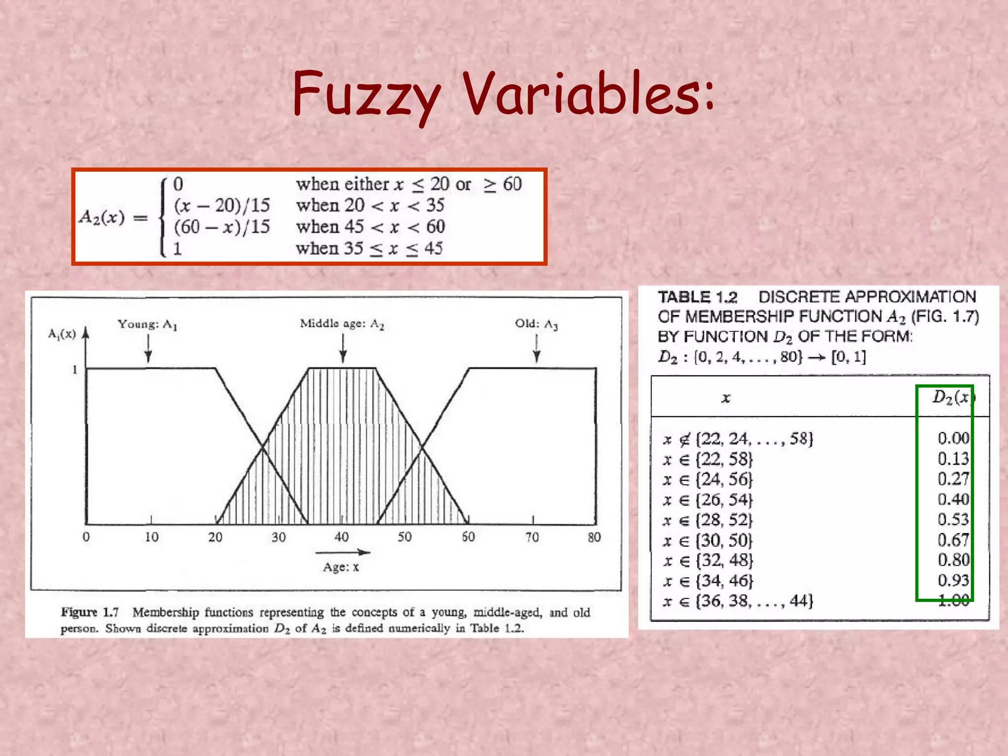
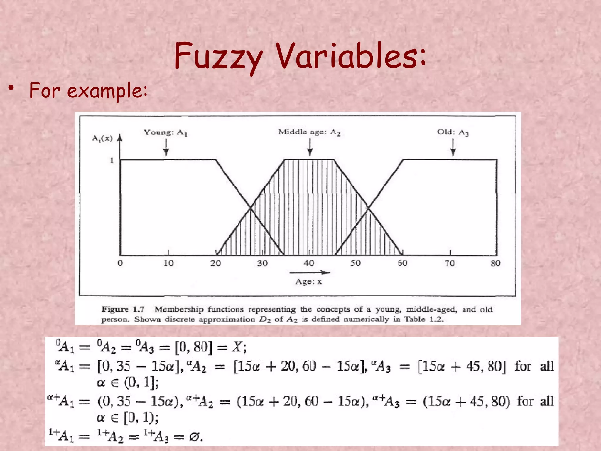
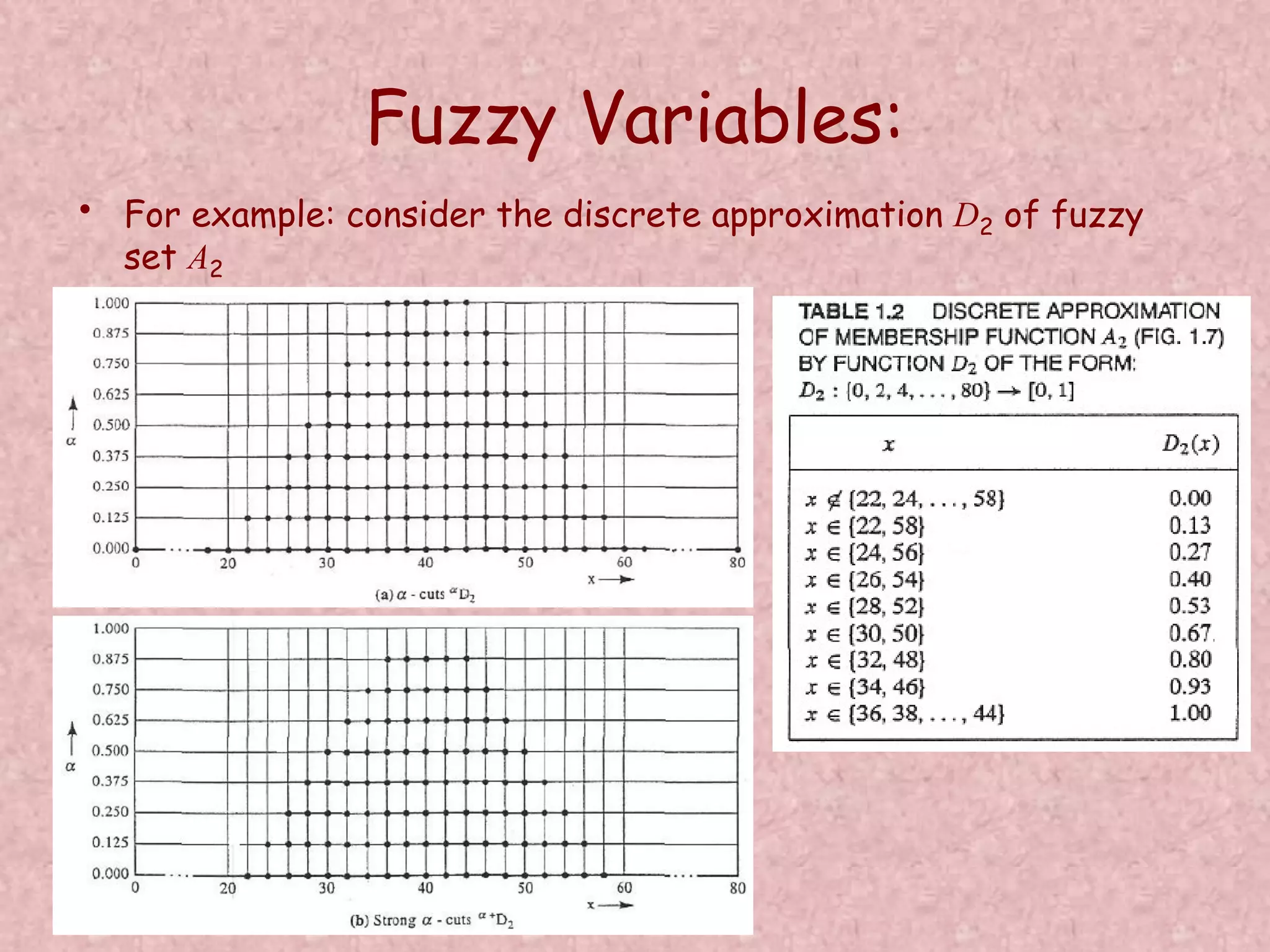
![Fuzzy Variables: • Consider three fuzzy sets that represent the concepts of a young, middle-aged, and old person. The membership functions are defined on the interval [0,80] as follows: Find line passing through (x,y) and (20,1): 1/(35-20) = y/(35-x)](https://image.slidesharecdn.com/optimizationusingsoftcomputing-171208092056/75/Optimization-using-soft-computing-39-2048.jpg)


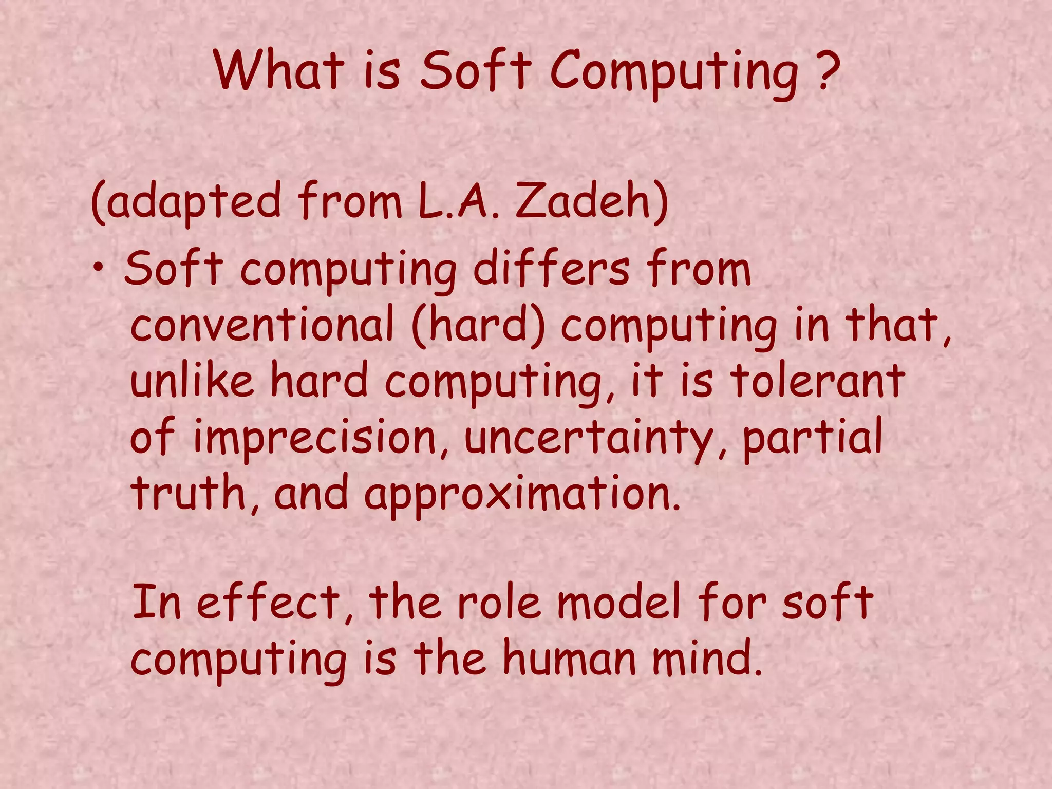
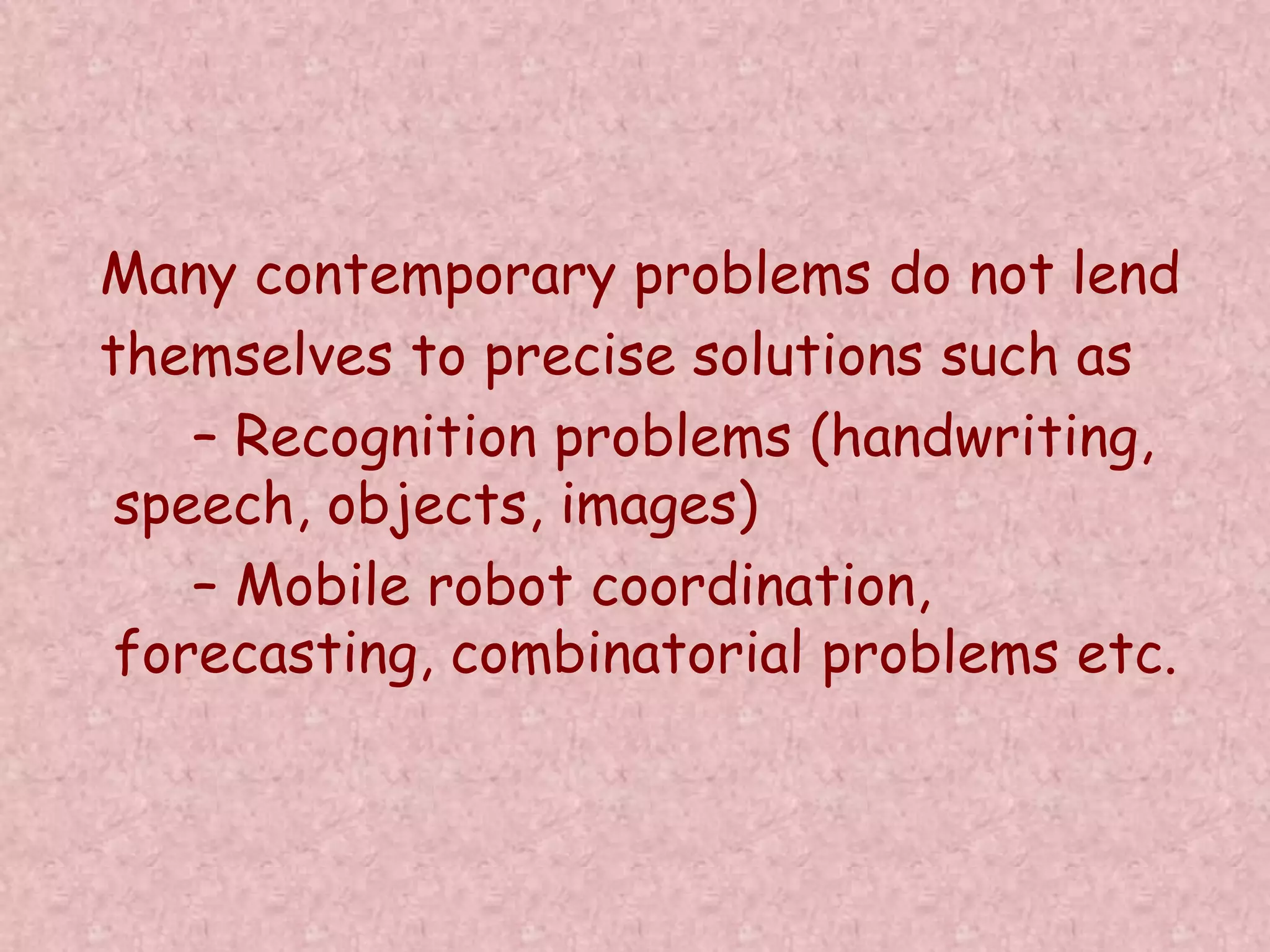
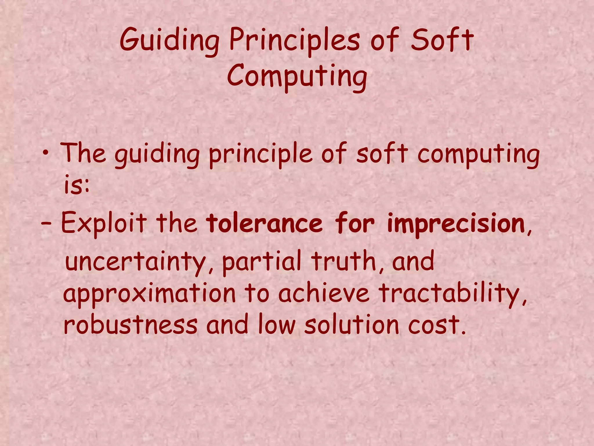
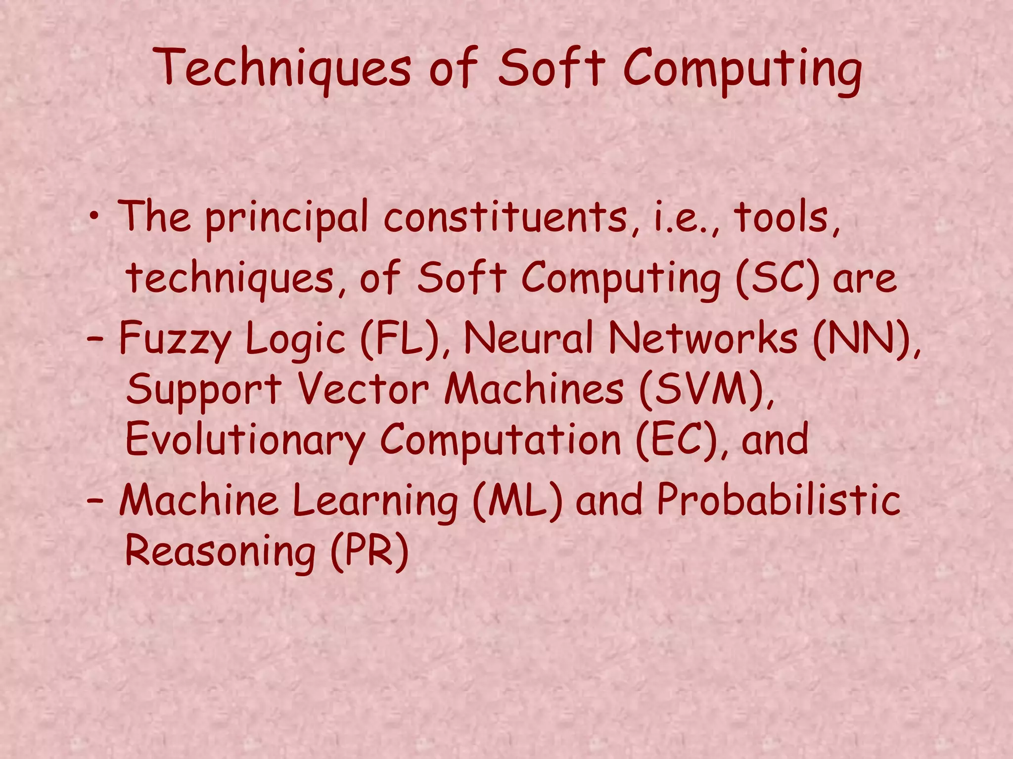
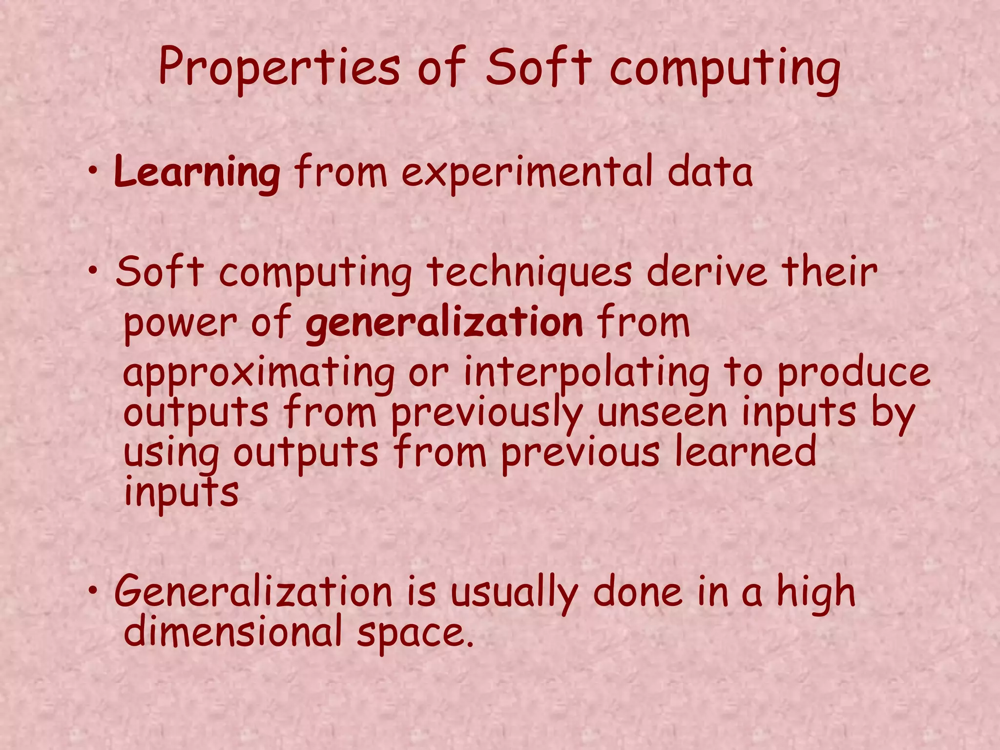
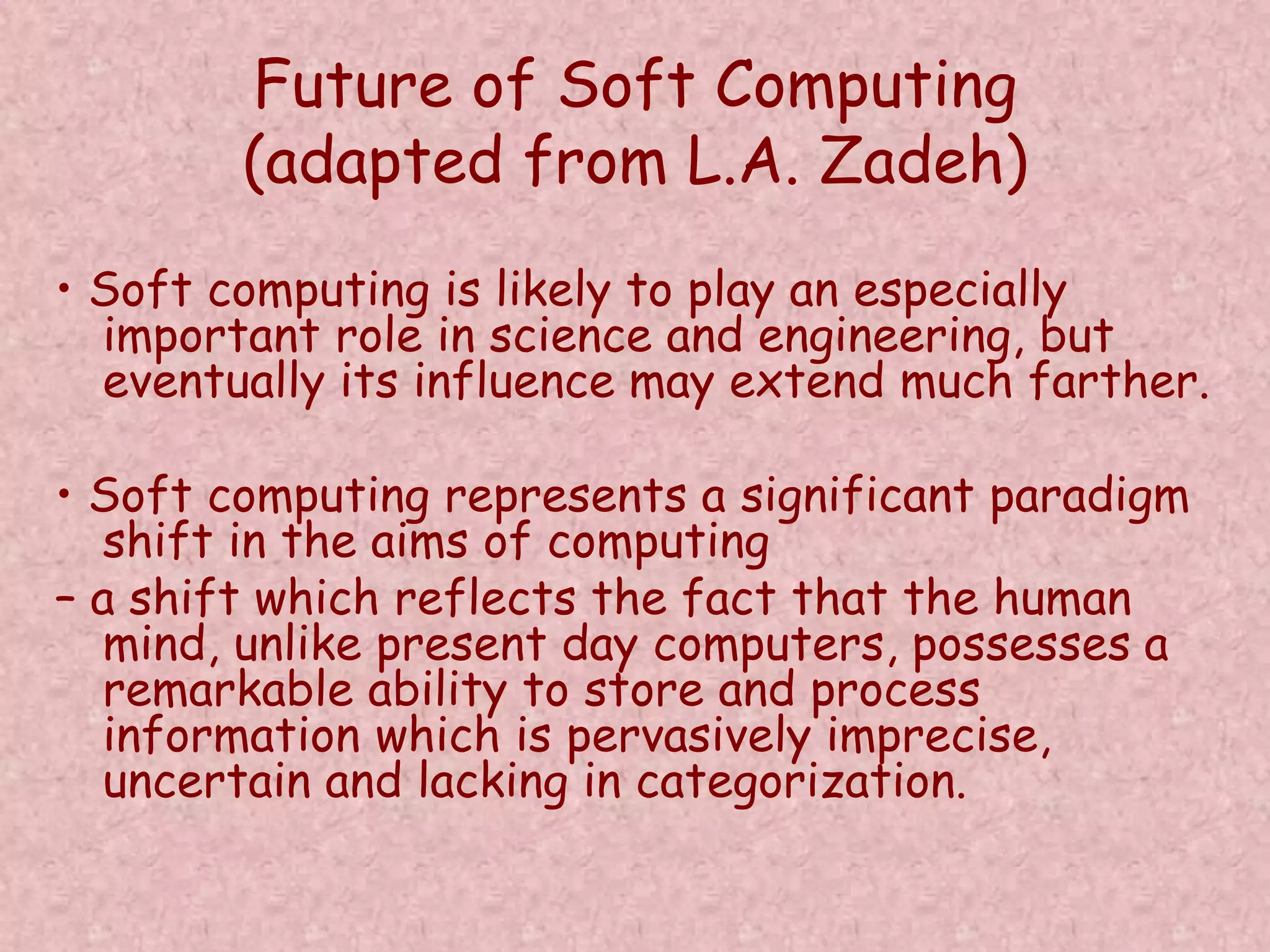
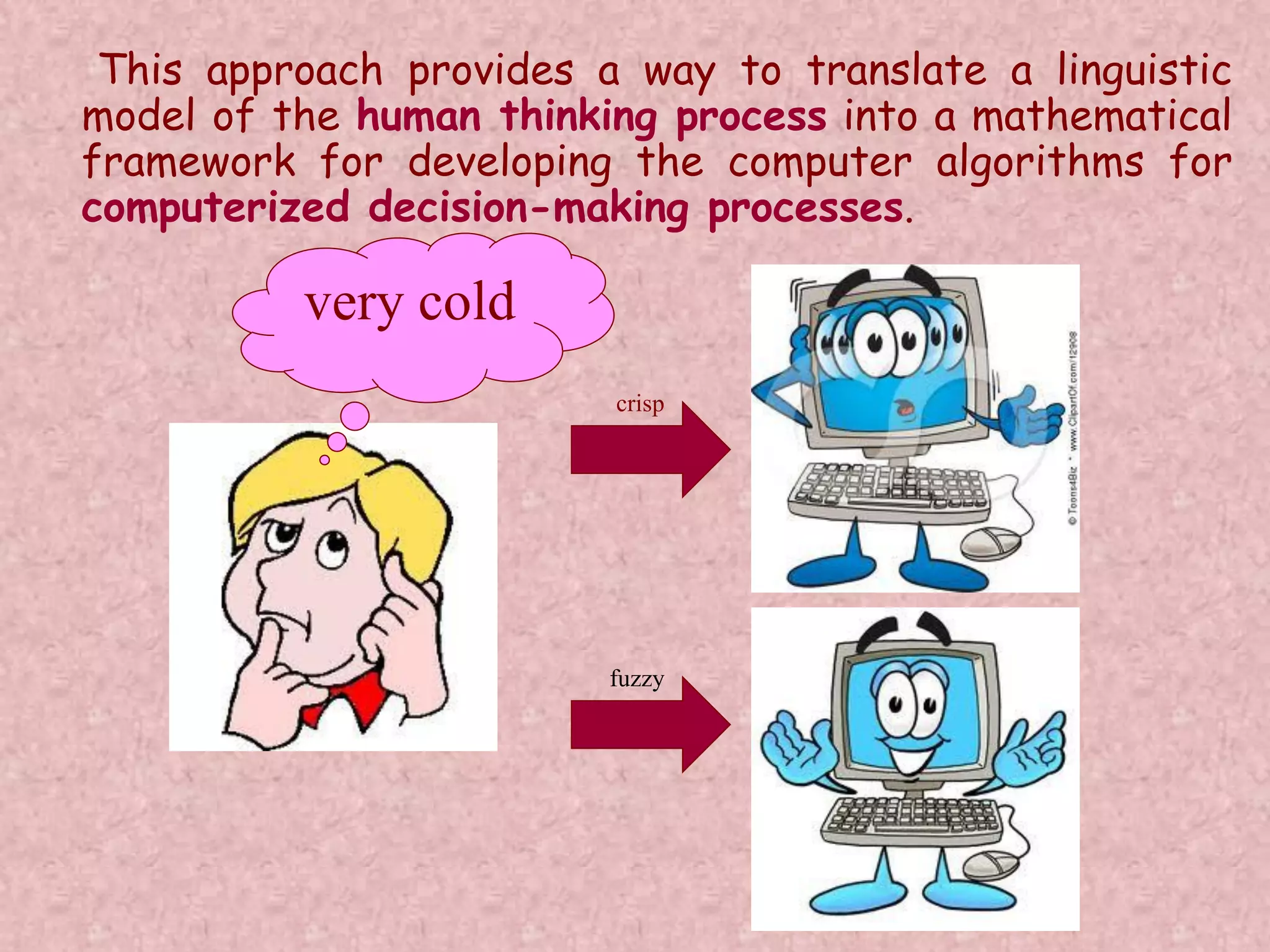
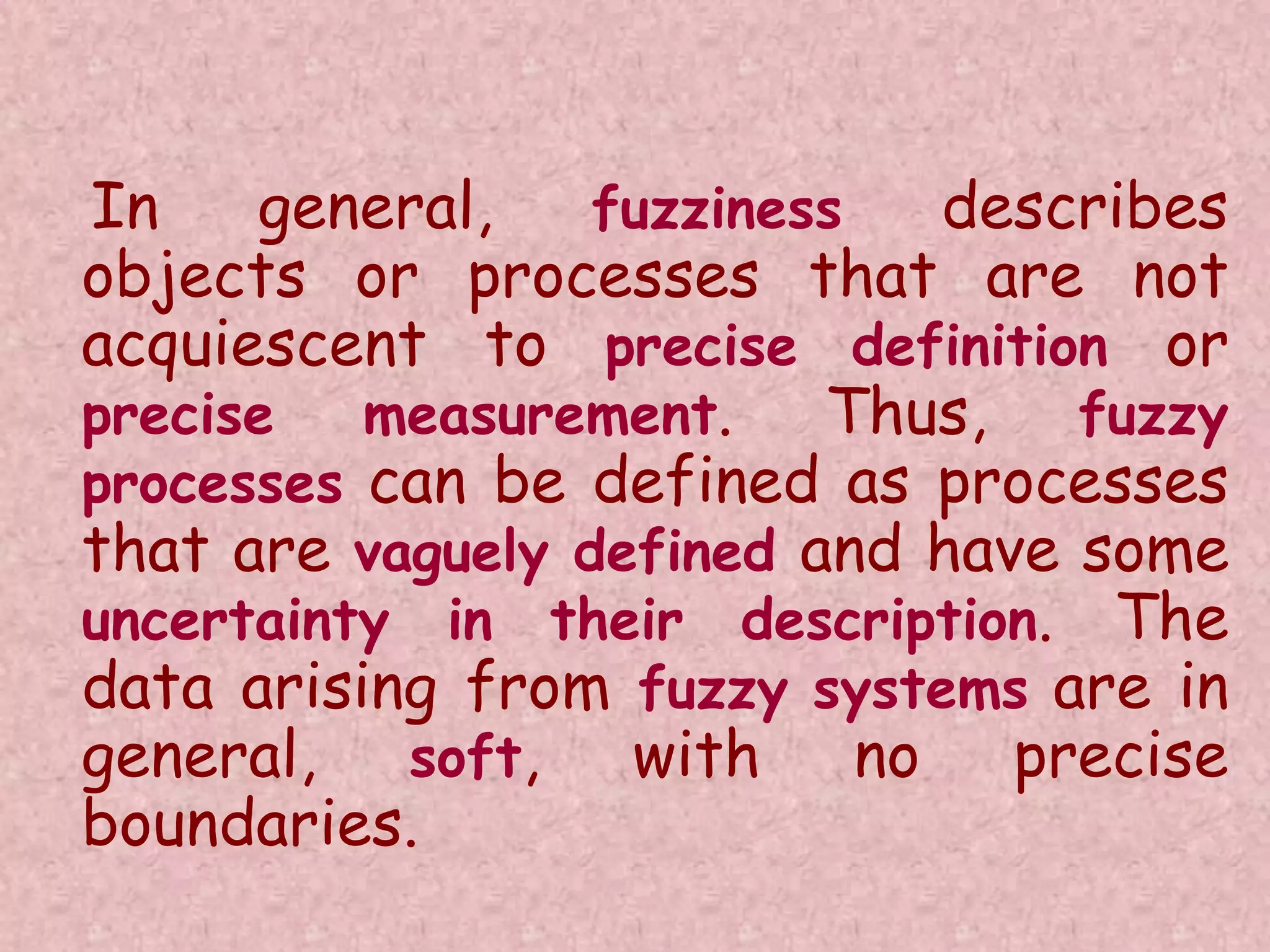
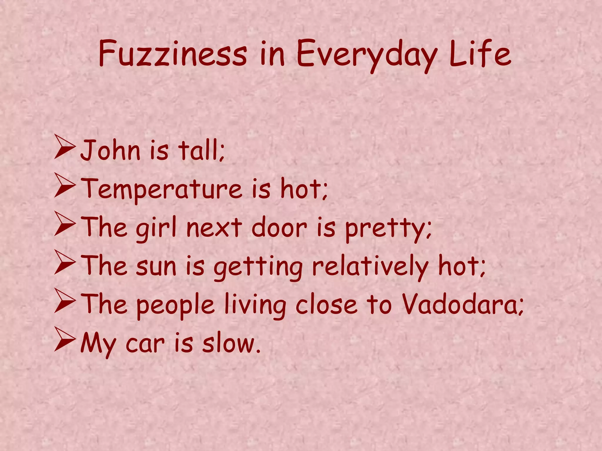
This document discusses soft computing and fuzzy sets. It begins by defining soft computing as being tolerant of imprecision and focusing on approximation rather than precise outputs. Fuzzy sets are introduced as a tool of soft computing that allow for graded membership in sets rather than binary membership. Key concepts regarding fuzzy sets are explained, including fuzzy logic operations, fuzzy numbers, and fuzzy variables. Linear programming problems are discussed and how they can be modeled as fuzzy linear programming problems to account for imprecision in the coefficients and constraints.