Novel DV-Hop algorithm-based machines learning technics for node localization in range-free wireless sensor networks

Novel DV-Hop algorithm-based machines learning technics for node localization in range-free wireless sensor networks

• 1.
  International Journal ofInformatics and Communication Technology (IJ-ICT) Vol. 12, No. 2, August 2023, pp. 140~149 ISSN: 2252-8776, DOI: 10.11591/ijict.v12i2.pp140-149  140 Journal homepage: http://ijict.iaescore.com Novel DV-Hop algorithm-based machines learning technics for node localization in range-free wireless sensor networks Oumaima Liouane1,3 , Smain Femmam2,3 , Toufik Bakir4 , Abdessalem Ben Abdelali1 1 Laboratory of Electronics and Microelectronics (EμE), Faculty of Sciences of Monastir, University of Monastir, Monastir, Tunisia 2 Department of Networks and Communications, Haute-Alsace University, Mulhouse, France 3 EPF Engineering School, Paris-Cachan, France 4 Laboratory ImViA EA 7535, Université Bourgogne, Dijon, France Article Info ABSTRACT Article history: Received Apr 30, 2022 Revised Jul 23, 2022 Accepted Aug 17, 2022 Localization is a critical concern in many wireless sensor network (WSN) applications. Furthermore, correct information regarding the geographic placements of nodes (sensors) is critical for making the collected data valuable and relevant. Because of their benefits, such as simplicity and acceptable accuracy, the based connectivity algorithms attempt to localize multi-hop WSN. However, due to environmental factors, the precision of localisation may be rather low. This publication describes an extreme learning machine (ELM) technique for minimizing localization error in range-free WSN. In this paper, we propose a Cascade-ELM to increase localization accuracy in range-free WSNs. We tested the proposed approaches in a variety of multi-hop WSN scenarios. Our research focused on an isotropic and irregular environment. The simulation results show that the proposed Cascade-ELM algorithm considerably improves localization accuracy when compared to previous algorithms derived from smart computing approaches. When compared to previous work, isotropic environments show improved localization results. Keywords: Deep extreme learning machine Irregularity Localization Machine learning Range free Wireless sensors network This is an open access article under the CC BY-SA license. Corresponding Author: Oumaima Liouane Laboratory of Electronics and Microelectronics (EμE), Faculty of Sciences of Monastir University of Monastir Monastir, Tunisia Email: Oumaima_Liouane@etu.u-bourgogne.fr 1. INTRODUCTION Recent applications of wireless sensor networks (WSN) show one of the most recent developments in wireless communication and industry 4.0 technology. The WSN consist of a collection of sensor devices that are both compact and affordable. These intelligent sensors are able to interact with one another through multi- hop transmission so that they may acquire physical data and phenomena from their surroundings. Each individual device is responsible for data collection and transmission over the network architecture, based on the sensing it possesses. In order to make the data that was obtained usable, it is necessary for the sensor nodes that collected the data to have location awareness so that they can determine where the event is taking place. A few examples of applications in the WSN sector include tracking, supervision, and the internet of things security industry. Recent research efforts have been dedicating to investigating the localization challenges in WSN. In the most recent decade, there has been a heightened focus on the application of machine learning techniques (MLT), in WSN. Artificial neural network (ANN), support vector machine (SVM), and deep learning (DL) approach models are utilized in many domains for the purpose of solving classification problems, estimating densities, or identifying processes, respectively. In point of fact, the MLT method was
• 2.
  Int J Inf& Commun Technol ISSN: 2252-8776  Novel DV-Hop algorithm-based machines learning technics for node localization in … (Oumaima Liouane) 141 implemented in a wide variety of WSN setups, including range-based, range-free, isotropic, and anisotropic settings (see Figure 1). In the range-based scenarios, the ANN inputs shown in Figure 2 present some of the physical features of the signals that were received. These include the received signal strength indicator (RSSI), time of arrival (ToA), time difference of arrival (TDoA), and/or angle of arrival (AoA). These ANN- range-based models have excellent performance when it comes to localization, but they require additional hardware equipment. The location of unknown nodes may be inferred using ANN-range-free approaches, which are based on the connection of WSN and the placements of anchors. These techniques do not require any extra devices. The ANN-range-free localization model is applicable to any kind of isotropic WSN, and it provides accuracy that is satisfactory. Recently, ANN, SVM, extreme learning machine (ELM), and DL have been utilized in order to overcome the challenges of localization in WSNs [1]–[5]. For instance, Javadi et al. [4] utilizes the SVM and a variation of it called twin-SVM in order to localize sources in WSN. Research by Hatami et al. [6] believe that the twin-SVM employs the distributed learning method in order to localize the region surrounding the predicted node position throughout the process of localization. The position of the event that has to be found might be assumed to be the position of the node that has an average position inside the sensing region [4], [7]. Regularized ELM-WSN was utilized by [8]–[11] in order to tackle the multi-hop localization problem. The proposed technique is comprised of three stages: sensing learning data through the correlation between the number of hops and the physical distances separating known and unknown nodes; the trilateration algorithm for the purpose of carrying out the process of localization; and finally [5]. The hybrid localization models that in [12]–[16] the authors described were based on fuzzy logic and the ELM model. In order to achieve the highest possible degree of precision in localisation, the PSO works to mitigate the impact of irregular deployments. A localization approach for large-scale WSNs was reported by [17], [18] using a fast-SVM. The location estimate position of the WSNs is converted into a multiclass problem by the localization method that has been provided, and the binary SVM for localization is utilized in order to find a solution to this problem. The similarity measure is brought to the table by the fast-SVM that has been presented, and the support vectors may be segmented into groups according to the maximal similarity measure [19]. Moreover, Pule et al. [20] proposed combination of the genetic algorithm metaheuristic and the distance vector-hop (DV-Hop) algorithm to compute unknown node coordinates in WSNs. In fact, by using the feasible population region defined by the max-min techniques, the optimization localization process via the genetic algorithm is applied for minimizing the localization errors [21]–[23]. Research by Payal et al. [24] exploit the machine learning ELM to find the appropriate sub-anchor nodes for localization process via the improved DV-Hop localization algorithm. Firstly, the called DV-Hop-ELM upgrades several virtual unknown nodes to sub-anchor nodes via the ELM process. The sub-anchor and real anchor nodes are used together to locate the remaining unknown nodes by the classic DV-Hop algorithm [25]. Recently, Wang et al. [26] proposed the exploitation of the Kernel extreme learning machines based on Hop-count quantization (KELM- HQ) for localization problem in range-free WSNs. The suggested method computes the expected real number of hop-counts between anchors and unknown nodes. For the training phase, the inputs and target outputs of the KELM are respectively the hop-counts number (between anchors and unknown nodes) and the anchors locations. Using the linear-kernel, the proposed method uses the real quantized hop-counts between unknown nodes as the test samples for the localization process in the exploitation phase [27]–[32]. In this work, a novel ANN-range-free model based on Cascade-ELM algorithms for WSN localization is proposed. The Cascade-ELM algorithm is a novel method based on range-free techniques to tackle the localization in WSN. Different scenarios in isotropic environments will be considered to experiment the suggested algorithm and to show the efficacy of the proposed technique. The rest of this paper is presented as follows. Section 2 is dedicated to the review of the state of the art on localization problem in WSN. In sections 3 and 4 we present respectively the basic single hidden layer ELM and the Cascade-ELM and their application for the localization task. Section 5 is dedicated to the analysis of simulation results and the comparison of the proposed ELM architectures performances. Finally, the conclusion and future works are given in section 6. Figure 1. Isotropic WSN deployment (without obstacles) and anisotropic WSN deployment (with obstacles)
• 3.
   ISSN: 2252-8776 IntJ Inf & Commun Technol, Vol. 12, No. 2, August 2023: 140-149 142 Figure 2. Range based deep-ANN localization modes 2. CASCAD-E ELM ALGORITHM DESCRIPTION In WSN, it has been proved that there exists a direct correlation between minimum hop count and the corresponding physical distance. By using the ELM model, the localization of unknown nodes in the WSN can be done by the exploitation of this. In the first learning phase, a beacon packet is broadcasted by each anchor node within the sensing network to inform other nodes about anchors information (ID and Hop-count values). Once a node received this packet the sensor node increments its hop-count. Then, each node computes its cumulative minimum hops counts between them and the anchor nodes. a. Step 1: WSN discovery Like the first step of the basic DV-Hop algorithm called flooding phase, in the first learning phase, a beacon packet is broadcasted by each anchor node within the sensing network to inform other nodes about anchors information (ID and hop-count values). Once a node received this packet the sensor node increments its hop-count. Then, each node computes its cumulative minimum hops counts between them and the anchor nodes. As a result, the minimum hops accounts between all nodes are given and provide the global hop count matrix HC. The HC matrix is divided into two sub-matrix Hca and Hcn designing the anchors connectivity and the unknown nodes connectivity. Moreover, the anchors connectivity Hca matrix play a reference node for the learning phase then the coordinates Xa of all anchor nodes are known the distances matrix Da of the anchor nodes can be directly calculated. b. Step 2: WSN localization learning phase via the ELM model The 2-dimentionnal WSN is composed by (n) randomly deployed nodes which divided in two groups respectively (na) anchors nodes and (nn) unknown nodes. The global hop counts matrix, the global distance matrix between all nodes and the coordinate matrix of all nodes are represented respectively by HC, D and XY. 𝐻𝐶 = ( [𝐻𝑐𝑎] [𝐻𝑐𝑛] ) ∈ 𝑅(𝑛𝑎+𝑛𝑛)×𝑛𝑎 , 𝐷 = ( [𝐷𝑎] [𝐷𝑛] ) ∈ 𝑅(𝑛𝑎+𝑛𝑛)×𝑛𝑎 , 𝑋𝑌 = ( [𝑋𝑎] [𝑋𝑛] ) ∈ 𝑅(𝑛𝑎+𝑛𝑛)×2 − Step 2.1: the first layer of the ELM interpretation We suppose that the relation between hop account matrix HC and the distance matrix D can be expressed by the machine learning process via the ELM Model as shown by Figure 3. Figure 3. The first ELM learning phase The hidden layer matrix can be expressed by: 𝐻 = [ 𝑔(𝐻𝐶1𝑊1 + 𝑏1) 𝐿 𝑔(𝐻𝐶1𝑊 𝑧 + 𝑏𝑧) 𝑀 𝑂 𝑀 𝑔(𝐻𝐶𝑛𝑎+𝑛𝑛𝑊1 + 𝑏1) 𝐿 𝑔(𝐻𝐶𝑛𝑎+𝑛𝑛𝑊 𝑧 + 𝑏𝑧) ] (1)
• 4.
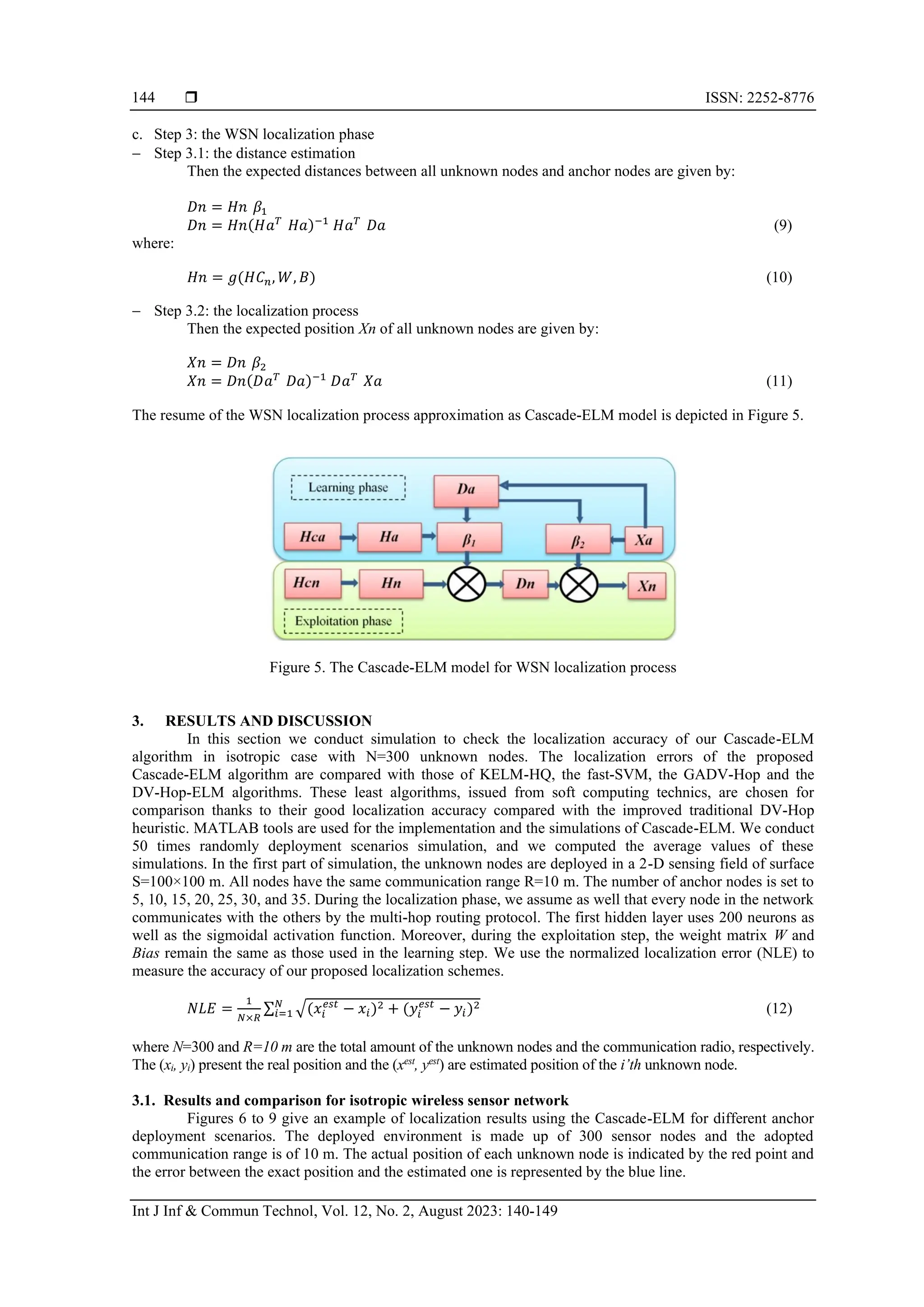
  Int J Inf& Commun Technol ISSN: 2252-8776  Novel DV-Hop algorithm-based machines learning technics for node localization in … (Oumaima Liouane) 143 𝐻 = ( [𝑔(𝐻𝑐𝑎, 𝑊, 𝐵)] [𝑔(𝐻𝑐𝑛, 𝑊, 𝐵)] ) = ( [𝐻𝑎] [𝐻𝑛] ) with 𝐻 ∈ 𝑅(𝑛𝑎+𝑛𝑛)×𝑧 , 𝛽1 ∈ 𝑅𝑧×𝑛𝑎 and 𝐷 ∈ 𝑅(𝑛𝑎+𝑛𝑛)×𝑛𝑎 (2) where g represents the sigmoid activation function. According to the ELM theory, the output layer is given by the least square method: 𝐻 ⋅ 𝛽1 = 𝐷 ⇒ ( [𝐻𝑎] [𝐻𝑛] ) ⋅ 𝛽1 = ( [𝐷𝑎] [𝐷𝑛] ) ⇒ { [𝐻𝑎] ⋅ 𝛽1 = [𝐷𝑎] ⇒ 𝑙𝑒𝑟𝑎𝑛𝑖𝑛𝑔 𝑝ℎ𝑎𝑠𝑒 [𝐻𝑛] ⋅ 𝛽1 = [𝐷𝑛] ⇒ exp𝑙𝑜𝑖𝑡𝑎𝑡𝑖𝑜𝑛 𝑝ℎ𝑎𝑠𝑒 (3) where 𝛽1 represent the output wheigt matrix of the ELM model and can be calculated in the learning phase via the least square optimization method: 𝛽1 = (𝐻𝑎𝑇 𝐻𝑎)−1 𝐻𝑎𝑇 𝐷𝑎 (4) where: 𝐻𝑎 = 𝑔(𝐻𝐶𝑎, 𝑊, 𝐵) (5) The reduced number of the anchor nodes for the training phase introduces the problem of underfitting or overfitting. Then to reduce these problems and ameliorate the generalization error of the localization process via ELM, we use the regularization factor “α” for the output weight 𝛽1 estimation. The “α” parameter controls how much we adjusting the weights of the ELM with respect the generalization error in the exploitation phase. Then the regularized ELM gives the 𝛽1 equal to: 𝛽1 = (𝐻𝑎𝑇 𝐻𝑎 + 𝛼 𝐼𝑑)−1 𝐻𝑎𝑇 𝐷𝑎 (6) where Id denotes (z×z) identity matrix. − Step 2.2: the second layer of the ELM interpretation Moreover, we suppose that the relation between distance matrix D and the coordinate XY of all nodes can be computed by ELM model, in Figure 4 we present the Cascade-ELM learning phase model and this can be calculated in the second learning phase via the least square optimization method: 𝐷 𝛽2 = 𝑋𝑌 ⇒ ( [𝐷𝑎] [𝐷𝑛] ) ⋅ 𝛽2 = ( [𝑋𝑎] [𝑋𝑛] ) ⇒ { [𝐷𝑎] ⋅ 𝛽2 = [𝑋𝑎] ⇒ 𝑙𝑒𝑟𝑎𝑛𝑖𝑛𝑔 𝑝ℎ𝑎𝑠𝑒 [𝐷𝑛] ⋅ 𝛽2 = [𝑋𝑛] ⇒ exp𝑙𝑜𝑖𝑡𝑎𝑡𝑖𝑜𝑛 𝑝ℎ𝑎𝑠𝑒 (7) where 𝛽2 𝑅𝑛𝑎×2 represent the output weight matrix of the second hidden layer and can be calculated via the ELM model: 𝛽2 = (𝐷𝑎𝑇 𝐷𝑎)−1 𝐷𝑎𝑇 𝑋𝑎 (8) Figure 4. The Cascade-ELM learning phase
• 5.
   ISSN: 2252-8776 IntJ Inf & Commun Technol, Vol. 12, No. 2, August 2023: 140-149 144 c. Step 3: the WSN localization phase − Step 3.1: the distance estimation Then the expected distances between all unknown nodes and anchor nodes are given by: 𝐷𝑛 = 𝐻𝑛 𝛽1 𝐷𝑛 = 𝐻𝑛(𝐻𝑎𝑇 𝐻𝑎)−1 𝐻𝑎𝑇 𝐷𝑎 (9) where: 𝐻𝑛 = 𝑔(𝐻𝐶𝑛, 𝑊, 𝐵) (10) − Step 3.2: the localization process Then the expected position Xn of all unknown nodes are given by: 𝑋𝑛 = 𝐷𝑛 𝛽2 𝑋𝑛 = 𝐷𝑛(𝐷𝑎𝑇 𝐷𝑎)−1 𝐷𝑎𝑇 𝑋𝑎 (11) The resume of the WSN localization process approximation as Cascade-ELM model is depicted in Figure 5. Figure 5. The Cascade-ELM model for WSN localization process 3. RESULTS AND DISCUSSION In this section we conduct simulation to check the localization accuracy of our Cascade-ELM algorithm in isotropic case with N=300 unknown nodes. The localization errors of the proposed Cascade-ELM algorithm are compared with those of KELM-HQ, the fast-SVM, the GADV-Hop and the DV-Hop-ELM algorithms. These least algorithms, issued from soft computing technics, are chosen for comparison thanks to their good localization accuracy compared with the improved traditional DV-Hop heuristic. MATLAB tools are used for the implementation and the simulations of Cascade-ELM. We conduct 50 times randomly deployment scenarios simulation, and we computed the average values of these simulations. In the first part of simulation, the unknown nodes are deployed in a 2-D sensing field of surface S=100×100 m. All nodes have the same communication range R=10 m. The number of anchor nodes is set to 5, 10, 15, 20, 25, 30, and 35. During the localization phase, we assume as well that every node in the network communicates with the others by the multi-hop routing protocol. The first hidden layer uses 200 neurons as well as the sigmoidal activation function. Moreover, during the exploitation step, the weight matrix W and Bias remain the same as those used in the learning step. We use the normalized localization error (NLE) to measure the accuracy of our proposed localization schemes. 𝑁𝐿𝐸 = 1 𝑁×𝑅 ∑ √(𝑥𝑖 𝑒𝑠𝑡 − 𝑥𝑖)2 + (𝑦𝑖 𝑒𝑠𝑡 − 𝑦𝑖)2 𝑁 𝑖=1 (12) where N=300 and R=10 m are the total amount of the unknown nodes and the communication radio, respectively. The (xi, yi) present the real position and the (xest , yest ) are estimated position of the i’th unknown node. 3.1. Results and comparison for isotropic wireless sensor network Figures 6 to 9 give an example of localization results using the Cascade-ELM for different anchor deployment scenarios. The deployed environment is made up of 300 sensor nodes and the adopted communication range is of 10 m. The actual position of each unknown node is indicated by the red point and the error between the exact position and the estimated one is represented by the blue line.
• 6.
  Int J Inf& Commun Technol ISSN: 2252-8776  Novel DV-Hop algorithm-based machines learning technics for node localization in … (Oumaima Liouane) 145 Figure 6. Localization results for 5 and 20 anchors Figure 7. Localization results for 35 and 50 anchors As expected in Figure 8, for the KELM-HQ, the fast-SVM, the GADV- Hop, the DV-Hop-ELM and the Cascade-ELM algorithms, the accuracy of localization is ameliorating as the number of anchor nodes increasing. In fact, the increase of the number of anchors leads to increase the number of reference nodes which improving the information for the training phase. Furthermore, the localization error of the proposed Cascade-ELM algorithm was largely smaller than that of its counterparts. In fact, the proposed Cascade-ELM algorithm accuracy increased over 5%, 25%, 15%, and 10% when compared with KELM-HQ, fast-SVM, GADV-Hop the DV-Hop-ELM respectively. Therefore, boosted by the first layer for real distance estimation between anchors and unknown nodes our Cascade-ELM algorithm outperforms in terms of localization accuracy in comparison with the other four algorithms. Consequently, the expected distance between anchors and unknown node corresponds more to the real distance. Hence, the average positioning error will decrease. Figure 9 and Table 1 show the histogram of repartition errors and the statistical results of localization error with different number of anchors. The results are for 50 simulation runs. Figure 8. Localization results of the Cascade-ELM algorithms for 5-35 anchors
• 7.
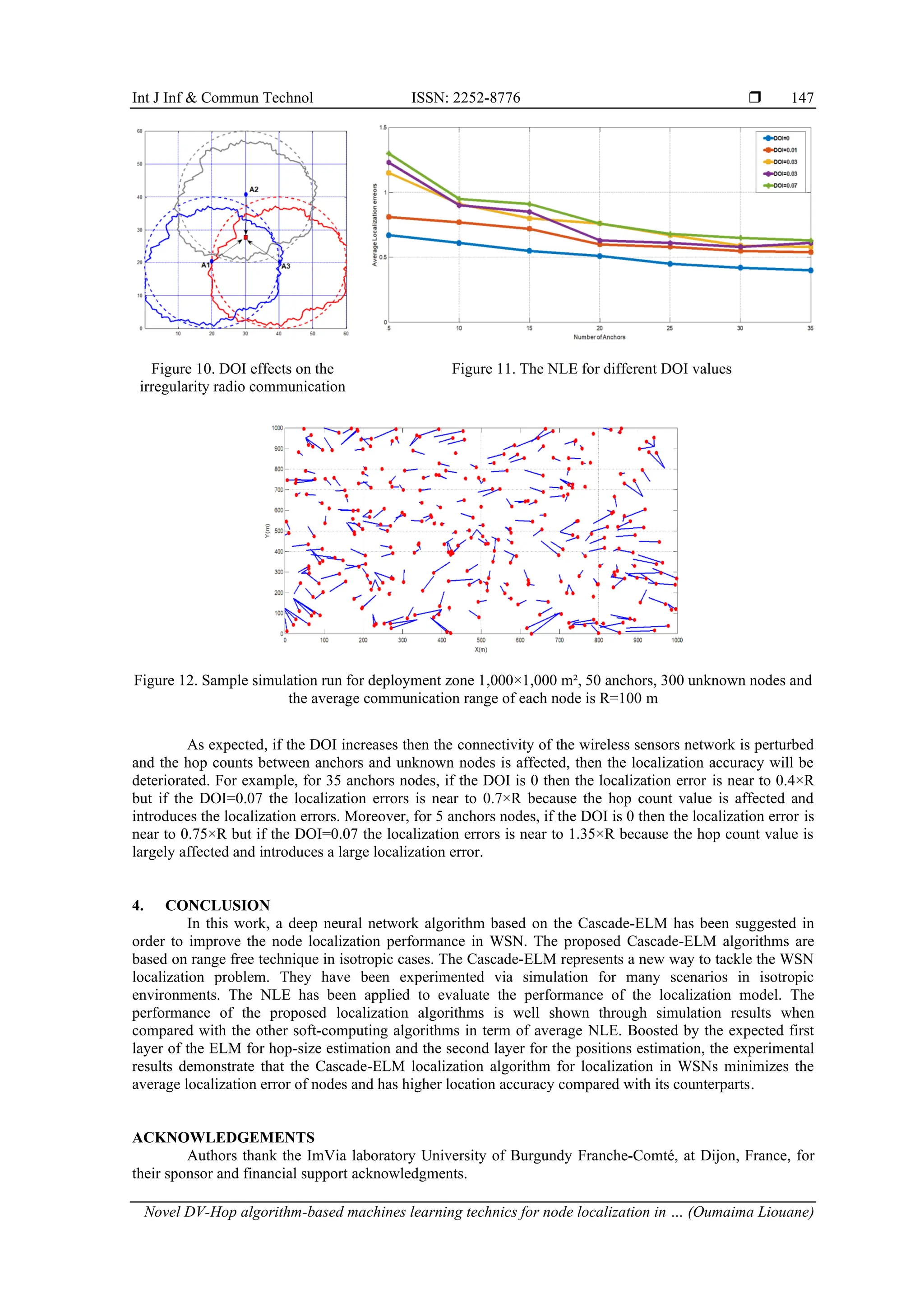
   ISSN: 2252-8776 IntJ Inf & Commun Technol, Vol. 12, No. 2, August 2023: 140-149 146 Figure 9. Histogram of the average localization errors for 50 simulation runs Table 1. Performance results of the Cascade-ELM localization process 5 10 15 20 25 30 35 Min 0.27 0.21 0.23 0.20 0.24 0.20 0.20 Max 1.65 1.61 1.56 1.45 1.3 0.97 0.96 Mean 0.69 0.53 0.51 0.48 0.45 0.42 0.40 Std 0.44 0.38 0.21 0.31 0.24 0.30 0.28 3.2. Degree if irregularity signal effects Practically, in sensor networks the sensed environment is affected by many irregularity effects like the electromagnetic noise and the RSSI variation, thus the radio communication of the radio frequency (RF) sensor nodes will take the form of an irregular elliptic form instead of a standard circle. The impact of radio irregularity on routing protocol can affect the minimum hop counts for localization process in range free WSN. Many researches investigate on the characterization of degree of radio irregularity signal. Indeed, the degree of irregularity (DOI) model draws the maximal variation of radio range per unit degree change within different directions of radio propagation antenna. In the following simulation phase, we exploit the most used DOI model to study the impact of communication irregularity phenomena. In fact, the probability that two nodes can communicate with each other is controlled by a parameter (d). The next model, according to Xiao et al. [13] describes the connectivity probability for two nodes separated by the distance (d) and the ideal communication range R. In this model the probability of the connectivity described by: 𝑃𝑑 = { 1 𝑑 𝑅 < 1 − DOI, 1 2×DOI ( 𝑑 𝑅 − 1) + 1 2 , 1 − DOI ≤ 𝑑 𝑅 ≤ 1 + DOI 0, 𝑑 𝑅 > 1 + DOI (13) As shown in Figure 10, the transmission radio changes with the value of DOI. When DOI=0, the transmission radio R takes the form of an ideal circle. Moreover, as the value of DOI increases as the irregularity of the transmission range increases and affects the number of hops between anchor nodes and the localized nodes. In our simulation, the DOI signal permits to represent the propagation irregularities in WSN localization process. To study the DOI effect on the Cascade-ELM localization process and find the correlation between NLE and the DOI, we implement the localization algorithm with the model of radio range irregularity, and we suppose that sensor nodes have the same transmission range of radius R=100 m. DOI is varied between [0, 0.07]. In the simulation cases, 300 unknown nodes are deployed in a 2-D area of a surface S=1,000×1,000 m with the average communication range R=100 m and the number of anchor nodes is equal to 50. Figure 11 gives the simulation results of the NLE for different anchors deployment and for different values of the DOI. Figure 12 shows an example of localization results given by the proposed Cascade-ELM localization process.
• 8.
  Int J Inf& Commun Technol ISSN: 2252-8776  Novel DV-Hop algorithm-based machines learning technics for node localization in … (Oumaima Liouane) 147 Figure 10. DOI effects on the irregularity radio communication Figure 11. The NLE for different DOI values Figure 12. Sample simulation run for deployment zone 1,000×1,000 m², 50 anchors, 300 unknown nodes and the average communication range of each node is R=100 m As expected, if the DOI increases then the connectivity of the wireless sensors network is perturbed and the hop counts between anchors and unknown nodes is affected, then the localization accuracy will be deteriorated. For example, for 35 anchors nodes, if the DOI is 0 then the localization error is near to 0.4×R but if the DOI=0.07 the localization errors is near to 0.7×R because the hop count value is affected and introduces the localization errors. Moreover, for 5 anchors nodes, if the DOI is 0 then the localization error is near to 0.75×R but if the DOI=0.07 the localization errors is near to 1.35×R because the hop count value is largely affected and introduces a large localization error. 4. CONCLUSION In this work, a deep neural network algorithm based on the Cascade-ELM has been suggested in order to improve the node localization performance in WSN. The proposed Cascade-ELM algorithms are based on range free technique in isotropic cases. The Cascade-ELM represents a new way to tackle the WSN localization problem. They have been experimented via simulation for many scenarios in isotropic environments. The NLE has been applied to evaluate the performance of the localization model. The performance of the proposed localization algorithms is well shown through simulation results when compared with the other soft-computing algorithms in term of average NLE. Boosted by the expected first layer of the ELM for hop-size estimation and the second layer for the positions estimation, the experimental results demonstrate that the Cascade-ELM localization algorithm for localization in WSNs minimizes the average localization error of nodes and has higher location accuracy compared with its counterparts. ACKNOWLEDGEMENTS Authors thank the ImVia laboratory University of Burgundy Franche-Comté, at Dijon, France, for their sponsor and financial support acknowledgments.
• 9.
   ISSN: 2252-8776 IntJ Inf & Commun Technol, Vol. 12, No. 2, August 2023: 140-149 148 REFERENCES [1] D. A. Tran and T. Nguyen, “Localization in wireless sensor networks based on support vector machines,” IEEE Transactions on Parallel and Distributed Systems, vol. 19, no. 7, pp. 981–994, Jul. 2008, doi: 10.1109/TPDS.2007.70800. [2] J. Zheng and A. Dehghani, “Range-free localization in wireless sensor networks with neural network ensembles,” Journal of Sensor and Actuator Networks, vol. 1, no. 3, pp. 254–271, 2012, doi: 10.3390/jsan1030254. [3] P. Cottone, S. Gaglio, G. Lo Re, and M. Ortolani, “A machine learning approach for user localization exploiting connectivity data,” Engineering Applications of Artificial Intelligence, vol. 50, pp. 125–134, Apr. 2016, doi: 10.1016/j.engappai.2015.12.015. [4] S. Javadi, H. Moosaei, and D. Ciuonzo, “Learning wireless sensor networks for source localization,” Sensors, vol. 19, no. 3, pp. 1–17, Feb. 2019, doi: 10.3390/s19030635. [5] W. Zheng, X. Yan, W. Zhao, and C. Qian, “A large-scale multi-hop localization algorithm based on regularized extreme learning for wireless networks,” Sensors, vol. 17, no. 12, pp. 1–18, Dec. 2017, doi: 10.3390/s17122959. [6] A. Hatami, K. Pahlavan, M. Heidari, and F. Akgul, “On RSS and TOA based indoor geolocation - a comparative performance evaluation,” in IEEE Wireless Communications and Networking Conference, 2006. WCNC 2006., 2006, pp. 2267–2272, doi: 10.1109/WCNC.2006.1696648. [7] D. Niculescu and B. Nath, “DV based positioning in ad hoc networks,” Telecommunication Systems, vol. 22, no. 1–4, pp. 267– 280, 2003, doi: 10.1023/A:1023403323460. [8] A. Zhang, Y. Yuan, Q. Wu, S. Zhu, and J. Deng, “Wireless localization based on RSSI fingerprint feature vector,” International Journal of Distributed Sensor Networks, vol. 11, no. 11, pp. 1–7, Nov. 2015, doi: 10.1155/2015/528747. [9] X. Wei, L. Wang, and J. Wan, “A new localization technique based on network TDOA information,” in 2006 6th International Conference on ITS Telecommunications, Jun. 2006, pp. 127–130, doi: 10.1109/ITST.2006.288796. [10] Z. Sahinoglu and I. Guvenc, “Threshold-based TOA estimation for impulse radio UWB systems,” in 2005 IEEE International Conference on Ultra-Wideband, 2005, pp. 420–425, doi: 10.1109/ICU.2005.1570024. [11] H. Dai, W. Ying, and J. Xu, “Multi‐layer neural network for received signal strength‐based indoor localisation,” IET Communications, vol. 10, no. 6, pp. 717–723, Apr. 2016, doi: 10.1049/iet-com.2015.0469. [12] L. Wang, M. J. Er, and S. Zhang, “A kernel extreme learning machines algorithm for node localization in wireless sensor networks,” IEEE Communications Letters, vol. 24, no. 7, pp. 1433–1436, Jul. 2020, doi: 10.1109/LCOMM.2020.2986676. [13] Q. Xiao, B. Xiao, J. Cao, and J. Wang, “Multihop range-free localization in anisotropic wireless sensor networks: a pattern-driven scheme,” IEEE Transactions on Mobile Computing, vol. 9, no. 11, pp. 1592–1607, Nov. 2010, doi: 10.1109/TMC.2010.129. [14] D. Kalpana and P. Ajitha, “An implementation of energy efficient secured routing framework in WSN by honey badger algorithm,” in 2022 International Conference on Industry 4.0 Technology (I4Tech), Sep. 2022, pp. 1–6, doi: 10.1109/I4Tech55392.2022.9952953. [15] A. N. Rao, B. R. Naik, and L. N. Devi, “An efficient coverage and maximization of network lifetime in wireless sensor networks through metaheuristics,” International Journal of Informatics and Communication Technology (IJ-ICT), vol. 10, no. 3, pp. 159– 170, Dec. 2021, doi: 10.11591/ijict.v10i3.pp159-170. [16] B. Lonkar and S. Karmore, “Statistical evaluation of power-aware routing protocols for wireless networks,” International Journal of Intelligent Information Technologies, vol. 18, no. 3, pp. 1–14, Sep. 2022, doi: 10.4018/IJIIT.309589. [17] S. Femmam and I. M. Benakila, “A new topology time division beacon construction approach for IEEE802.15.4/ZigBee cluster- tree wireless sensor networks,” in 2016 IEEE 14th Intl Conf on Dependable, Autonomic and Secure Computing, 14th Intl Conf on Pervasive Intelligence and Computing, 2nd Intl Conf on Big Data Intelligence and Computing and Cyber Science and Technology Congress(DASC/PiCom/DataCom/CyberSciTech), Aug. 2016, pp. 856–860, doi: 10.1109/DASC-PICom-DataCom- CyberSciTec.2016.146. [18] A. Chatterjee, “A fletcher-reeves conjugate gradient neural-network-based localization algorithm for wireless sensor networks,” IEEE Transactions on Vehicular Technology, vol. 59, no. 2, pp. 823–830, Feb. 2010, doi: 10.1109/TVT.2009.2035132. [19] G. Sun and W. Guo, “Robust mobile geo-location algorithm based on LS-SVM,” IEEE Transactions on Vehicular Technology, vol. 54, no. 3, pp. 1037–1041, May 2005, doi: 10.1109/TVT.2005.844676. [20] M. Pule, A. Yahya, and J. Chuma, “Wireless sensor networks: A survey on monitoring water quality,” Journal of Applied Research and Technology, vol. 15, no. 6, pp. 562–570, 2017, doi: 10.1016/j.jart.2017.07.004. [21] O. Liouane, S. Femmam, T. Bakir, and A. B. Abdelali, “On-line sequential ELM based localization process for large scale wireless sensors network,” in 2021 International Conference on Control, Automation and Diagnosis (ICCAD), Nov. 2021, pp. 1– 6, doi: 10.1109/ICCAD52417.2021.9638725. [22] X. Chang and X. Luo, “An improved self-localization algorithm for Ad hoc network based on extreme learning machine,” in Proceeding of the 11th World Congress on Intelligent Control and Automation, Jun. 2014, pp. 564–569, doi: 10.1109/WCICA.2014.7052775. [23] B. Peng and L. Li, “An improved localization algorithm based on genetic algorithm in wireless sensor networks,” Cognitive Neurodynamics, vol. 9, no. 2, pp. 249–256, Apr. 2015, doi: 10.1007/s11571-014-9324-y. [24] A. Payal, C. S. Rai, and B. V. R. Reddy, “Analysis of some feedforward artificial neural network training algorithms for developing localization framework in wireless sensor networks,” Wireless Personal Communications, vol. 82, no. 4, pp. 2519– 2536, Jun. 2015, doi: 10.1007/s11277-015-2362-x. [25] F. Zhu and J. Wei, “Localization algorithm for large scale wireless sensor networks based on fast-SVM,” Wireless Personal Communications, vol. 95, no. 3, pp. 1859–1875, Aug. 2017, doi: 10.1007/s11277-016-3665-2. [26] Y. Wang, X. Wang, D. Wang, and D. P. Agrawal, “Range-free localization using expected hop progress in wireless sensor networks,” IEEE Transactions on Parallel and Distributed Systems, vol. 20, no. 10, pp. 1540–1552, Oct. 2009, doi: 10.1109/TPDS.2008.239. [27] J. Wang, X. Zhang, Q. Gao, H. Yue, and H. Wang, “Device-free wireless localization and activity recognition: a deep learning approach,” IEEE Transactions on Vehicular Technology, vol. 66, no. 7, pp. 6258–6267, Jul. 2017, doi: 10.1109/TVT.2016.2635161. [28] S. Phoemphon, C. So-In, and D. T. Niyato, “A hybrid model using fuzzy logic and an extreme learning machine with vector particle swarm optimization for wireless sensor network localization,” Applied Soft Computing, vol. 65, pp. 101–120, Apr. 2018, doi: 10.1016/j.asoc.2018.01.004. [29] G. bin Huang, N. Y. Liang, H. J. Rong, P. Saratchandran, and N. Sundararajan, “On-line sequential extreme learning machine,” in Proceedings of the IASTED International Conference on Computational Intelligence, 2005, pp. 232–237. [30] G.-B. Huang, D. H. Wang, and Y. Lan, “Extreme learning machines: a survey,” International Journal of Machine Learning and Cybernetics, vol. 2, no. 2, pp. 107–122, Jun. 2011, doi: 10.1007/s13042-011-0019-y.
• 10.
  Int J Inf& Commun Technol ISSN: 2252-8776  Novel DV-Hop algorithm-based machines learning technics for node localization in … (Oumaima Liouane) 149 [31] G.-B. Huang, Q.-Y. Zhu, and C.-K. Siew, “Extreme learning machine: theory and applications,” Neurocomputing, vol. 70, no. 1– 3, pp. 489–501, Dec. 2006, doi: 10.1016/j.neucom.2005.12.126. [32] R. Kapoor and S. Sharma, “BMREWSN: design of a hybrid Bio-inspired model for improving the routing performance of energy- aware wireless sensor networks,” in 2022 IEEE 6th Conference on Information and Communication Technology (CICT), Nov. 2022, pp. 1–6, doi: 10.1109/CICT56698.2022.9997975. BIOGRAPHIES OF AUTHORS Oumaima Liouane received Master Degree in embedded system and instrumentation from the High Institute of Informatics and Mathematics of Monastir (ISIMM) and Ph.D. student at the University of Burgundy Franche-Comte, Dijon, France and National Engineering School of Monastir (ENIM), University of Monastir, Tunisia. Her research interests include the wireless sensors network optimization, machine learning tools, and embedded system. She can be contacted at email: liouaneoumay@gmail.com. Smain Femmam is SMIEEE, IEEE-CA-France section, SMSEE, M-Fellow IETI, he is Professor at the University of Haute-Alsace, France. He received the MS and Ph.D. Degrees in Signal Processing and Computers from Versailles University in 1997 and 1999, respectively. His main research area is signal processing, safety of WSNs and wireless communication. He has a strong interest in perception and characterization of WSN signals, optimal filtering, spectral analysis, wavelets and perception-haptics. He can be contacted at email: smain.femmam@uha.fr. Toufik Bakir received his Ph.D. degree in industrial automatics from the University of Claude Bernard Lyon I, Lyon, France, in 2006. He is currently assistant professor at the laboratory ImVia in the University of Burgundy Franche-Comte, Dijon, France. His research interests include WSN optimization, modeling, and control of dynamic systems. He can be contacted at email: toufik.bakir@u-bourgogne.fr. Abdessalem Ben Abdelali received his degree in Electrical Engineering and his DEA in industrial informatics from the National School of Engineering of Sfax (ENIS), Tunisia, respectively, in 2001 and 2002. He received his Ph.D. from ENIS and Burgundy University (BU), France, in 2007. Since 2017 he has been working as Professor in digital embedded electronic at the High Institute of Informatics and Mathematics of Monastir (ISIMM). His current research interests include reconfigurable architectures and hardware deep learning implementation of image and video processing for WSN applications. He can be contacted at email: abdelalienis@yahoo.fr.