New Method for Tuning PID Controllers Using a Symmetric Send-On-Delta Sampling Strategy

New Method for Tuning PID Controllers Using a Symmetric Send-On-Delta Sampling Strategy

• 1.
  A new methodfor tuning PI controllers with symmetric send-on-delta sampling strategy Julio Ariel Romero Pérez n , Roberto Sanchis Llopis Departament d'Enginyeria de Sistemes Industrials i Disseny, Universitat Jaume I, Campus de Riu Sec, Castelló, Spain a r t i c l e i n f o Article history: Received 8 July 2015 Received in revised form 18 December 2015 Accepted 17 May 2016 Available online 10 June 2016 This paper was recommended for publica- tion by Brent Young. Keywords: PID controller Event-based system Tuning method a b s t r a c t In this paper we present a new method for tuning PI controllers with symmetric send-on-delta (SSOD) sampling strategy. First we analyze the conditions that produce oscillations in event based systems considering SSOD sampling strategy. The Describing Function is the tool used to address the problem. Once the conditions for oscillations are established, a new robustness to oscillation performance measure is introduced which entails with the concept of phase margin, one of the most traditional measures of relative stability in closed-loop control systems. Therefore, the application of the proposed robustness measure is easy and intuitive. The method is tested by both simulations and experiments. Additionally, a Java application has been developed to aid in the design according to the results presented in the paper. & 2016 ISA. Published by Elsevier Ltd. All rights reserved. 1. Introduction During the last years many researches have been focused in event based controllers as alternative to the classical time driven control systems. The main goals in the design of these controllers is the reduction of the frequency of measurement needed for control without degrading the closed loop performance. This is a basic requirement for controllers in networked control systems where many devices (sensors, actuators, and controllers) share a communication channel with limited bandwidth. The reduction in the number of transmitted messages improve the network overall behavior, for example avoiding dropouts and delays. The use of wireless communications in control application has also encour- aged the development of event based controllers. In this case the reduction of data transmission imply an important decrease in power consumption, therefore increasing the lifetime of batteries of self-powered remote sensors [1]. In this context several papers have been published where Event-Based PID control algorithms are proposed. These algo- rithms exploit the properties of the PID control while reducing the network traffic between the controller and the sensor using, in most of the cases, a sampling strategy based on the crossing of levels or thresholds (δ) by the control error signal. This strategy is known as Send-On-Delta (SOD), [2], and its effectiveness in controlling and reducing communication load has been widely contrasted [3,4]. One of the first contributions on Event-Based PID control was introduced by Årzén [5] as a way to reduce the use of CPU in embedded control systems without significantly affecting the closed loop performance. To achieve this goal, the sensor is sam- pled periodically but the control algorithm is activated only if the error exceeds a given threshold. In that paper, some main issues in event-based PID control were addressed, such as the error in the calculation of the integral and derivative terms when the time between samples increases. Some further works have been focused on solving the problems raised by Årzén, mainly related with the calculation of the integral error cited above. It should be noted in particular the works of Durand and Marchand [6,7] and Vasyutynskyy and Kabitzsch [8,9]. A very simple variant of SOD in the context of event based PI controllers has recently been proposed by Beschi et al. in [10]: the sampled signal is quantified by a quantity multiple of δ so that the relationship between the input and output of the event-generator is symmetric with respect to the origin. Thus, this strategy is named symmetric send-on-delta (SSOD) sampling. Relevant results in the field of event based PI controller with SSOD sampling have been obtained during the last years. These results include: (1) necessary conditions on system instability and necessary and sufficient conditions on the controller parameters for the existence of equilibrium points without limit cycles for first order processes plus time delay (FOPTD) [10], (2) characterization of equilibrium point for different kinds of systems such as inte- grating processes plus time delay (IPTD), first order processes plus Contents lists available at ScienceDirect journal homepage: www.elsevier.com/locate/isatrans ISA Transactions http://dx.doi.org/10.1016/j.isatra.2016.05.011 0019-0578/& 2016 ISA. Published by Elsevier Ltd. All rights reserved. n Corresponding author. E-mail addresses: romeroj@uji.es (J.A. Romero Pérez), rsanchis@uji.es (R. Sanchis Llopis). ISA Transactions 64 (2016) 161–173
• 2.
  time delay (FOPTD),and second-order processes plus time delay (SOPTD) [11], (3) tuning rules when the system has a FOPTD model [12], (4) auto-tuning method when the system has an integrator [13]. More general results about this kind of systems were pre- sented in [14], where the authors established the conditions for the DC gain of the open loop transfer function which ensured the absence of oscillations, without assuming any specific model structure. The main result presented in this paper is a new method for tuning PI controllers when SSOD is used in the control loop. First we analyze the conditions that produce oscillations in event based systems considering SSOD sampling strategy. Once the conditions for oscillations are established, a new robustness to oscillation performance measure is introduced, which entails with the con- cept of phase margin, one of the most traditional measures of relative stability in closed-loop control systems. Our proposal is based on the describing function (DF) technique, a well-known tool in the area of non-linear control systems. Because the DF is based on the assumption of negligible higher order harmonics in the close-loop system, which may be a strong assumption, a detailed study is presented here about effect of those harmonics in the proposed tuning method. It is worth mentioning that the results presented in this paper are not restricted to specific model structure, instead they can be applied to a wide range of linear processes including dead-time, non-minimum phase and under-damped response. All the theo- retic results have been put together into a Java application to aid in the design of SSOD based PI controllers. The approach was tested by simulations, using an extensive batch of process models, as well as the real application to a laboratory scale process. 2. Problem statement Consider the networked control system shown in Fig. 1, where C(s) and G(s) are the controller and the process transfer functions respectively, yr is the reference signal to be tracked, y is the con- trolled output, and p is the disturbance input. It is supposed that the controller is located near the actuator and the sensor sends measurements of process output y (or more precisely of the tracking error e) to the controller through a communication net- work using the SSOD strategy. The ZOH block keeps in e the last sent value of process output en until a new value is transmitted by the SSOD block. Concerning the network behavior, it is assumed that the delays in packages transmission are either negligible or known and constant with value td. Although this may be considered restrictive for most real applications, there are powerful reasons to justify this assumption. First, most of industrial communication networks are fast enough to fulfill the timing requirements for process control applications where the system dynamics are slow in comparison to networks transmission rates. Second, nowadays a great research effort is being spent to design protocols to sig- nificantly reduce the package's collision, main cause of variable delays in communication networks, [15]. Communication delays are represented by the terms expðÀtdsÞ in Fig. 1. This control scheme was first proposed in [10] considering C(s) a PI controller, so the authors called it SSOD-PI architecture. As commented in the introduction, some guide lines for the con- troller tuning were given in [12] when the process G(s) is a FOPTD model. Our goal in this paper is to design the controller C(s) in order to reach an adequate performance and robustness of the closed-loop system, for processes with known transfer functions G (s) considering not only FOPTD models but also a more wide range of model structures. The objective of the tuning procedure is not only to guarantee stability but also to avoid persistent oscillations or limit cycles that can appear due to the SOD strategy if the controller is not designed properly. Remark: Another possible send on delta scheme, called PI-SSOD in the literature, could also be considered. It consists of assuming that the controller is located near the sensor, and the SSOD policy is applied to the control action (that is sent to the actuator only when it changes more than delta). The drawback of this approach, as demonstrated by [10], is that the simple existence of the inte- grator leads to an oscillatory behavior unless one of the delta thresholds coincide with the exact input needed in steady state to maintain the output in the required setpoint. As this is not a realistic assumption in real applications, the PI-SSOD scheme always produce persistent oscillations, no matter how the con- troller is tuned. The only way to avoid oscillations in that case (see [10]) is to include a dead band in the error signal. That dead band would change the behavior of the original SOD approach and would make the direct application of the proposed describing function analysis not valid. For those reasons the study of the PI- SSOD scheme will be left for future works, and will not be con- sidered in this paper. 3. Describing function based approach In the control scheme presented in Fig. 1 the SSOD block is followed by a ZOH block. Fig. 2 shows the relation between the SSOD input e and the ZOH output e. The small circles over the diagonal dotted line correspond to the values of en that are sent to the ZOH block. A new value en ¼ iδ; iAZ is sent to the ZOH block when e crosses the levels iδ. The ZOH block keeps this value in the output e until a new value en is sent from the SSOD block. Hor- izontal continuous lines crossing the small circles highlight the fact that e keeps its value for variations of 7δ around the iδ levels. In summary, en denote the discrete values that are sent through the network when the error crosses the thresholds. On the other hand, e is a continuous signal that has the form of consecutive steps that changes when a value of en is received. According to the previous analysis, it is clear that the combi- nation of SSOD and ZOH blocks results in a non-linearity. Conse- quently, the system in Fig. 1, can be represented as that in Fig. 3 where the block SSOD_ZOH represents the combination of SSOD and ZOH blocks. Therefore, the original problem of event based controller is transformed to a non-linear control problem that involves a linear system with a nonlinear block. Following [16] it can be proved (see Appendix A) that the describing function of the SSOD_ZOH block in Fig. 3, considering a sinusoidal input of amplitude A is given by the following equation, NðA; δÞ ¼ 2δ πA 1þ ffiffiffiffiffiffiffiffiffiffiffiffiffiffiffiffiffiffiffiffiffiffiffiffiffi 1À m δ A 2 s2 4 þ2 XmÀ 1 k ¼ 1 ffiffiffiffiffiffiffiffiffiffiffiffiffiffiffiffiffiffiffiffiffiffiffi 1À k δ A 2 s 3 5Àjm 2δ2 πA2 ð1Þ where m ¼ A δ # The describing function in Eq. (1) depends on the quotient δ A. According to Fig. 2, the non-linearity output is zero for inputs withFig. 1. Networked control system with SSOD sampling strategy. J.A. Romero Pérez, R. Sanchis Llopis / ISA Transactions 64 (2016) 161–173162
• 3.
  amplitude Aoδ, thusthe quotient δ A is limited to the interval ½0; 1Š and can be considered as a normalized parameter, δA. Under this consideration Eq. (1) can be written as: NðδAÞ ¼ 2δA π 1þ ffiffiffiffiffiffiffiffiffiffiffiffiffiffiffiffiffiffiffiffiffiffiffiffi 1À mδA À Á2 q þ2 XmÀ 1 k ¼ 1 ffiffiffiffiffiffiffiffiffiffiffiffiffiffiffiffiffiffiffiffiffiffi 1À kδA À Á2 q # Àj 2mδ2 A π ð2Þ This DF can be used to analyze the existence of limit cycles in the closed loop system shown in Fig. 3. The condition for the existence of limit cycles is given by the following equation [16]: Golð jωÞ ¼ À 1 NðδAÞ ð3Þ where Golð jωÞ is the open loop transfer function: Golð jωÞ ¼ Cð jωÞGð jωÞexpðÀtdjωÞ ð4Þ Condition (3) corresponds to the intersections of GolðjωÞ and À1=NðδAÞ in the polar plot. The portrait of À1=NðδAÞ, which is shown in Fig. 4, can obtained by evaluating Eq. (2) for δA A½0; 1Š. 4. Tuning SSOD based PI controllers Taking into account the shape of the Nyquist diagrams of usual processes, the most critical point in the plot in order to avoid the intersection between GolðjωÞ and À1=NðδAÞ is the point Àπ 4 Àπ 4j ¼ π ffiffi 2 p 4 expðÀ3π 4 jÞ, shown as point C in Fig. 4. This point is obtained for δA ¼ 1. As it will be shown in the next section, for most of the common types of processes, if the Nyquist plot of Gol ðjωÞ does not encircle that point, then there is no intersection with the DF plot, and hence, there are no oscillations. Based on this simple idea, a new robustness measure is pro- posed to evaluate the robustness of the controlled system with respect to undesired oscillations: the SSOD phase margin, Φm;ssod, i.e. a phase margin to avoid limit cycle. It is defined as the phase that should be added to GolðjωÞ to make the Nyquist plot cross the critical point C, see Fig. 5. To define this specification precisely, let us define a new gain crossover frequency, ωg0 , as the frequency where jGolðjωg0 Þj ¼ π ffiffi 2 p 4 % 1:11. This new gain crossover frequency is different from the usual one, ωg, defined as jGolðjωgÞj ¼ 1. The phase margin to avoid limit cycle is then defined as: Φm;ssod ¼ argðGolð jωg0 ÞÞÀarg À π 4 À π 4 j ¼ argðGolð jωg0 ÞÞþ 3π 4 It should be noted that the final phase margin in the classical sense, that measures robustness to instability, will be somehow near Φm;ssod þπ 4 (or Φm;ssod þ451). However, it is not sufficient to choose a classical phase margin larger than 45° to guarantee the avoidance of the limit cycle as the classical phase margin is defined where the magnitude is 1, and not 1.11, and hence, the Nyquist plot could still intersect the DF plot. The selection of the final phase margin greater than 45°, as proposed by the authors in [17], can be considered a general and intuitive rule of thumb for tuning SSOD based PI controllers, but not an exact method to avoid limit cycles as the one presented here. Based on the definition of phase margin to oscillations ðΦm;ssodÞ, the PI design method described in [18] is proposed to be modified in the following to be adapted to the SSOD sampling scenario. The transfer function of the PI controller is assumed to be CðsÞ ¼ Kp 1þ 1 Tis ¼ Kp þ Ki s ð5Þ where Ki ¼ Kp Ti ð6Þ The objective of the PI controller to be designed is to reach an adequate performance and robustness of the controlled system, taking into account the assumed event based sampling, expressed in the following design specifications: Required phase margin to avoid limit cycle: Φm;ssod;r. The phase margin ðΦm;ssodÞ should be equal to this value ðΦm;ssod ¼ Φm;ssod;rÞ. Fig. 2. Input/output characteristic of the SSOD_ZOH block combination. Fig. 3. Non-linear equivalent system to the control systems with SSOD sampling strategy in Fig. 1. −1.6 −1.4 −1.2 −1 −0.8 −0.6 −1 −0.9 −0.8 −0.7 −0.6 −0.5 −0.4 −0.3 −0.2 −0.1 0 0.1 Real Imaginary C Fig. 4. Polar plot of À1=N. J.A. Romero Pérez, R. Sanchis Llopis / ISA Transactions 64 (2016) 161–173 163
• 4.
  Minimum required gainmargin: γm;r. The gain margin (γm) should be larger than or equal to this value ðγm Zγm;rÞ. Good disturbance rejection: The step disturbance IAE should be as low as possible. 4.1. PI design method The design method can be summarized as a constrained opti- mization approach in which the proposed PI parameters are those that maximize the controller integral gain ðKi ¼ Kp Ti Þ, subject to the following constraints: Φm;ssod ¼ Φm;ssod;r, γm Zγm;r. The maximization of Ki is equivalent to the minimization of the integral of the error (IE) of the step disturbance response, because it is well known that IE ¼ lim t-1 Z t 0 eðτÞdτ ¼ lim s-0 GðsÞ sð1þCðsÞGðsÞÞ ¼ 1 Ki ð7Þ If the phase and gain margins specifications are large enough, then the closed loop response is not too oscillatory, and the IE is similar to the IAE. Therefore, the approach is equivalent to an approximate minimization of the IAE. The key to solve the previous constraint maximization problem straightforwardly is to introduce a tuning parameter that is the relation between the final gain crossover frequency of the process with controller to avoid limit cycles and the controller zero a ¼ ωg0 zi ¼ ωg0 Ti ð8Þ where ωg0 is the frequency where the magnitude of the open loop frequency response of the process plus controller is Golðjωg0 Þ ¼ π ffiffi 2 p 4 % 1:11, i.e. where the phase margin to avoid limit cycle is measured. For a given value of this parameter a, the phase of the controller at the final crossover frequency ωg0 depends only on that value: argðCðjωg0 ÞÞ ¼ arctanðaÞÀ π 2 ¼ Àarctan 1 a ð9Þ Therefore, for a given value of parameter a, the calculation of the controller is automatic, following two steps 1. The final crossover frequency ðωg0 Þ is obtained as the frequency where the phase of the system fulfills the phase margin equation, i.e. where the phase of the system is argðGð jωg0 ÞÞ ¼ À 3π 4 þΦm;ssod;r ÀargðCð jωg0 ÞÞ ¼ Φm;ssod;r À π 4 ÀarctanðaÞ ð10Þ Then, the value of the integral time (Ti) is calculated as Ti ¼ a ωg0 2. The value of Kp is calculated from the condition of magnitude π ffiffi 2 p 4 % 1:11 at the final crossover frequency jCð jωg0 ÞGð jωg0 Þj ¼ π ffiffiffi 2 p 4 - Kp ð11Þ The resulting equation for Kp is: Kp ¼ π ffiffiffi 2 p 4 a jGðjωg0 Þj ffiffiffiffiffiffiffiffiffiffiffiffiffi 1þa2 p ð12Þ In the previous steps, the available frequency response data of the process is used, interpolating, if necessary, between the available points. Once the controller parameters are defined, the final gain margin, γm, can be calculated. The proposed PI design method can be expressed as the fol- lowing optimization problem over a single real parameter, a: max a Ki s:t:Φm;ssod ¼ Φm;ssod;r γm Zγm;r ð13Þ This is a very simple one-dimensional optimization problem in which the search space for parameter a is small and well defined. According to Eq. (9), the phase contribution of argðCðjωg0 ÞÞ, is sig- nificant only in the range 0oao6 as shown in Fig. 6, therefore the optimal value of a is expected to be in that range. Remark: The shape of À 1 NðδAÞ in Fig. 4 is completely defined by δA A½0; 1Š and does not depend on the value of δ. That means that once the controller C(s) is designed to avoid the limit cycle, this condition is fulfilled regardless of the value of the parameter δ. As a result, nor stability neither robustness of the closed loop system in Fig. 1 are affected by the value on δ. The value of δ, however, determines the steady state error because the block ZOH_SSOD in Fig. 1 introduces a dead-zone effect of amplitude δ. Thus, greater values of δ may potentially lead to higher steady state errors. The parameter δ is also related to the event generation rate by an inverse relationship, [12]. Taking this into account, the selection of δ should be a trade-off between the steady state requirements and communication restrictions. Remark: The proposed design approach does not take into account the use of a weighting factor for the proportional term of the reference. This weighting factor bo1 is usually added in the calculation of the proportional part of the control action as up ¼ Kpðb yr ÀyÞ. If the overshoot of the step reference response is too high, an adequate selection of this factor b can reduce it to a lower level. Trial and error can be used to adjust the value of b. If a transfer function model of the process is available, this trial and error can be made in simulations. 5. Validity of the approach The oscillation condition used to define the new phase margin was obtained by the DF method, which is valid only if the linear part of the system in Fig. 3 is filtering enough to neglect the higher Fig. 5. The new robustness measure, Φm;ssod. J.A. Romero Pérez, R. Sanchis Llopis / ISA Transactions 64 (2016) 161–173164
• 5.
  order harmonics inthe input of the non-linearity. The relaxation of this condition could introduce errors in the limit cycle prediction, and might result in undesired oscillation. In this section we study the effect of the higher harmonics in the phase margin for oscil- lation Φm;ssod predicted by de DF. Concretely we analyze the var- iations in the critical point C in Fig. 4 due to these harmonics. Suppose we design the PI that maximize the gain Ki with Φm;ssod ¼ 0. With that controller, the open loop transfer function of the system in Fig. 3 crosses the point C. Let us define ωc as the frequency where GolðjωcÞ ¼ Àπ 4 Àπ 4j. The resulting closed loop oscillation with that controller would be as shown in Fig. 7, which shows the input (e) and output ðeÞ of the non-linearity SSOD_ZOH. The signal e fulfills conditions (14), where To is the period of oscillation and the initial time is considered in the rising edge of e. The frequency of oscillation, ωo ¼ 2π=To, will be closed to ωc, but not exactly that one due to the higher order harmonics effects: e To 4 ¼ 0 ð14aÞ e To 2 ¼ Àδ ð14bÞ The Fourier transform of e is: eðtÞ ¼ 4δ π X1 n ¼ 1;3;5;… 1 n sin nπ 4 cos nwotÀ nπ 4 ð15Þ eðtÞ ¼ 4δ π X1 n ¼ 1;3;5;… 1 n sin nπ 4 real exp Àj nπ 4 þjnwot ð16Þ where wo is the frequency of oscillation. Then, the output of the open loop transfer function Gol(s) is: yðtÞ ¼ 4δ π X1 n ¼ 1;3;5;… 1 n sin nπ 4 real GolðjnwoÞexp Àj nπ 4 þjnwot ð17Þ Fig. 6. argðCð jωg0 ÞÞ as function of the parameter a. Fig. 7. Oscillation in the SSOD PI based systems. Fig. 8. Higher order harmonics contribution to robustness, ΔΦssod. Positive case. Fig. 9. Higher order harmonics contribution to robustness, ΔΦssod. Negative case. J.A. Romero Pérez, R. Sanchis Llopis / ISA Transactions 64 (2016) 161–173 165
• 6.
  Considering yr ¼0,then eðtÞ ¼ ÀyðtÞ, and evaluating e(t) in t ¼ T0=4 and t ¼ T0=2 results in: eðT0=4Þ ¼ À 4δ π X1 n ¼ 1;3;5;… 1 n sin nπ 4 real GolðjnwoÞexp j nπ 4 ð18Þ eðT0=2Þ ¼ 4δ π X1 n ¼ 1;3;5;… 1 n sin nπ 4 real GolðjnwoÞexp Àj nπ 4 ð19Þ Defining RolðnwoÞ ¼ realðGolðjnwoÞÞ; IolðnwoÞ ¼ imagðGolðjnwoÞÞ and using the Euler expressions of the complex exponentials, then Eqs. (18) and (19) can be written as eðT0=4Þ ¼ À 4δ π X1 n ¼ 1;3;5;… 1 n sin nπ 4 RolðnwoÞ cos nπ 4 ÀIolðnwoÞ sin nπ 4 ð20Þ eðT0=2Þ ¼ 4δ π X1 n ¼ 1;3;5;… 1 n sin nπ 4 RolðnwoÞ cos nπ 4 þIolðnwoÞ sin nπ 4 ð21Þ Therefore, the conditions expressed in (14) can be written as À 4δ π X1 n ¼ 1;3;5;… 1 n sin nπ 4 cos nπ 4 RolðnwoÞ þ 4δ π X1 n ¼ 1;3;5;… 1 n sin 2 nπ 4 IolðnwoÞ ¼ 0 ð22Þ 4δ π X1 n ¼ 1;3;5;… 1 n sin nπ 4 cos nπ 4 RolðnwoÞ þ 4δ π X1 n ¼ 1;3;5;… 1 n sin 2 nπ 4 IolðnwoÞ ¼ Àδ ð23Þ which can be reduced to: X1 n ¼ 1;3;5;… 1 n sin nπ 4 cos nπ 4 RolðnwoÞ ¼ À π 8 ð24Þ X1 n ¼ 1;3;5;… 1 n sin 2 nπ 4 IolðnwoÞ ¼ À π 8 ð25Þ The previous equations can be written as: RolðwoÞ ¼ À π 4 À X1 n ¼ 3;5;… 2 n sin nπ 4 cos nπ 4 RolðnwoÞ ð26Þ and IolðwoÞ ¼ À π 4 À X1 n ¼ 3;5;… 2 n sin 2 nπ 4 IolðnwoÞ ð27Þ Fig. 10. Polar plot of À1=N and the open loop transfer functions for PI controller designed for systems G1ðsÞÀG5ðsÞ with ϕm;ssod ¼ 101. 0 20 40 60 80 100 120 0 1 2 y(t),G 1 0 5 10 15 20 0 0.5 1 1.5 y(t),G2 0 10 20 30 40 50 60 0 0.5 1 1.5 y(t),G3 0 20 40 60 80 100 0 0.5 1 1.5y(t),G 4 0 10 20 30 40 50 60 0 1 2 y(t),G 5 time(sec) Fig. 11. Time response of the controlled outputs to step-like changes in reference and disturbance of magnitude 1 for the systems G1ðsÞÀG5ðsÞ with PI controllers with ϕm;ssod ¼ 101. Dashed line: time-driven controllers. Solid line: SSOD-based controllers with δ ¼ 0:1. Vertical lines: events. Table 1 Values of ΔΦssod for systems G1–G5. Model ΔCR ΔCI ΔΦssod (deg) G1 À0.089 À0.095 4.4 G2 À0.049 À0.067 1.2 G3 À0.039 À0.050 2.4 G4 À0.068 À0.075 3.5 G5 À0.097 À0.112 4.7 J.A. Romero Pérez, R. Sanchis Llopis / ISA Transactions 64 (2016) 161–173166
• 7.
  As described inSection 4, the critical point C to avoid oscilla- tions is located in Àπ 4 Àπ 4j. If the frequency response of the open loop were zero for higher order harmonics, then the previous condition would recall the one derived from describing function analysis. Therefore, the summation terms in Eqs. (27) and (26) represent the effect of the higher order harmonics on the oscilla- tion condition defined by the point C. The exact frequency of oscillation, wo, for which Eqs. (27) and (26) are true, is difficult to obtain. However, if the summation terms are small, it will be closed to the frequency wc where Gol(jw) crosses the point C ¼ Àπ 4 Àπ 4j. Therefore, in order to define a simple criterion to evaluate the effect of higher order harmonics, a frequency wo¼wc will be considered to calculate a new point in the complex plane, C0 , by applying Eqs. (27) and (26). As can be noted, the effect of the nth harmonic is attenuated by the coefficient 1 n, so the contribution of the harmonics decrease significantly with n. Taking this into account, in the following we only consider the effect of the 3rd, 5th and 7th harmonics: harmonics for n47 are neglected. Under this assumption, the new point that approximately defines the oscillation condition is reduced to: ReðC0 Þ ¼ À π 4 þ 1 3 Rolð3wcÞÀ 1 5 Rolð5wcÞþ 1 7 Rolð7wcÞ ð28Þ ImðC0 Þ ¼ À π 4 À 1 3 Iolð3wcÞÀ 1 5 Iolð5wcÞÀ 1 7 Iolð7wcÞ ð29Þ 0 20 40 60 80 100 120 −0.5 0 0.5 1 u(t),G 1 0 5 10 15 20 −0.5 0 0.5 1 1.5 u(t),G2 0 10 20 30 40 50 60 −0.5 0 0.5 1 1.5 u(t),G3 0 20 40 60 80 100 −0.5 0 0.5 1 1.5 u(t),G4 0 10 20 30 40 50 60 −0.5 0 0.5 1 u(t),G 5 time(sec) Fig. 12. Time response of the control actions to step-like changes in reference and disturbance of magnitude 1 for the systems G1ðsÞÀG5ðsÞ with SSOD based PI con- trollers with ϕm;ssod ¼ 101 and δ ¼ 0:1. Vertical lines: events. Fig. 13. Polar plot of À1=N and the open loop transfer functions for PI controller designed for systems G1ðsÞÀG5ðsÞ with ϕm;ssod ¼ À101. 0 50 100 150 200 0 0.5 1 1.5 y(t),G 1 0 5 10 15 20 25 30 0 0.5 1 1.5 y(t),G2 0 20 40 60 80 100 0 0.5 1 1.5 y(t),G 3 0 50 100 150 0 0.5 1 1.5 y(t),G 4 0 20 40 60 80 100 −0.5 0 0.5 1 1.5 y(t),G5 time(sec) Fig. 14. Time response of the controlled outputs to step-like changes in reference of magnitude 1 for the systems G1ðsÞÀG5ðsÞ with SSOD-based PI controllers with ϕm;ssod ¼ À101 and δ ¼ 0:1. Vertical lines: events. J.A. Romero Pérez, R. Sanchis Llopis / ISA Transactions 64 (2016) 161–173 167
• 8.
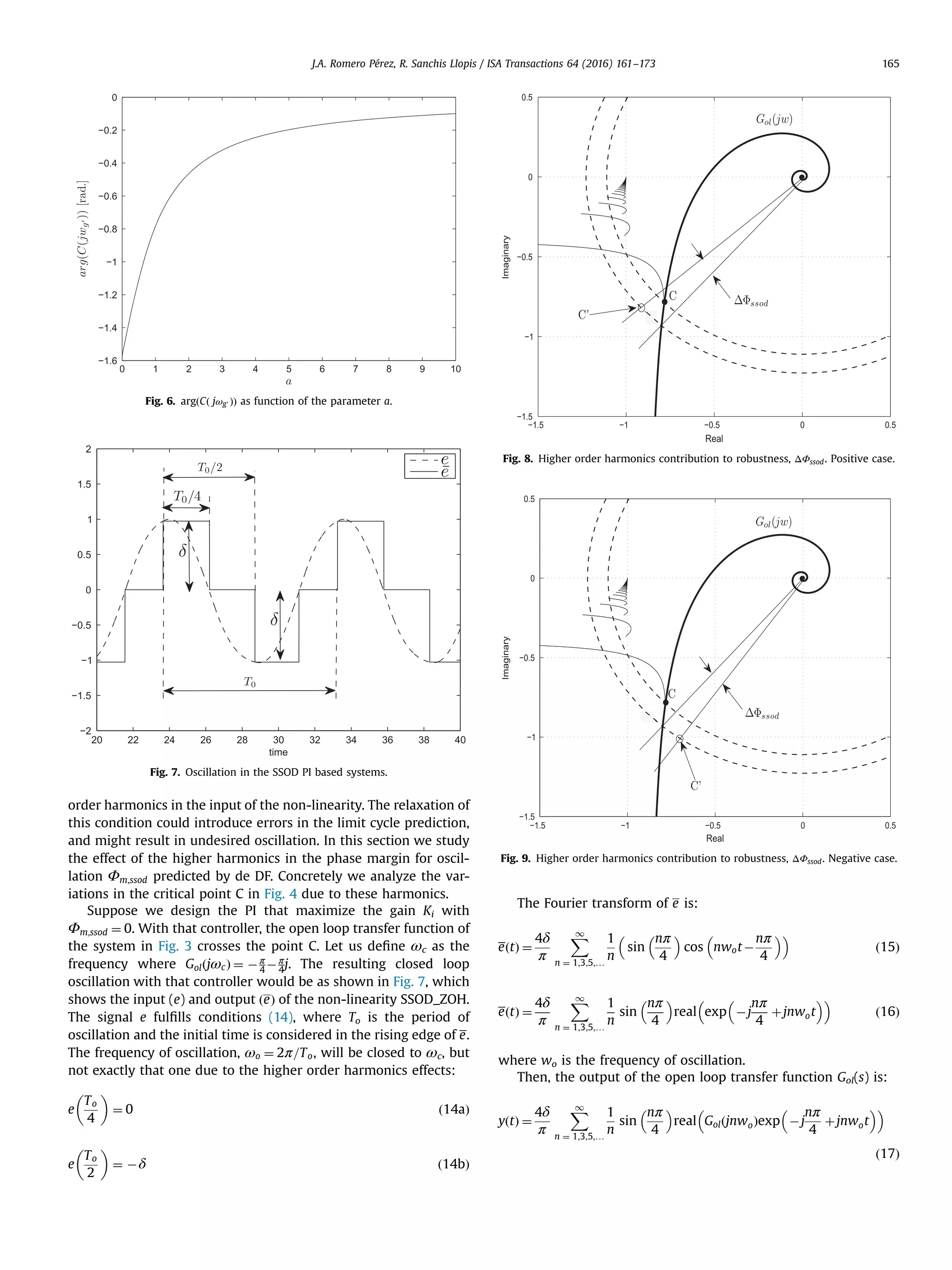
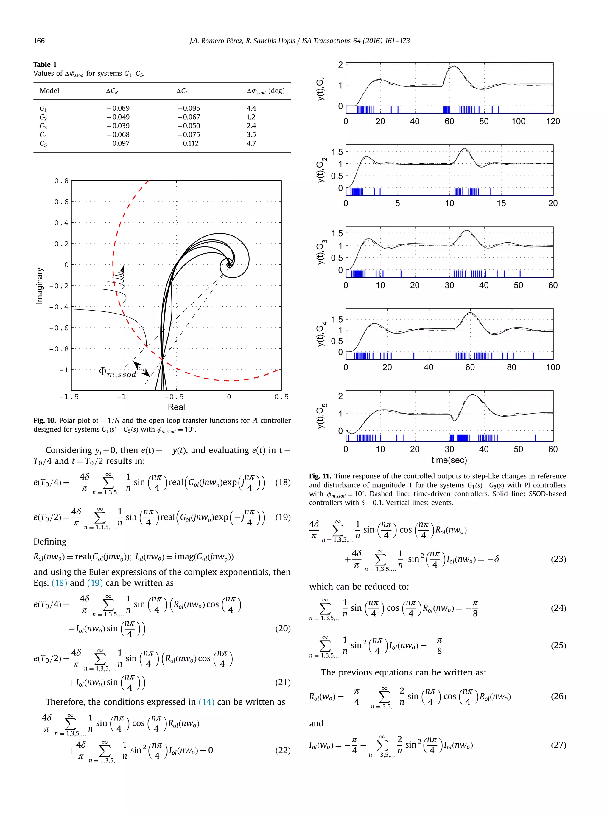
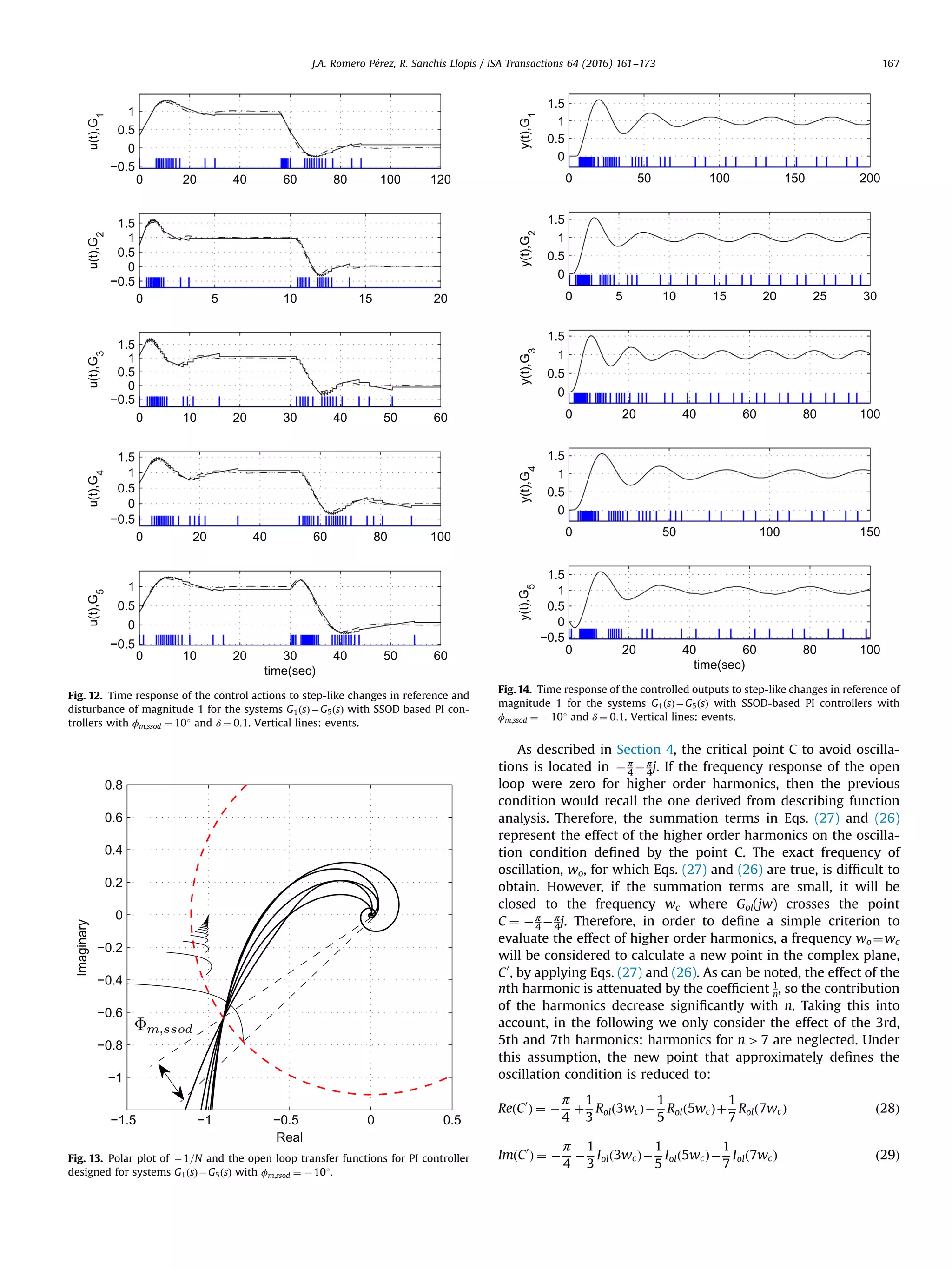
  The limit cyclewill appear if the closed loop transfer function Gol(jw) encircles the new point C0 . Therefore, the distance from that point to the original one, C, is a measure of the validity of the describing function approach. A convenient way to measure that distance, from the robustness point of view is by defining the difference in phase in the following way. Let us define ΔΦssod, as the difference in phase of the open loop transfer function between the point where j GolðjwÞj ¼ jC0 j, and the point C0 , as shown in Figs. 8 and 9. If this difference is negative, it means that the system will oscillate even if it does not cross the C point, i.e. the higher order harmonics decrease the robustness to limit cycles. If this difference is positive, it means that the system will not oscillate even if it crosses the C point, i.e., the higher order harmonics increase the robustness to limit cycles. This fact is illustrated in the next section, where an extensive simulation study is presented. 6. Simulation study In order to verify the applicability of the proposed method, a well known batch of models (30a)–(30e) that summarizes the most common dynamics encountered in industrial processes is used, [19]. G1ðsÞ ¼ eÀ 5s ðsþ1Þ3 ð30aÞ G2ðsÞ ¼ 9 ðsþ1Þðs2 þ2sþ9Þ ð30bÞ G3ðsÞ ¼ 1 ðsþ1Þ4 ð30cÞ G4ðsÞ ¼ 1 ðsþ1Þ7 ð30dÞ G5ðsÞ ¼ 1À2s ðsþ1Þ3 ð30eÞ Table 1 shows the values of ΔΦssod for all the studied models. In all cases ΔΦssod 40, therefore the effect of the higher order harmo- nics is always to increase the robustness to limit cycle respect to the results obtained with the DF technique. The values in columns two and three are the effect of the higher harmonics in the point C, that is: ΔCR ¼ 1 3 Rolð3wcÞÀ1 5 Rolð5wcÞþ1 7 Rolð7wcÞ ð31Þ ΔCI ¼ À1 3 Iolð3wcÞÀ1 5 Iolð5wcÞÀ1 7 Iolð7wcÞ ð32Þ For all these systems SSOD based PI controllers were designed applying the tuning method proposed in the previous section, with ϕm;ssod ¼ 101. Fig. 10 shows the polar plots obtained with the PI controllers. It can be noted that all cases fulfill the robustness conditions ϕm;ssod ¼ 101 and γm Z2, therefore limit cycle oscilla- tions should not appear in the closed loop control systems. This fact is confirmed in Figs. 11 and 12 where the responses for time- driven and SSOD-based controllers are depicted. For the simula- tion of the time-driven controller, fixed sampling periods T ¼ 0:3; 0:05; 0:1; 0:2; 0:2 s have been used for systems G1ðsÞÀG5ðsÞ respectively. For the simulations of the SSOD-based controllers the value of δ ¼ 0:1 has been considered. The instants when events take place with this value of δ are also presented in the figures. As can be noted the responses of conventional and SSOD-based controllers are similar despite the significant reduction of required measurement transmissions in the event based approach. In order to show that the oscillations really appear if the new robustness measure is not ensured, PI controllers have been designed for ϕm;ssod ¼ À101 and γm Z2. In Fig. 13 the polar plots obtained for those PI controllers are shown. All the Nyquist plots intersect the DF plot, predicting the oscillations. Figs. 14 and 15 show the simulations results that confirm the persistent oscillations that appear in the time response. 7. Java based design tool An application has been developed in Java to implement the PI design strategy and to simulate the response of the controlled system to setpoint and disturbance changes. The tool can be downloaded from https://sites.google.com/a/uji.es/freepidtools/ send-on-delta-pi-design-tool. The tool allows to define the desired SOD phase margin and the minimum required gain margin, and to select the value of parameter a with a simple slider, and calculates the controller for that value of a (applying Eqs. (10) and (12)). In addition, the optimum PI controller (solution of optimization problem (13)) can be calculated by simply pressing the button “Maximize Ki”. Furthermore, if “Auto Maximize Ki” is checked, every time the phase margin is changed through the slider, the optimum controller is automatically calculated. The included output response simulator allows changing the value of SOD parameter δ through a slider, making very easy to analyze the effect of δ on the behavior and the number of events. The SSOD-PI scheme is used by default, but the PI-SSOD scheme can also be simulated (with or without dead band). It also allows to simulate the effect of a digital controller implementation with the desired 0 50 100 150 200 0 0.5 1 1.5 u(t),G1 0 5 10 15 20 25 30 0 1 2 u(t),G 2 0 20 40 60 80 100 0 1 2 u(t),G3 0 50 100 150 0 0.5 1 1.5 u(t),G4 0 20 40 60 80 100 0 0.5 1 1.5 u(t),G 5 time(sec) Fig. 15. Time response of the control actions to step-like changes in reference of magnitude 1 for the systems G1ðsÞÀG5ðsÞ with SSOD-based PI controllers with ϕm;ssod ¼ À101 and δ ¼ 0:1. J.A. Romero Pérez, R. Sanchis Llopis / ISA Transactions 64 (2016) 161–173168
• 9.
  sampling period. Fig.16 shows the main window of the application and the time response simulation window. 8. Experimental validation In order to verify the reliability of the proposal, the tuning method was used to design the SSOD based PI for an electro- thermal system. The process to be controlled is composed by a heater resistor attached to an iron plate inside a plastic cover. A switched amplifier drives the resistor, while a thermocouple with an amplifier is used to measure the temperature. The system is completed by a small fan that can be used to apply a disturbance to the plant. A picture of the complete electro-thermal system (without the plastic cover) is presented in Fig. 17. The event based control system in Fig. 1 was implemented using two Modicom-340 PLC with CPU BMX P34 2010 linked through a MODBUS RTU RS485 network with transmission speed of 38,400 bits/s. The implementation scheme is depicted in Fig. 18. The PLC actuating as sensor node has a 4 channel analog input module BMX AMI 0410 where the output of the sensor amplifier is connected. On the other hand, the controller/actuator PLC has an 8 digital input/output module BMX DDM 16022, through which the control action is applied to the actuator amplifier as a PWM signal. Two periodic tasks were defined in both the sensor node and the controller/actuator node respectively. The SENSOR task, which runs with period of 100 ms, sends the values of the error according to the SSOD strategy to the PLC where the CONTROLLER Fig. 16. Java application interface: main window (left) and time response simulation window (right). heater resistor fan actuator amplifier sensor amplifier termo−couple plate Fig. 17. Picture of the electro-thermal process used for the experiment. Fig. 18. Control scheme used for the practical validation of the proposal. J.A. Romero Pérez, R. Sanchis Llopis / ISA Transactions 64 (2016) 161–173 169
• 10.
  task is executed.In the CONTROLLER task a simple Euler dis- cretization of a PI controller with anti windup was implemented running with period of 1 s. The transfer function of the electro-thermal system, Eq. (33), was obtained from the time response of the iron plate temperature to a step like voltage change applied to process input. Two PI controllers were designed using this transfer function according to the method addressed in Section 4.1 for Φm;ssod ¼ À101 and Φm;ssod ¼ 101, both with γm Z8 dB. The controllers were designed with the Java application described in Section 7. Figs. 19 and 20 show the resulting design for Φm;ssod ¼ À101 and Φm;ssod ¼ þ101 respectively. The most important characteristics of the designs are summarized in Table 2: GðsÞ ¼ 2:66 ð1þ26:5sÞ2 ð1þ244sÞ ð33Þ According to the values of Φm and γm, stable closed loop responses should be obtained for both controllers when imple- mented in a time-driven approach with a properly selected sample time. However, if SSOD sampling strategy is used, the controller designed with Φm;ssod ¼ À101 will induce limit cycle oscillations, as predicted in this paper. This fact is confirmed by the actual system response which is shown in Fig. 21, where the response to a step change in the setpoint (at t¼460 s) and to a step change in the disturbance (at t¼1700 s) are shown. It can be noted that for time greater than 3000 s, after the disturbance correction, the system response presents limit cycle oscillations, which can be seen in more detail in Fig. 22. On the other hand, the controller designed with Φm;ssod ¼ 101 produces a stable response without limit cycles, as is shown in Fig. 23. It is worth highlighting that in the actual application, as well as in simulations presented in Section 6, the close loop response of the SSOD based system is similar to that of the time- driven case, which has been obtained here by continuous simu- lation using the model (33) and is presented in Fig. 24. 9. Conclusions In this paper we have analyzed the conditions that produce oscillations in event based PI controllers, assuming a symmetric send on delta scheme. The problem is addressed by means of the describing function (DF). A critical point has been found in the DF plot that determines the existence of oscillations. Conditions for oscillation are reduced to the encirclement of that point by the Nyquist plot. Taking this into account, a new method for tuning SSOD based PI controller is presented to avoid the limit cycles, including the introduction of a new robustness to oscillations performance measure. The effect of higher order harmonics in the tuning method has also been studied. Surprisingly, it has been found that, for most systems, the contribution of higher order harmonics does not impose further restrictions to the tuning method. Instead, it pro- vides an additional margin to avoid oscillations, that increases the one imposed by the DF method. Another interesting conclusion is that the appearance of limit cycles does not depend on the value of δ, even if the higher order harmonics are considered. The value of δ affects the amplitude of oscillations (if they appear), the steady state error and the number of events (measurements transmission). Fig. 19. Java application interface: results for the design with Φssos ¼ À101. J.A. Romero Pérez, R. Sanchis Llopis / ISA Transactions 64 (2016) 161–173170
• 11.
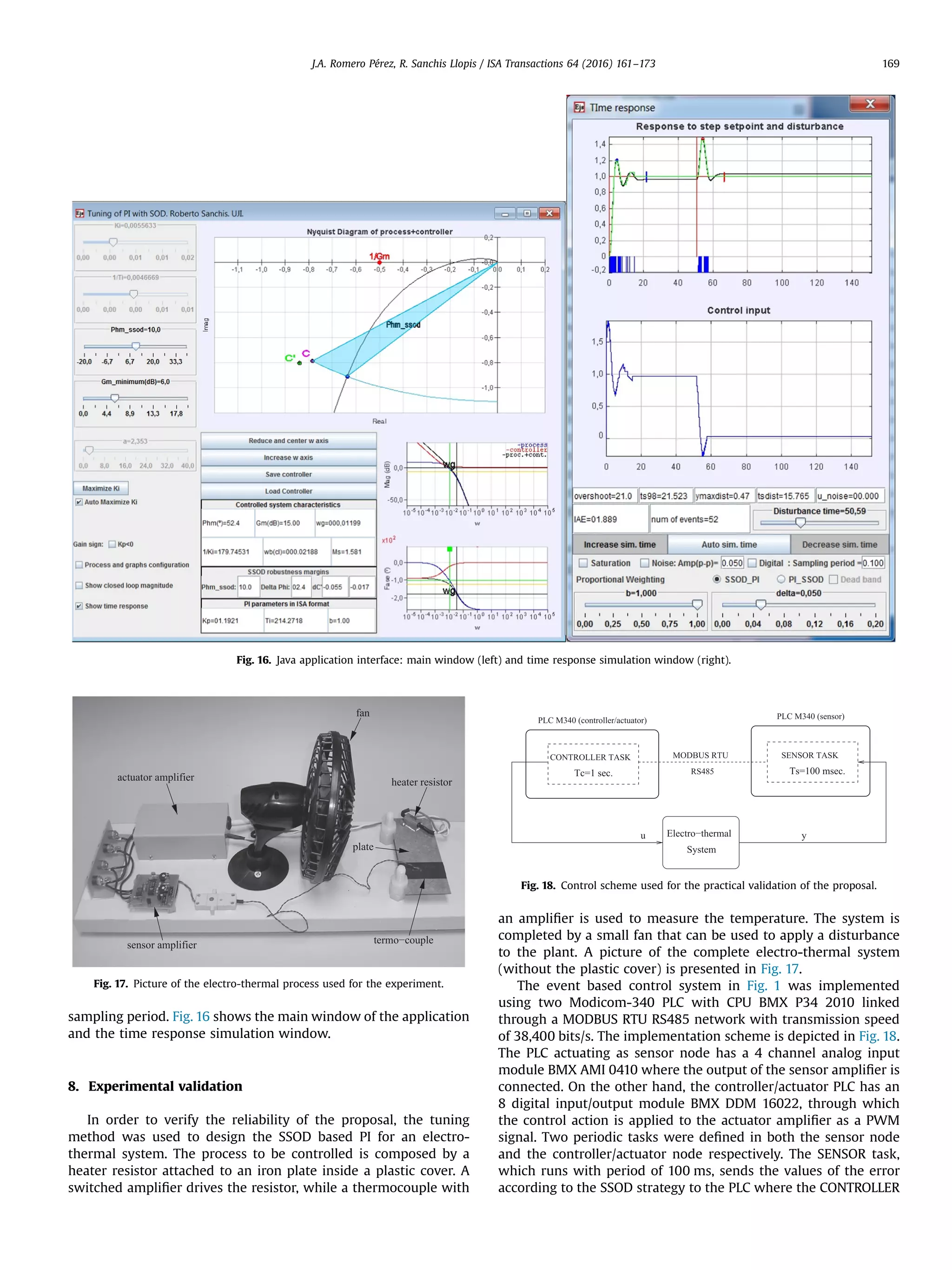
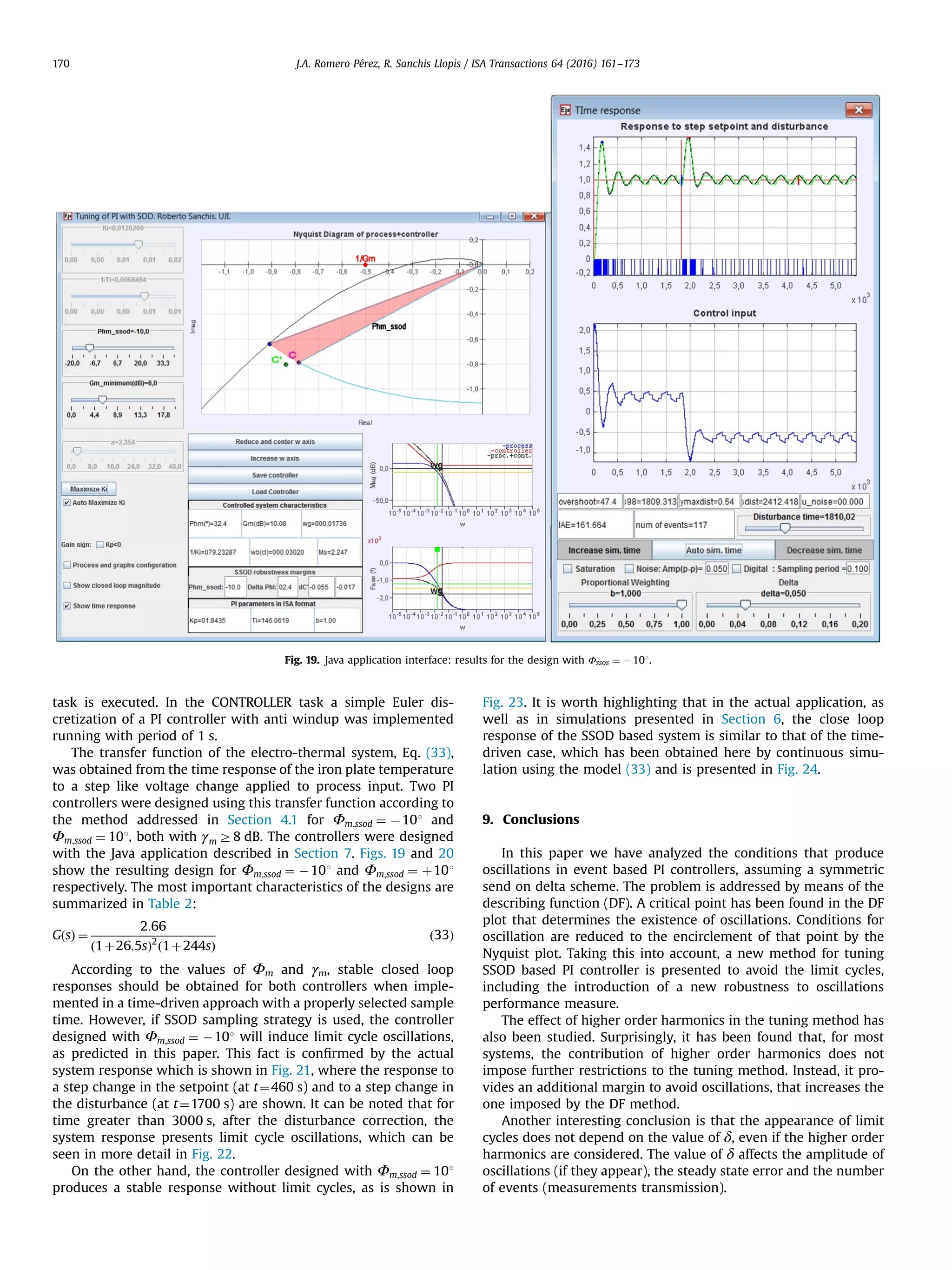
  The proposed ideasare illustrated in simulations with a batch of models widely used in the literature to test PI design methods. The feasibility of the proposal has been also corroborated by the application to the control of an actual laboratory scale electro- thermal system. Additionally, the tuning method has been implemented in an easy to use Java based application (https:// sites.google.com/a/uji.es/freepidtools/send-on-delta-pi-design- Fig. 20. Java application interface: results for the design with Φssos ¼ þ101. Table 2 PI design results for the electro-thermal system. Φm;ssod ΔΦssod γmðdBÞ Kp Ti (s) À10° 2.4° 10 1.84 146.06 10° 2.4° 15 1.19 214.21 0 500 1000 1500 2000 2500 3000 3500 45 50 55 60 65 time [sec.] y[ o C] 0 500 1000 1500 2000 2500 3000 3500 0 10 20 30 time [sec.] u[V] Fig. 21. Time response of the controlled outputs to step-like changes in reference and disturbance for the electro-thermal system with PI controllers with ϕm;ssod ¼ À101 and δ ¼ 0:5 1C. 0 500 1000 1500 2000 2500 3000 3500 4000 49 49.5 50 50.5 51 time [sec.] y[o C] 0 500 1000 1500 2000 2500 3000 3500 4000 5 6 7 8 time [sec.] u[V] Fig. 22. Temperature oscillations in the electro-thermal system with PI controllers with ϕm;ssod ¼ À101 and δ ¼ 0:5 1C. J.A. Romero Pérez, R. Sanchis Llopis / ISA Transactions 64 (2016) 161–173 171
• 12.
  tool), which wasdeveloped to aid the design and simulation of SSOD based PI controllers. Acknowledgements This work has been supported by the MICINN under grant DPI2011-27845-C02–02. Appendix A. Describing function of the SSOD_ZOH sampler The output equation of SSOD_ZOH sampler, whose input/out- put relation is presented in Fig. 2, is: eðtÞ ¼ ðiþ1Þδ if eðtÞZðiþ1Þδ and eðtÀ Þ ¼ iδ; iAZ ðiÀ1Þδ if eðtÞrðiÀ1Þδ and eðtÀ Þ ¼ iδ iδ if eðtÞA½ðiÀ1Þδ; ðiþ1ÞδŠ and eðtÀ Þ ¼ iδ 8 : ðA:1Þ For a sinusoidal input eðϕÞ ¼ A sin ðϕÞ, the output of the SSOD_ZOH block can be expressed as eðϕÞ ¼ δ Xi k ¼ 1 sgn deðϕÞ dϕ ϕk ! 8ϕ; ϕi oϕoϕi þ1 ¼ δ Xi k ¼ 1 sgn cos ϕk À Á 8ϕ; ϕi oϕoϕi þ1 ðA:2Þ where sgnðeÞ ¼ 1 if e40 À1 if eo0 0 if e ¼ 0 8 : ðA:3Þ The SSOD_ZOH sampler is an odd no-linearity where the his- tory of the input determines the value of the output in the multiple-valued regions. The describing function for this kind of nonlinearity can be calculated as: NðAÞ ¼ 2j πA Z π 0 eðϕÞexpðÀjϕÞdϕ ¼ 2j πA Z ϕ2 ϕ1 sgnð cos ϕ1ÞδexpðÀjϕÞdϕ þ Z ϕ3 ϕ2 ðsgnð cos ϕ1Þþsgnð cos ϕ2ÞÞδexpðÀjϕÞdϕ þ⋯⋯þ Z ϕi þ 1 ϕi Xi k ¼ 1 ðsgnð cos ϕkÞÞδexpðÀjϕÞdϕ þ⋯⋯þ Z π ϕn Xn k ¼ 1 ðsgnð cos ϕkÞÞδexpðÀjϕÞdϕ ! Applying the addition of integration on intervals, the previous equation can be rewritten as NðAÞ ¼ 2Dj πA Z π ϕ1 sgnð cos ϕ1ÞexpðÀjϕÞdϕ þ Z π ϕ2 sgnð cos ϕ2ÞexpðÀjϕÞdϕ þ⋯⋯þ Z π ϕi sgnð cos ϕiÞexpðÀjϕÞdϕ þ⋯⋯þ Z π ϕn sgnð cos ϕnÞexpðÀjϕÞdϕ ! ¼ 2Dj πA Xn k ¼ 1 sgnð cos ϕkÞ Z π ϕk expðÀjϕÞdϕ ! ðA:4Þ Taking into account that Z π ϕk expðÀjϕÞdϕ ¼ Àjð1þexpðÀjϕkÞÞ and expðÀjϕkÞ ¼ cos ϕk Àj sin ϕk Eq. (A.4) results in NðAÞ ¼ 2δ πA Xn k ¼ 1 sgnð cos ϕkÞð1þ cos ϕkÞþj Xn k ¼ 1 sgnð cos ϕkÞ sin ϕk ! ðA:5Þ Since for m ¼ A δ # ) ϕm rπ=2oϕmþ 1 the following identity is fulfilled cos ϕmÀk ¼ À cos ϕmþk; k ¼ 1⋯mÀ1; ðA:6Þ 0 500 1000 1500 2000 2500 3000 3500 45 50 55 60 65 time [sec.] y[ o C] 0 500 1000 1500 2000 2500 3000 3500 5 10 15 20 time [sec.] u[V] Fig. 23. Time response of the controlled outputs to step-like changes in reference and disturbance for the electro-thermal system with PI controllers with ϕm;ssod ¼ 101 and δ ¼ 0:5 1C. 0 500 1000 1500 2000 2500 3000 3500 0 5 10 15 time(sec) Δu[V] 0 500 1000 1500 2000 2500 3000 3500 0 5 10 15 time(sec) Δy[ o C] Fig. 24. Time response of the controlled output and the control action to step-like changes in reference and disturbance obtained by continuous simulation con- sidering the model (33) and the PI controllers designed with ϕm;ssod ¼ 101. J.A. Romero Pérez, R. Sanchis Llopis / ISA Transactions 64 (2016) 161–173172
• 13.
  the terms inthe right hand side of Eq. (A.5) are transformed to Xn k ¼ 1 sgnð cos ϕkÞð1þ cos ϕkÞ ¼ 1þ cos ϕm þ2 Xm À1 k ¼ 1 cos ϕk ðA:7Þ and Xn k ¼ 1 sgnð cos ϕkÞ sin ϕk ¼ sin ϕm ðA:8Þ Therefore, Eq. (A.5) can be rewritten as follows NðAÞ ¼ 2δ πA 1þ cos ϕm þ2 XmÀ 1 k ¼ 1 cos ϕk Àj sin ϕm ! ðA:9Þ The previous expression for N(A) only depends on ϕk rπ=2, so the following identities can be used to write de describing func- tion in terms of the SSOD_ZOH nonlinearity parameter δ: sin ϕk ¼ k δ A ) ϕk ¼ arcsin k δ A ðA:10Þ cos ϕk ¼ ffiffiffiffiffiffiffiffiffiffiffiffiffiffiffiffiffiffiffiffiffiffiffi 1À k δ A 2 s ðA:11Þ Using Eqs. (A.10) and (A.11) the describing function N(A) can be rewritten as follows: NðA; δÞ ¼ 2δ πA 1þ ffiffiffiffiffiffiffiffiffiffiffiffiffiffiffiffiffiffiffiffiffiffiffiffiffi 1À m δ A 2 s þ2 XmÀ 1 k ¼ 1 ffiffiffiffiffiffiffiffiffiffiffiffiffiffiffiffiffiffiffiffiffiffiffi 1À k δ A 2 s2 4 3 5Àjm 2δ2 πA2 ðA:12Þ References [1] Feeney L, Nilsson M. Investigating the energy consumption of a wireless network interface in an ad hoc networking environment. In: Proceedings of twentieth annual joint conference of the IEEE computer and communications societies, INFOCOM 2001, vol. 3. IEEE, Anchorage, Alaska, United States; 2001. p. 1548–57. http://dx.doi.org/10.1109/INFCOM.2001.916651. [2] Miskowicz M. Send-on-delta concept: an event-based data reporting strategy. Sensors 2006;6(1):49–63. [3] Dormido S, Sanchez J, Kofman E. Muestreo, control y comunicacion basados en eventos. Rev Iberoam Autom Inform Ind RIAI 2008;5(1):5–26. [4] Ploennigs J, Vasyutynskyy V, Kabitzsch K. Comparative study of energy- efficient sampling approaches for wireless control networks. IEEE Trans Ind Inform 2010;6(3):416–24. http://dx.doi.org/10.1109/TII.2010.2051812. [5] Årzén K-E. A simple event-based PID controller. In: Proceedings of 14th world congress of IFAC, vol. 18. Beijing; 1999. p. 423–8. [6] Durand S, Marchand N. An event-based PID controller with low computational cost. In: Fesquet L, Torrésani B, editors. 8th international conference on sam- pling theory and applications (SampTA'09); 2009. 〈http://hal.archives- ouvertes.fr/hal-00393031〉. [7] Durand S, Marchand N. Further results on event-based PID controller. In: Proceedings of the European control conference 2009. Budapest, Hongrie; 2009. p. 1979–84. 〈http://hal.archives-ouvertes.fr/hal-00368535〉. [8] Vasyutynskyy V, Kabitzsch K. A comparative study of PID control algorithms adapted to send-on-delta sampling. In: 2010 IEEE international symposium on industrial electronics (ISIE); 2010. p. 3373–9. http://dx.doi.org/10.1109/ISIE. 2010.5637997. [9] Vasyutynskyy V, Kabitzsch K. Time constraints in PID controls with send-on- delta. In: Juanole G, Hong SH, editors. Fieldbuses and networks in industrial and embedded systems, vol. 8; 2009. [10] Beschi M, Dormido S, Sanchez J, Visioli A. Characterization of symmetric send- on-delta PI controllers. J Process Control 2012;22(10):1930–45. http://dx.doi. org/10.1016/j.jprocont.2012.09.005 http://linkinghub.elsevier.com/retrieve/pii/ S0959152412002247. [11] Chacón J, Sánchez J, Visioli A, Yebra L, Dormido S. Characterization of limit cycles for self-regulating and integral processes with PI control and send-on- delta sampling. J Process Control 2013;23(6):826–38. http://dx.doi.org/ 10.1016/j.jprocont.2013.04.001. [12] Beschi M, Visioli A. Tuning of symmetric send-on-delta proportional-integral controllers. IET Control Theory Appl 2014;8(4):248–59. http://dx.doi.org/10. 1049/iet-cta.2013.0048. [13] Beschi M, Dormido S, Sánchez J, Visioli A. Closed-loop automatic tuning technique for an event-based PI controller. Ind Eng Chem Res 2015; 54(24):6362–70. http://dx.doi.org/10.1021/acs.iecr.5b01024. [14] Beschi M, Dormido S, Sanchez J, Visioli A. Stability analysis of symmetric send- on-delta event-based control systems. In: 2013 American control conference (ACC); 2013. p. 1771–6. http://dx.doi.org/10.1109/ACC.2013.6580092. [15] Leva A, Terraneo F. Low power synchronisation in wireless sensor networks via simple feedback controllers: the flopsync scheme. In: 2013 American control conference (ACC); 2013. p. 5017–22. [16] Gelb A, VanderVelde WE. Multiple-input describing functions and nonlinear system design. New York, NY, USA: McGraw-Hill; 1968. [17] Romero J, Sanchis R, Peñarrocha I. A simple rule for tuning event-based pid controllers with symmetric send-on-delta sampling strategy. In: 2014 IEEE 19th conference on emerging technologies factory automation (ETFA); 2014. [18] Sanchis R, Romero JA, Balaguer P. Tuning of pid controllers based on simplified single parameter optimisation. Int J Control 2010;83(9):1785–98. http://dx.doi. org/10.1080/00207179.2010.495162. [19] Panagopoulos H, Astrom KJ, Hagglund T. Design of PID controllers based on constrained optimization. IEE Proc – Control Theory Appl 2002;149(1):32–40. J.A. Romero Pérez, R. Sanchis Llopis / ISA Transactions 64 (2016) 161–173 173