This document provides an overview of image analysis and pattern recognition techniques for remote sensing applications using algorithms in ENVI/IDL. It covers topics such as image statistics, transformations like Fourier transforms and principal components analysis, radiometric enhancement, topographic modeling, image registration, sharpening, change detection, classification (both unsupervised and supervised), and hyperspectral analysis. The intended audience is researchers and practitioners working with remote sensing images.


![1.1. MULTISPECTRAL SATELLITE IMAGES 3 or digital number g and at-sensor radiance f is determined by the sensor calibration as measured (and maintained) by the satellite image provider: f = Cg(i, j) + fmin where C = (fmax − fmin)/255, in which fmax and fmin are maximum and minimum mea- surable radiances at the sensor. Atmospheric scattering and absorption models are used to calculate surface reflectance from the observed at-sensor radiance, as it is the reflectance which is directly related to the physical properties of the surface being examined. Various conventions can be used for storing the image array g(i, j) in computer memory or on storage media. In band interleaved by pixel (BIP) format, for example, a two-channel, 3 × 3 pixel image would be stored as g1(1, 1) g2(1, 1) g1(2, 1) g2(2, 1) g1(3, 1) g2(3, 1) g1(1, 2) g2(1, 2) g1(2, 2) g2(2, 2) g1(3, 2) g2(3, 2) g1(1, 3) g2(1, 3) g1(2, 3) g2(2, 3) g1(3, 3) g2(3, 3), whereas in band interleaved by line (BIL) it would be stored as g1(1, 1) g1(2, 1) g1(3, 1) g2(1, 1) g2(2, 1) g2(3, 1) g1(1, 2) g1(2, 2) g1(3, 2) g2(2, 1) g1(2, 2) g2(2, 3) g1(1, 3) g2(2, 3) g1(3, 3) g2(3, 1) g1(2, 3) g2(3, 3), and in band sequential (BSQ) format it is stored as g1(1, 1) g1(2, 1) g1(3, 1) g1(1, 2) g1(2, 2) g1(3, 2) g1(1, 3) g1(2, 3) g1(3, 3) g2(1, 1) g2(2, 1) g2(3, 1) g2(1, 2) g2(2, 2) g2(3, 2) g2(1, 3) g2(2, 3) g2(3, 3). In the computer language IDL, so-called row major indexing is used for arrays and the elements in an array are numbered from zero. This means that, if a gray-scale image g is stored in an IDL array variable G, then the intensity value g(i, j) is addressed as G[i-1,j-1]. An N-band multispectral image is stored in BIP format as an N × c × r array in IDL, in BIL format as a c × N × r and in BSQ format as an c × r × N array. Auxiliary information, such as image acquisition parameters and georeferencing, is nor- mally included with the image data on the same file, and the format may or may not make use of compression algorithms. Examples are the geoTIFF1 file format used for example by Space Imaging Inc. for distributing Carterra(c) imagery and which includes lossless compres- sion, the HDF (Hierachical Data Format) in which for example ASTER images are distributed and the cross-platform PCDSK format employed by PCI Geomatics with its image process- ing software, which is in plain ASCII code and not compressed. ENVI uses a simple “flat binary” file structure with an additional ASCII header file. 1geoTIFF refers to TIFF files which have geographic (or cartographic) data embedded as tags within the TIFF file. The geographic data can then be used to position the image in the correct location and geometry on the screen of a geographic information display.](https://image.slidesharecdn.com/mortonjohncanty-imageanalysisandpatternrecognitionforremotesensingwithalgorithmsinenvi-idl-190425063306/75/Morton-john-canty-image-analysis-and-pattern-recognition-for-remote-sensing-with-algorithms-in-envi-idl-11-2048.jpg)
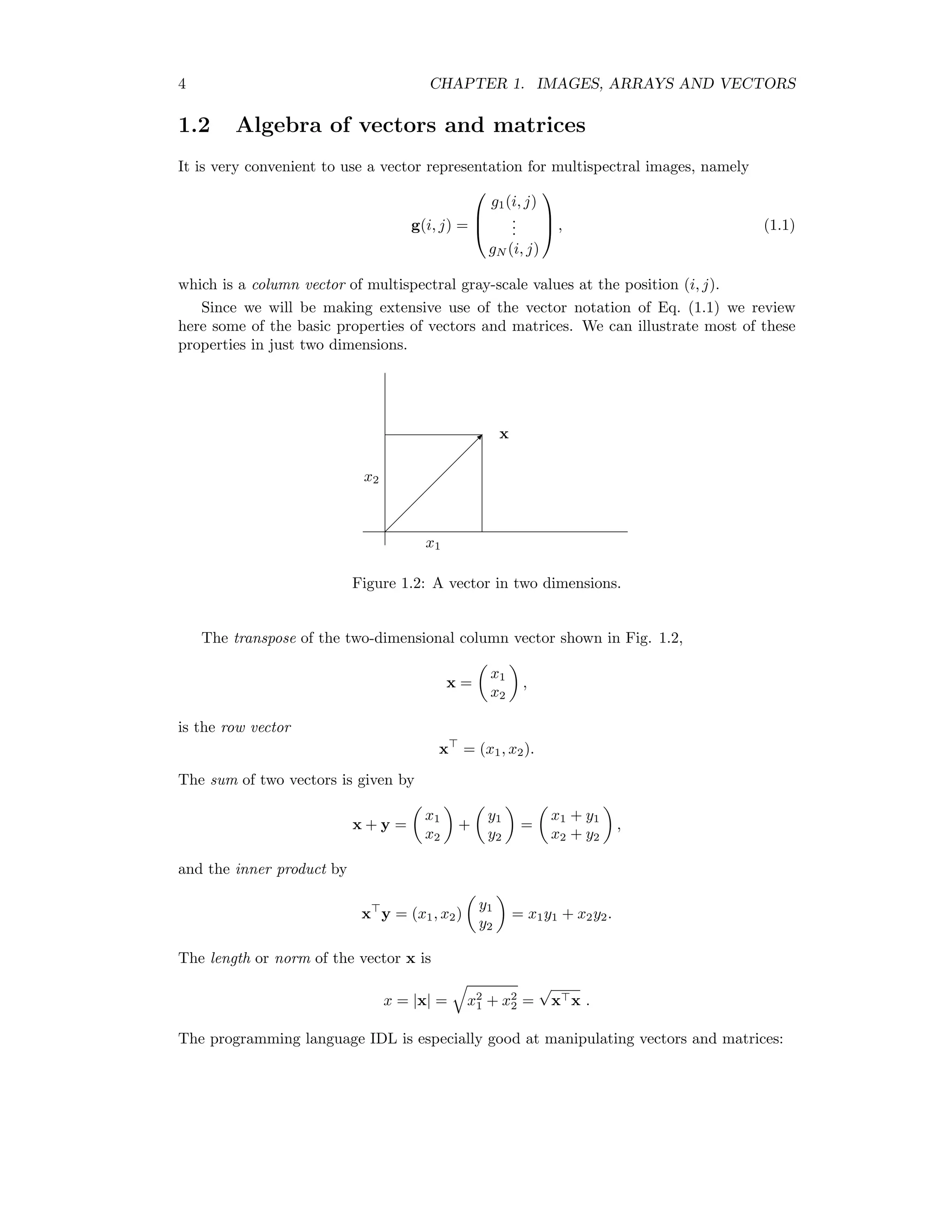
![1.2. ALGEBRA OF VECTORS AND MATRICES 5 IDL x=[[1],[2]] IDL print,x 1 2 IDL print,transpose(x) 1 2 b X x yθ x cos θ Figure 1.3: The inner product. The inner product can be written in terms of the vector lengths and the angle θ between the two vectors as x y = |x||y| cos θ = xy cos θ, see Fig. 1.3. If θ = 90o the vectors are orthogonal so that x y = 0. Any vector can be decomposed into orthogonal unit vectors: x = x1 x2 = x1 1 0 + x2 0 1 . A two-by-two matrix is written A = a11 a12 a21 a22 . When a matrix is multiplied with a vector the result is another vector, e.g. Ax = a11 a12 a21 a22 x1 x2 = a11x1 + a12x2 a21x1 + a22x2 . The IDL operator for matrix and vector multiplication is ##. IDL a=[[1,2],[3,4]] IDL print,a 1 2 3 4 IDL print,a##x 5 11](https://image.slidesharecdn.com/mortonjohncanty-imageanalysisandpatternrecognitionforremotesensingwithalgorithmsinenvi-idl-190425063306/75/Morton-john-canty-image-analysis-and-pattern-recognition-for-remote-sensing-with-algorithms-in-envi-idl-13-2048.jpg)
![1.3. EIGENVALUES AND EIGENVECTORS 7 matrices. As we will see later, covariance matrices are always symmetric. A matrix A is symmetric if it doesn’t change when it is transposed, i.e. if A = A . Very often we have to solve the so-called eigenvalue problem, which is to find eigenvectors x and eigenvalues λ that satisfy the equation Ax = λx or, equivalently, a11 a12 a21 a22 x1 x2 = λ x1 x2 . This is the same as the two equations (a11 − λ)x1 + a12x2 = 0 a21x1 + (a22 − λ)x2 = 0. (1.2) If we eliminate x1 and make use of the symmetry a12 = a21, we obtain [(a11 − λ)(a22 − λ) − a2 12]x2 = 0. In general x2 = 0, so we must have (a11 − λ)(a22 − λ) − a2 12 = 0, which is known as the characteristic equation for the eigenvalue problem. It is a quadratic equation in λ with solutions λ(1) = 1 2 a11 + a22 + (a11 + a22)2 − 4(a11a22 − a2 12) λ(2) = 1 2 a11 + a22 − (a11 + a22)2 − 4(a11a22 − a2 12) . (1.3) Thus there are two eigenvalues and, correspondingly, two eigenvectors x(1) and x(2) , which can be obtained by substituting λ(1) and λ(2) into (1.2) and solving for x1 and x2. It is easy to show that the eigenvalues are orthogonal (x(1) ) x(2) = 0. The matrix formed by the two eigenvectors, u = (x(1) , x(2) ) = x (1) 1 x (2) 1 x (1) 2 x (2) 2 , is said to diagonalize the matrix a. That is u Au = λ(1) 0 0 λ(2) . (1.4) We can illustrate the whole procedure in IDL as follows:](https://image.slidesharecdn.com/mortonjohncanty-imageanalysisandpatternrecognitionforremotesensingwithalgorithmsinenvi-idl-190425063306/75/Morton-john-canty-image-analysis-and-pattern-recognition-for-remote-sensing-with-algorithms-in-envi-idl-15-2048.jpg)
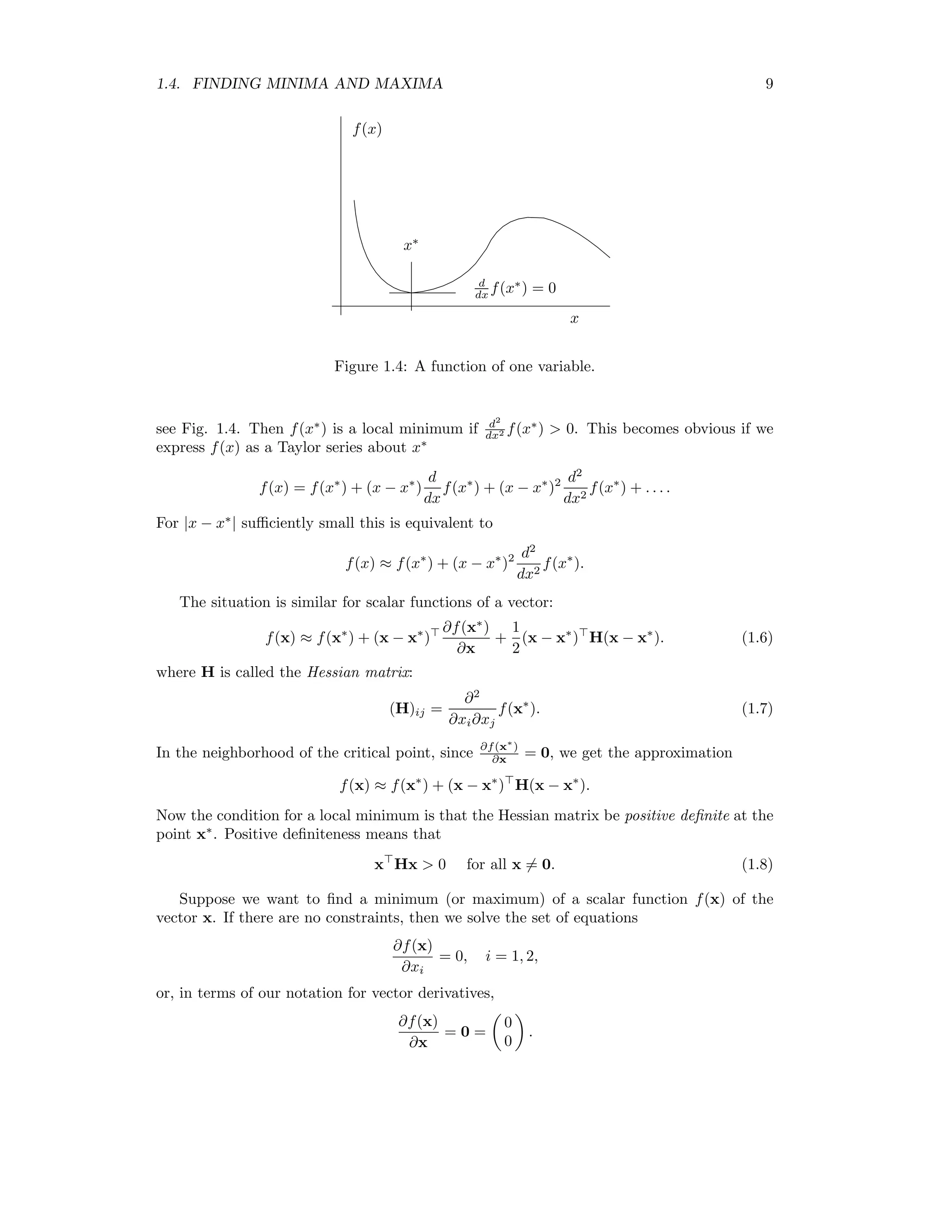
![8 CHAPTER 1. IMAGES, ARRAYS AND VECTORS IDL a=float([[1,2],[2,3]]) IDL print,a 1.00000 2.00000 2.00000 3.00000 IDL print,eigenql(a,eigenvectors=u,/double) 4.2360680 -0.23606798 IDL print,transpose(u)##a##u 4.2360680 -2.2204460e-016 -1.6653345e-016 -0.23606798 Note that, after diagonalization, the off-diagonal elements are not precisely zero due to rounding errors in the computation. All of the above properties generalize easily to N dimensions. 1.4 Finding minima and maxima In order to maximize some desirable property of a multispectral image, such as signal to noise or spread in intensity, we often need to take derivatives of vectors. A vector (partial) derivative in two dimensions is written ∂ ∂x and is defined as the vector ∂ ∂x = 1 0 ∂ ∂x1 + 0 1 ∂ ∂x2 . Many of the operations with vector derivatives correspond exactly to operations with or- dinary scalar derivatives (They can all be verified easily by writing out the expressions component-by component): ∂ ∂x (x y) = y analogous to ∂ ∂x xy = y ∂ ∂x (x x) = 2x analogous to ∂ ∂x x2 = 2x The scalar expression x Ay, where A is a matrix, is called a quadratic form. We have ∂ ∂x (x Ay) = Ay ∂ ∂y (x Ay) = A x and ∂ ∂x (x Ax) = Ax + A x. Note that, if A is a symmetrix matrix, this last equation can be written ∂ ∂x (x Ax) = 2Ax. Suppose x∗ is a critical point of the function f(x), i.e. d dx f(x∗ ) = d d f(x) x=x∗ = 0, (1.5)](https://image.slidesharecdn.com/mortonjohncanty-imageanalysisandpatternrecognitionforremotesensingwithalgorithmsinenvi-idl-190425063306/75/Morton-john-canty-image-analysis-and-pattern-recognition-for-remote-sensing-with-algorithms-in-envi-idl-16-2048.jpg)
![10 CHAPTER 1. IMAGES, ARRAYS AND VECTORS However suppose that x is constrained by the equation g(x) = 0. For example, we might have g(x) = x2 1 + x2 2 − 1 = 0 which constrains x to lie on a circle of radius 1. Finding an minimum of f subject to g = 0 is equivalent to finding an unconstrained minimum of f(x) + λg(x), (1.9) where λ is called a Lagrange multiplier and is treated like an additional variable, see [Mil99]. That is, we solve the set of equations ∂ ∂xi (f(x) + λg(x)) = 0, i = 1, 2 ∂ ∂λ (f(x) + λg(x)) = 0. (1.10) The latter equation is just g(x) = 0. For example, let f(x) = ax2 1 + bx2 2 and g(x) = x1 + x2 − 1. Then we get the three equations ∂ ∂x1 (f(x) + λg(x)) = 2ax1 + λ = 0 ∂ ∂x2 (f(x) + λg(x)) = 2bx2 + λ = 0 ∂ ∂λ (f(x) + λg(x)) = x1 + x2 − 1 = 0 The solution is x1 = b a + b , x2 = a a + b .](https://image.slidesharecdn.com/mortonjohncanty-imageanalysisandpatternrecognitionforremotesensingwithalgorithmsinenvi-idl-190425063306/75/Morton-john-canty-image-analysis-and-pattern-recognition-for-remote-sensing-with-algorithms-in-envi-idl-18-2048.jpg)


![14 CHAPTER 2. IMAGE STATISTICS For continuous random variables, such as the measured radiance at a satellite sensor, the distribution function is not expressed in terms of discrete probabilities, but rather in terms of a probability density function p(x), where p(x)dx is the probability that the value of the random variable X lies in the interval [x, x + dx]. Then P(x) = Pr(X ≤ x) = x −∞ p(t)dt and, of course, P(−∞) = 0, P(∞) = 1. Two random variables X and Y are said to be independent when Pr(X ≤ x and Y ≤ y) = Pr(X ≤ x, Y ≤ y) = P(x)P(y). The mean or expected value of a random variable X is written X and is defined in terms of the probability density function: X = ∞ −∞ xp(x)dx. The variance of X, written var(X) is defined as the expected value of the random variable (X − X )2 , i.e. var(X) = (X − X )2 . In terms of the probability density function, it is given by var(X) = ∞ −∞ (x − X )2 p(x)dx. Two simple but very useful identities follow from the definition of variance: var(X) = X2 − X 2 var(aX) = a2 var(X). (2.1) 2.2 The normal distribution It is often the case that random variables are well-described by the normal or Gaussian probability density function p(x) = 1 √ 2πσ exp(− 1 2σ2 (x − µ)2 ). In that case X = µ, var(X) = σ2 . The expected value of pixel intensities G(x) = G1(x) G2(x) ... GN (x) ,](https://image.slidesharecdn.com/mortonjohncanty-imageanalysisandpatternrecognitionforremotesensingwithalgorithmsinenvi-idl-190425063306/75/Morton-john-canty-image-analysis-and-pattern-recognition-for-remote-sensing-with-algorithms-in-envi-idl-22-2048.jpg)
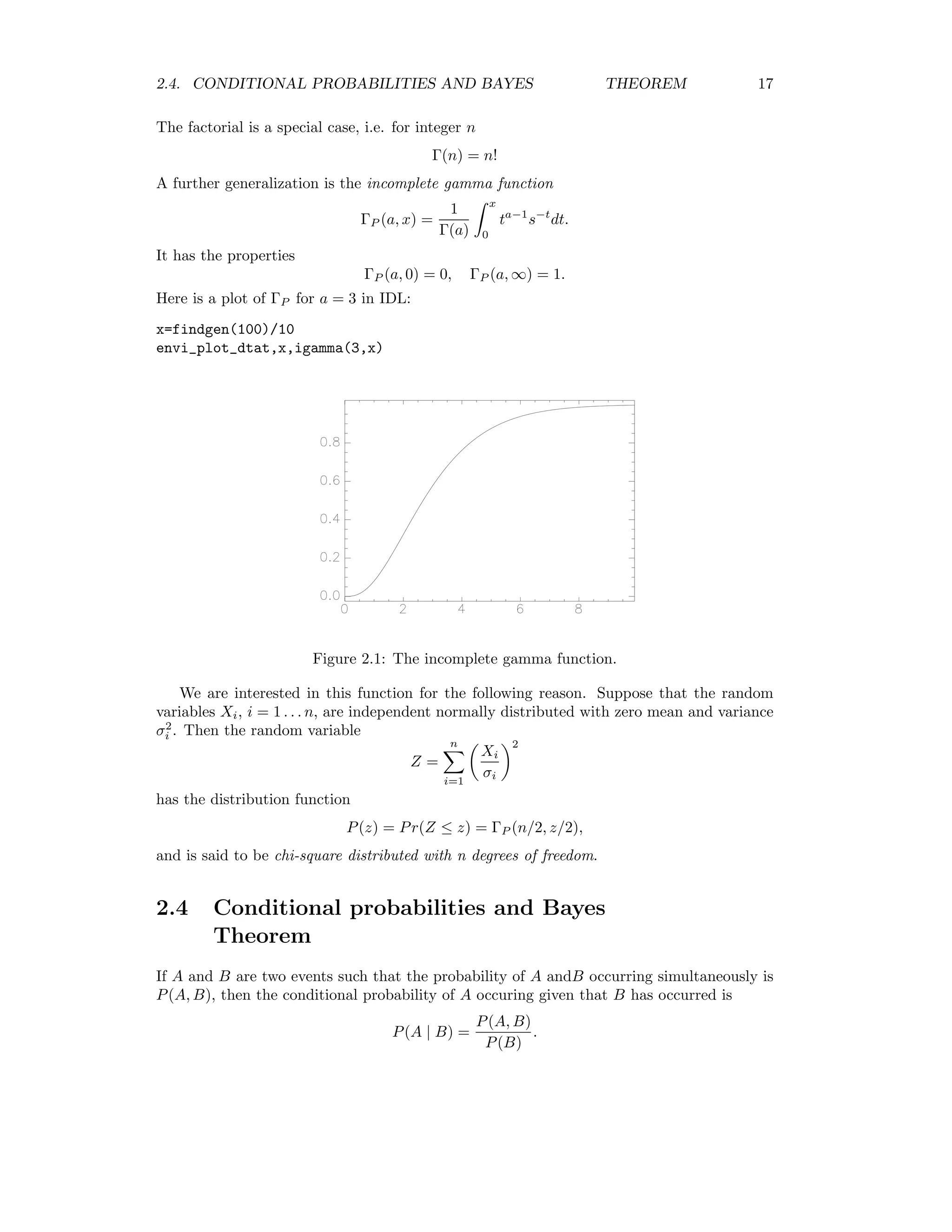
![16 CHAPTER 2. IMAGE STATISTICS This is obvious in two dimensions, since we have var(a G) = cov(a1G1 + a2G2, a1G1 + a2G2) = a2 1var(G1) + a1a2cov(G1, G2) + a1a2cov(G2, G1) + a2 2var(G2) = (a1, a2) var(G1) cov(G1, G2) cov(G2, G1) var(G2) a1 a2 . Variance is always nonnegative and the vector a in (2.2) is arbitrary, so we have a Σa ≥ 0 for all a. The covariance matrix is therefore said to be positive semi-definite. The correlation matrix C is similar to the covariance matrix, except that each matrix element (i, j) is normalized to var(Gi)var(Gj). In two dimensions C = 1 ρ12 ρ21 1 = 1 cov(G1,G2) √ var(G1)var(G2) cov(G2,G1) √ var(G1)var(G2) 1 = 1 σ12 σ1σ2 σ21 σ1σ2 1 . The following ENVI/IDL program calculates and prints out the covariance matrix of a multispectral image: envi_select, title=’Choose multispectral image’,fid=fid,dims=dims,pos=pos if (fid eq -1) then return num_cols = dims[2]-dims[1]+1 num_rows = dims[4]-dims[3]+1 num_pixels = (num_cols*num_rows) num_bands = n_elements(pos) samples=intarr(num_bands,n_elements(num_pixels)) for i=0,num_bands-1 do samples[i,*]=envi_get_data(fid=fid,dims=dims,pos=pos[i]) print, correlate(samples,/covariance,/double) end ENVI .GO 111.46663 82.123236 159.58377 133.80637 82.123236 64.532431 124.84815 104.45298 159.58377 124.84815 246.18004 205.63420 133.80637 104.45298 205.63420 192.70367 2.3 A special function If n is an integer, the factorial of n is defined by n! = n(n − 1) · · · 1, 1! = 0! = 1. The generalization of this to non-integers z is the gamma function Γ(z) = ∞ 0 tz−1 e−t dt. It has the property Γ(z + 1) = zΓ(z).](https://image.slidesharecdn.com/mortonjohncanty-imageanalysisandpatternrecognitionforremotesensingwithalgorithmsinenvi-idl-190425063306/75/Morton-john-canty-image-analysis-and-pattern-recognition-for-remote-sensing-with-algorithms-in-envi-idl-24-2048.jpg)

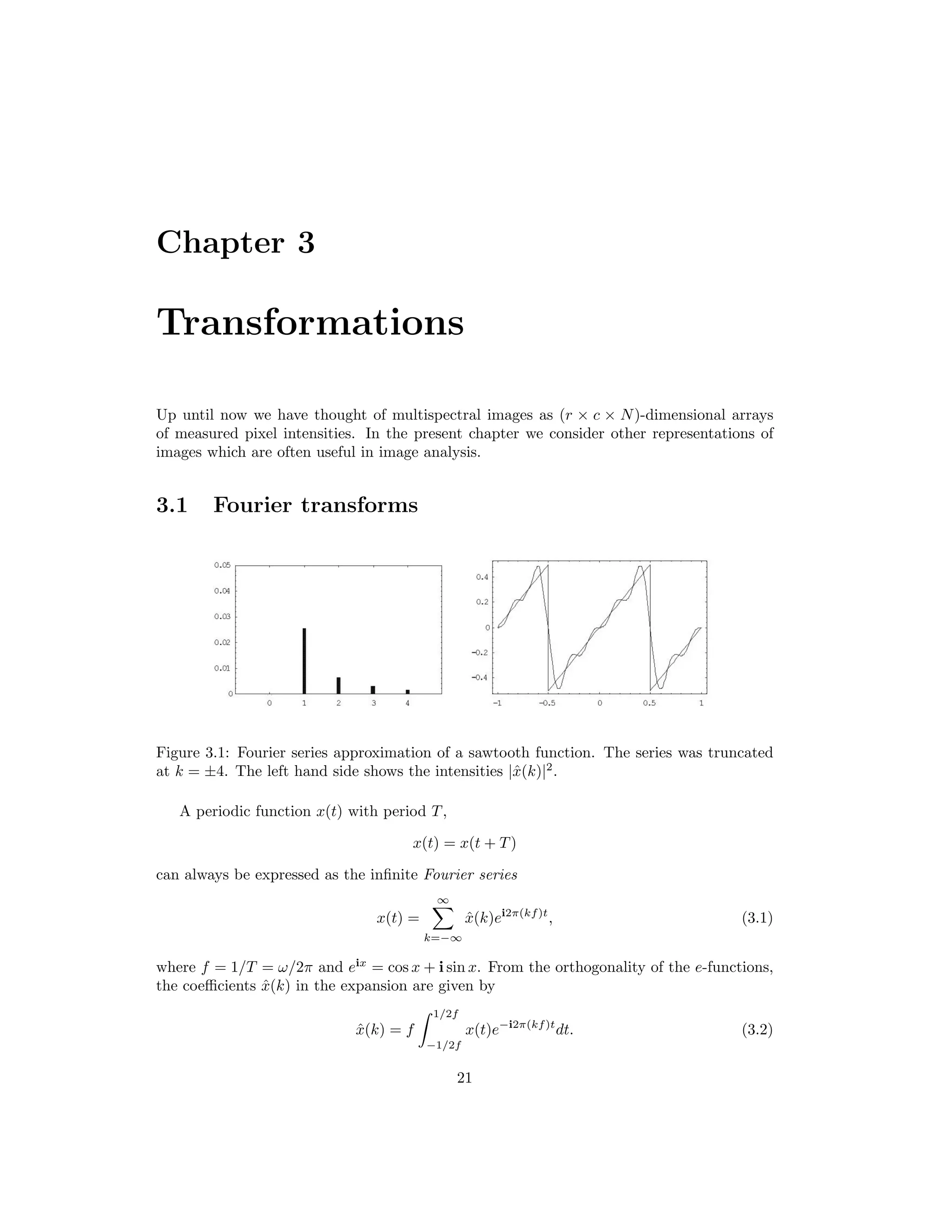
![3.2. WAVELETS 23 Thus we can write g(j) = 1 c c−1 k=0 ˆg(k)ei2πkj/c , j = 0 . . . c − 1, (3.4) if we interpret ˆg(k) → ˆg(k − c) when k ≥ c/2. The solution to (3.4) for the complex frequency components ˆg(k) is called the discrete Fourier transform and is given by ˆg(k) = c−1 j=0 g(j)e−i2πkj/c , k = 0 . . . c − 1. (3.5) This follows from the following orthogonality property: c−1 j=0 ei2π(k−k )j/c = cδk,k . (3.6) Eq. (3.4) itself is the discrete inverse Fourier transform. The discrete analog of Parsival’s formula is c−1 k=0 |ˆg(k)|2 = 1 c c−1 j=0 g(j)2 . (3.7) Determining the frequency components in (3.5) would appear to involve, in all, c2 floating point multiplication operations. The fast Fourier transform (FFT) exploits the structure of the complex e-functions to reduce this to order c log c, see for example [PFTV86]. 3.1.2 Discrete Fourier transform of an image The discrete Fourier transform is easily generalized to two dimensions for the purpose of image analysis. Let g(i, j), i, j = 0 . . . c − 1, represent a (quadratic) gray scale image. Its discrete Fourier transform is ˆg(k, ) = c−1 i=0 c−1 j=0 g(i, j)e−i2π(ik+j )/c (3.8) and the corresponding inverse transform is g(i, j) = 1 c2 c−1 k=0 c−1 =0 ˆg(k, )ei2π(ik+j )/c . (3.9) 3.2 Wavelets Unlike the Fourier transform, which represents a signal (array of pixel intensities) in terms of pure frequency functions, the wavelet transform expresses the signal in terms of functions which are restricted both in terms of frequency and spatial extent. In many applications, this turns out to be particularly efficient and useful. We’ll see an example of this in Chapter 7, where we discuss image fusion in more detail. The wavelet transform is discussed in Appendix B.](https://image.slidesharecdn.com/mortonjohncanty-imageanalysisandpatternrecognitionforremotesensingwithalgorithmsinenvi-idl-190425063306/75/Morton-john-canty-image-analysis-and-pattern-recognition-for-remote-sensing-with-algorithms-in-envi-idl-31-2048.jpg)
![24 CHAPTER 3. TRANSFORMATIONS 3.3 Principal components The principal components transformation forms linear combinations of multispectral pixel intensities which are mutually uncorrelated and which have maximum variance. We assume without loss of generality that G = 0, so that the covariance matrix of a multispectral image is is Σ = GG , and look for a linear combination Y = a G with maximum variance, subject to the normalization condition a a = 1. Since the covariance of Y is a Σa, this is equivalent to maximizing an unconstrained Lagrange function, see Section 1.4, L = a Σa − 2λ(a a − 1). The maximum of L occurs at that value of a for which ∂L ∂a = 0. Recalling the rules for vector differentiation, ∂L ∂a = 2Σa − 2λa = 0 which is the eigenvalue problem Σa = λa. Since Σ is real and symmetric, the eigenvectors are orthogonal (and normalized). Denote them a1 . . . aN for eigenvalues λ1 ≥ . . . ≥ λN . Define the matrix A = (a1 . . . aN ), AA = I, and let the the transformed principal component vector be Y = A G with covariance matrix Σ . Then we have Σ = YY = A GG A = A ΣA = Diag(λ1 . . . λN ) = λ1 0 · · · 0 0 λ2 · · · 0 ... ... ... ... 0 0 · · · λN =: Λ. The fraction of the total variance in the original multispectral image which is described by the first i principal components is λ1 + . . . + λi λ1 + . . . + λi + . . . + λN . If the original multispectral channels are highly correlated, as is usually the case, the first few principal components will account for a very high percentage of the variance the image. For example, a color composite of the first 3 principal components of a LANDSAT TM scene displays essentially all of the information contained in the 6 spectral components in one single image. Nevertheless, because of the approximation involved in the assumption of a normal distribution, higher order principal components may also contain significant information [JRR99]. The principal components transformation can be performed directly from the ENVI main menu. However the following IDL program illustrates the procedure in detail: ; Principal components analysis envi_select, title=’Choose multispectral image’, $](https://image.slidesharecdn.com/mortonjohncanty-imageanalysisandpatternrecognitionforremotesensingwithalgorithmsinenvi-idl-190425063306/75/Morton-john-canty-image-analysis-and-pattern-recognition-for-remote-sensing-with-algorithms-in-envi-idl-32-2048.jpg)
![3.4. MINIMUM NOISE FRACTION 25 fid=fid, dims=dims,pos=pos if (fid eq -1) then return num_cols = dims[2]+1 num_lines = dims[4]+1 num_pixels = (num_cols*num_lines) num_channels = n_elements(pos) image=intarr(num_channels,num_pixels) for i=0,num_channels-1 do begin temp=envi_get_data(fid=fid,dims=dims,pos=pos[i]) m = mean(temp) image[i,*]=temp-m endfor ; calculate the transformation matrix A sigma = correlate(image,/covariance,/double) lambda = eigenql(sigma,eigenvectors=A,/double) print,’Covariance matrix’ print, sigma print,’Eigenvalues’ print, lambda print,’Eigenvectors’ print, A ; transform the image image = image##transpose(A) ; reform to BSQ format PC_array = bytarr(num_cols,num_lines,num_channels) for i = 0,num_channels-1 do PC_array[*,*,i] = $ reform(image[i,*],num_cols,num_lines,/overwrite) ; output the result to memory envi_enter_data, PC_array end 3.4 Minimum noise fraction Principal components analysis maximizes variance. This doesn’t always lead to images of decreasing image quality (i.e. of increasing noise). The MNF transformation minimizes the noise content rather than maximizing variance, so, if this is the desired criterion, it is to be preferred over PCA. Suppose we can represent a gray scale image G with covariance matrix Σ and zero mean as a sum of uncorrelated signal and noise noise components G = S + N,](https://image.slidesharecdn.com/mortonjohncanty-imageanalysisandpatternrecognitionforremotesensingwithalgorithmsinenvi-idl-190425063306/75/Morton-john-canty-image-analysis-and-pattern-recognition-for-remote-sensing-with-algorithms-in-envi-idl-33-2048.jpg)
![26 CHAPTER 3. TRANSFORMATIONS both normally distributed, with covariance matrices ΣS and ΣN and zero mean. Then we have Σ = GG = (S + N)(S + N) = SS + NN , since noise and signal are uncorrelated, i.e. SN = NS = 0. Thus Σ = ΣS + ΣN . (3.10) Now let us seek a linear combination a G for which the signal to noise ratio SNR = var(a S) var(a N) = a ΣSa a ΣN a is maximized. From (3.10) we can write this in the form SNR = a Σa a ΣN a − 1. (3.11) Differentiating we get ∂ ∂a SNR = 1 a ΣN a 1 2 Σa − a Σa (a ΣN a)2 1 2 ΣN a = 0, or, equivalently, (a ΣN a)Σa = (a Σa)ΣN a . This condition is met when a solves the generalized eigenvalue problem ΣN a = λΣa. (3.12) Both ΣN and Σ are symmetric and the latter is also positive definite. Its Cholesky factor- ization is Σ = LL , where L is a lower triangular matrix, and can be thought of as the “square root” of Σ. Such an L always exists is Σ is positive definite. With this, we can write (3.12) as ΣN a = λLL a or, equivalently, L−1 ΣN (L )−1 L a = λL a or, with b = L a and commutivity of inverse and transpose, [L−1 ΣN (L−1 ) ]b = λb, a standard eigenproblem for a real, symmetric matrix L−1 ΣN (L−1 ) . From (3.11) we see that the SNR for eigenvalue λi is just SNRi = ai Σai ai (λiΣai) − 1 = 1 λi − 1. Thus the eigenvector ai corresponding to the smallest eigenvalue λi will maximize the signal to noise ratio. Note that (3.12) can be written in the form ΣN A = ΣAΛ, (3.13)](https://image.slidesharecdn.com/mortonjohncanty-imageanalysisandpatternrecognitionforremotesensingwithalgorithmsinenvi-idl-190425063306/75/Morton-john-canty-image-analysis-and-pattern-recognition-for-remote-sensing-with-algorithms-in-envi-idl-34-2048.jpg)
![3.5. MAXIMUM AUTOCORRELATION FACTOR (MAF) 29 Differentiating, ∂R ∂a = 1 a Σa 1 2 Σ∆a − a Σ∆a (a Σa)2 1 2 Σa = 0 or (a Σa)Σ∆a = (a Σ∆a)Σa. This condition is met when a solves the generalized eigenvalue problem Σ∆a = λΣa, (3.18) which is seen to have the same form as (3.12). Again both Σ∆ and Σ are symmetric and the latter is also positive definite and we obtain the standard eigenproblem [L−1 Σ∆(L−1 ) ]b = λb, for the real, symmetric matrix L−1 Σ∆(L−1 ) . Let the eigenvalues be λ1 ≥ . . . λN and the corresponding (orthogonal) eigenvectors be bi. We have 0 = bi bj = ai LL aj = ai Σaj, i = j, and therefore cov(ai G(x), aj G(x)) = ai Σaj = 0, i = j, so that the MAF components are orthogonal (uncorrelated). Moreover with equation (2.14) we have corr(ai G(x), ai G(x + ∆)) = 1 − 1 2 λi, and the first MAF component has minimum autocorrelation. An ENVI plug-in for performing the MAF transformation is given in Ap- pendix D.5.2.](https://image.slidesharecdn.com/mortonjohncanty-imageanalysisandpatternrecognitionforremotesensingwithalgorithmsinenvi-idl-190425063306/75/Morton-john-canty-image-analysis-and-pattern-recognition-for-remote-sensing-with-algorithms-in-envi-idl-37-2048.jpg)
![30 CHAPTER 3. TRANSFORMATIONS Exercises 1. Show that, for x(t) = sin(2πt) in Eq. (2.2), ˆx(−1) = − 1 2i , ˆx(1) = 1 2i , and ˆx(k) = 0 otherwise. 2. Calculate the discrete Fourier transform of the sequence 2, 4, 6, 8 from (3.4). You have to solve four simultaneous equations, the first of which is 2 = 1 4 ˆg(0) + ˆg(1) + ˆg(2) + ˆg(3) . Verify your result in IDL with the command print, FFT([2,4,6,8])](https://image.slidesharecdn.com/mortonjohncanty-imageanalysisandpatternrecognitionforremotesensingwithalgorithmsinenvi-idl-190425063306/75/Morton-john-canty-image-analysis-and-pattern-recognition-for-remote-sensing-with-algorithms-in-envi-idl-38-2048.jpg)
![Chapter 4 Radiometric enhancement 4.1 Lookup tables Figure 4.1: Contrast enhancement with a lookup table represented as the continuous function f(x) [JRR99]. Intensity enhancement of an image is easily accomplished by means of lookup tables. For byte-encoded data, the pixel intensities g are used to index an array LUT[k], k = 0 . . . 255, the entries of which also lie between 0 and 255. These entries can be chosen to implement linear stretching, saturation, histogram equalization, etc. according to ˆgk(i, j) = LUT[gk(i, j)], 0 ≤ i ≤ r − 1, 0 ≤ j ≤ c − 1. 31](https://image.slidesharecdn.com/mortonjohncanty-imageanalysisandpatternrecognitionforremotesensingwithalgorithmsinenvi-idl-190425063306/75/Morton-john-canty-image-analysis-and-pattern-recognition-for-remote-sensing-with-algorithms-in-envi-idl-39-2048.jpg)
![32 CHAPTER 4. RADIOMETRIC ENHANCEMENT It is also useful to think of the the lookup table as an approximately continuous function y = f(x). If hin(x) is the histogram of the original image and hout(y) is the histogram of the image after transformation through the lookup table, then, since the number of pixels is constant, hout(y) dy = hin(x) dx, see Fig.4.1 4.1.1 Histogram equalization For histogram equalization, we want hout(y) to be constant independent of y. Hence dy ∼ hin(x) dx and y = f(x) ∼ x 0 hin(t)dt. The lookup table y for histogram equalization is thus proportional to the cumulative sum of the original histogram. 4.1.2 Histogram matching Figure 4.2: Steps required for histogram matching [JRR99]. It is often desirable to match the histogram of one image to that of another so as to make their apparent brightnesses as similar as possible, for example when the two images](https://image.slidesharecdn.com/mortonjohncanty-imageanalysisandpatternrecognitionforremotesensingwithalgorithmsinenvi-idl-190425063306/75/Morton-john-canty-image-analysis-and-pattern-recognition-for-remote-sensing-with-algorithms-in-envi-idl-40-2048.jpg)
![4.2. CONVOLUTIONS 33 are combined in a mosaic. We can do this by first equalizing both the input histogram hin(x) and the reference histogram href (y) with the cumulative lookup tables z = f(x) and z = g(y), respectively. The required lookup table is then y = g−1 (z) = g−1 (f(x)). The necessary steps for implementing this function are illustrated in Fig. 1.5 taken from [JRR99]. 4.2 Convolutions With the convention ω = 2πk/c we can write (3.5) in the form ˆg(ω) = c−1 j=0 g(j)e−iωj . (4.1) The convolution of g with a filter h = (h(0), h(1), . . .) is defined by f(j) = k h(k)g(j − k) =: h ∗ g, (4.2) where the sum is over all nonzero elements of the filter h. If the number of nonzero elements is finite, we speak of a finite impulse response filter (FIR). Theorem 1 (Convolution theorem) In the frequency domain, convolution is replaced by multiplication: ˆf(ω) = ˆh(ω)ˆg(ω). Proof: ˆf(ω) = j f(j)e−iωj = j,k h(k)g(j − k)e−iωj ˆh(ω)ˆg(ω) = k h(k)e−iωk g( )e−iω = k, h(k)g( )e−iω(k+ ) = k,j h(k)g(j − k)e−iωj = ˆf(ω). This can of course be generalized to two dimensional images, so that there are three basic steps involved in image filtering: 1. The image and the convolution filter are transformed from the spatial domain to the frequency domain using the FFT. 2. The transformed image is multiplied with the frequency filter. 3. The filtered image is transformed back to the spatial domain.](https://image.slidesharecdn.com/mortonjohncanty-imageanalysisandpatternrecognitionforremotesensingwithalgorithmsinenvi-idl-190425063306/75/Morton-john-canty-image-analysis-and-pattern-recognition-for-remote-sensing-with-algorithms-in-envi-idl-41-2048.jpg)
![34 CHAPTER 4. RADIOMETRIC ENHANCEMENT We often distinguish between low-pass and high-pass filters. Low pass filters perform some sort of averaging. The simplest example is h = (1/2, 1/2, 0 . . .), which computes the average of two consecutive pixels. A high-pass filter computes differences of nearby pixels, e.g. h = (1/2, −1/2, 0 . . .). Figure 4.3 shows the Fourier transforms of these two simple filters generated by the the IDL program ; Hi-Lo pass filters x = fltarr(64) x[0]=0.5 x[1]=-0.5 p1 =abs(FFT(x)) x[1]=0.5 p2 =abs(FFT(x)) envi_plot_data,lindgen(64),[[p1],[p2]] end Figure 4.3: Low-pass(red) and high-pass (white) filters in the frequency domain. The quan- tity |ˆh(k)|2 is plotted as a function of k. The highest frequency is at the center of the plots, k = c/2 = 32 . 4.2.1 Laplacian of Gaussian filter We shall illustrate image filtering with the so-called Laplacian of Gaussian (LoG) filter, which will be used in Chapter 6 to implement contour matching for automatic determination of ground control points. To begin with, consider the gradient operator for a two-dimensional image: = ∂ ∂x = i ∂ ∂x1 + j ∂ ∂x2 ,](https://image.slidesharecdn.com/mortonjohncanty-imageanalysisandpatternrecognitionforremotesensingwithalgorithmsinenvi-idl-190425063306/75/Morton-john-canty-image-analysis-and-pattern-recognition-for-remote-sensing-with-algorithms-in-envi-idl-42-2048.jpg)
![4.2. CONVOLUTIONS 35 where i and j are unit vectors in the vertical and horizontal directions, respectively. g(x) is a vector in the direction of the maximum rate of change of gray scale intensity. Since the intensity values are discrete, the partial derivatives must be approximated. For example we can use the Sobel operators: ∂g(x) ∂x1 ≈ [g(i − 1, j − 1) + 2g(i, j − 1) + g(i + 1, j − 1)] − [g(i − 1, j + 1) + 2g(i, j + 1) + g(i + 1, j + 1)] = 2(i, j) ∂g(x) ∂x2 ≈ [g(i − 1, j − 1) + 2g(i − 1, j) + g(i − 1, j + 1)] − [g(i + 1, j − 1) + 2g(i + 1, j) + g(i + 1, j + 1)] = 1(i, j) which are equivalent to the two-dimensional FIR filters h1 = −1 0 1 −2 0 2 −1 0 1 and h2 = 1 2 1 0 0 0 −1 −2 −1 , respectively. The magnitude of the gradient is | | = 2 1 + 2 2. Edge detection can be achieved by calculating the filtered image f(i, j) = | |(i, j) and setting an appropriate threshold. Figure 4.4: Laplacian of Gaussian filter.](https://image.slidesharecdn.com/mortonjohncanty-imageanalysisandpatternrecognitionforremotesensingwithalgorithmsinenvi-idl-190425063306/75/Morton-john-canty-image-analysis-and-pattern-recognition-for-remote-sensing-with-algorithms-in-envi-idl-43-2048.jpg)
![36 CHAPTER 4. RADIOMETRIC ENHANCEMENT Now consider the second derivatives of the image intensities, which can be represented formally by the Laplacian 2 = · = ∂2 ∂x2 1 + ∂2 ∂x2 2 . 2 g(x) is a scalar quantity which is zero whenever the gradient is maximum. Therefore changes in intensity from dark to light or vice versa correspond to sign changes in the Laplacian and these can also be used for edge detection. The Laplacian can also be ap- proximated by a FIR filter, however such filters tend to be very sensitive to image noise. Usually a low-pass Gauss filter is first used to smooth the image before the Laplacian filter is applied. It is more efficient, however, to calculate the Laplacian of the Gauss function itself and then use the resulting function to derive a high-pass filter. The Gauss function in two dimensions is given by 1 2πσ2 exp − 1 2σ2 (x2 1 + x2 2), where the parameter σ determines its extent. Its Laplacian is 1 2πσ6 (x2 1 + x2 2 − 2σ2 ) exp − 1 2σ2 (x2 1 + x2 2) a plot of which is shown in Fig. 4.4. The following program illustrates the application of the filter to a gray scale image, see Fig. 4.5: pro LoG sigma = 2.0 filter = fltarr(17,17) for i=0L,16 do for j=0L,16 do $ filter[i,j] = (1/(2*!pi*sigma^6))*((i-8)^2+(j-8)^2-2*sigma^2) $ *exp(-((i-8)^2+(j-8)^2)/(2*sigma^2)) ; output as EPS file thisDevice =!D.Name set_plot, ’PS’ Device, Filename=’c:tempLoG.eps’,xsize=4,ysize=4,/inches,/Encapsulated shade_surf,filter device,/close_file set_plot, thisDevice ; read a jpg image filename = Dialog_Pickfile(Filter=’*.jpg’,/Read) OK = Query_JPEG(filename,fileinfo) if not OK then return xsize = fileinfo.dimensions[0] ysize = fileinfo.dimensions[1] window,11,xsize=xsize,ysize=ysize Read_JPEG,filename,image1 image = bytarr(xsize,ysize)](https://image.slidesharecdn.com/mortonjohncanty-imageanalysisandpatternrecognitionforremotesensingwithalgorithmsinenvi-idl-190425063306/75/Morton-john-canty-image-analysis-and-pattern-recognition-for-remote-sensing-with-algorithms-in-envi-idl-44-2048.jpg)
![4.2. CONVOLUTIONS 37 image[*,*] = image1[0,*,*] tvscl,image ; run the filter filt = image*0.0 filt[0:16,0:16]=filter[*,*] image1= float(fft(fft(image)*fft(filt),1)) ; get zero-crossings and display image2 = bytarr(xsize,ysize) indices = where( (image1*shift(image1,1,0) lt 0) or (image1*shift(image1,0,1) lt 0) ) image2[indices]=255 wset, 11 tv, image2 end Figure 4.5: Image filtered with the Laplacian of Gaussian filter.](https://image.slidesharecdn.com/mortonjohncanty-imageanalysisandpatternrecognitionforremotesensingwithalgorithmsinenvi-idl-190425063306/75/Morton-john-canty-image-analysis-and-pattern-recognition-for-remote-sensing-with-algorithms-in-envi-idl-45-2048.jpg)

![Chapter 5 Topographic modelling Satellite images are two-dimensional representations of the three-dimensional earth surface. The correct treatment of the third dimension – the elevation – is essential for terrain mod- elling and accurate georeferencing. 5.1 RST transformation Transformations of spatial coordinates1 in 3 dimensions which involve only rotations, scaling and translations can be represented by a 4 × 4 transformation matrix A v∗ = Av (5.1) where v is the column vector containing the original coordinates v = (X, Y, Z, 1) and v∗ contains the transformed coordinates v∗ = (X∗ , Y ∗ , Z∗ , 1) . For example the translation X∗ = X + X0 Y ∗ = Y + Y0 Z∗ = Z + Z0 corresponds to the transformation matrix T = 1 0 0 X0 0 1 0 Y0 0 0 1 Z0 0 0 0 1 , a uniform scaling by 50% to S = 1/2 0 0 0 0 1/2 0 0 0 0 1/2 0 0 0 0 1 , 1The following treatment closely follows Chapter 2 of Gonzales and Woods [GW02]. 39](https://image.slidesharecdn.com/mortonjohncanty-imageanalysisandpatternrecognitionforremotesensingwithalgorithmsinenvi-idl-190425063306/75/Morton-john-canty-image-analysis-and-pattern-recognition-for-remote-sensing-with-algorithms-in-envi-idl-47-2048.jpg)
![40 CHAPTER 5. TOPOGRAPHIC MODELLING and a simple rotation θ about the Z-axis to Rθ = cos θ sin θ 0 0 −sinθ cosθ 0 0 0 0 1 0 0 0 0 1 , etc. The complete RST transformation is then v∗ = RSTv = Av. (5.2) The inverse transformation is of course represented by A−1 . 5.2 Imaging transformations An imaging (or perspective) transformation projects 3D points onto a plane. It is used to describe the formation of a camera image and, unlike the RST transformation, is non-linear since it involves division by coordinate values. Figure 5.1: Basic imaging process, from [GW02]. In Figure 5.1, the camera coordinate system (x, y, x) is aligned with the world coordinate system, describing the terrain to be imaged. The camera focal length is λ. From sim- ple geometry we obtain expressions for the image plane coordinates in terms of the world coordinates: x = λX λ − Z y = λY λ − Z . (5.3) Solving for the X and Y world coordinates: X = x λ (λ − Z) Y = y λ (λ − Z). (5.4)](https://image.slidesharecdn.com/mortonjohncanty-imageanalysisandpatternrecognitionforremotesensingwithalgorithmsinenvi-idl-190425063306/75/Morton-john-canty-image-analysis-and-pattern-recognition-for-remote-sensing-with-algorithms-in-envi-idl-48-2048.jpg)
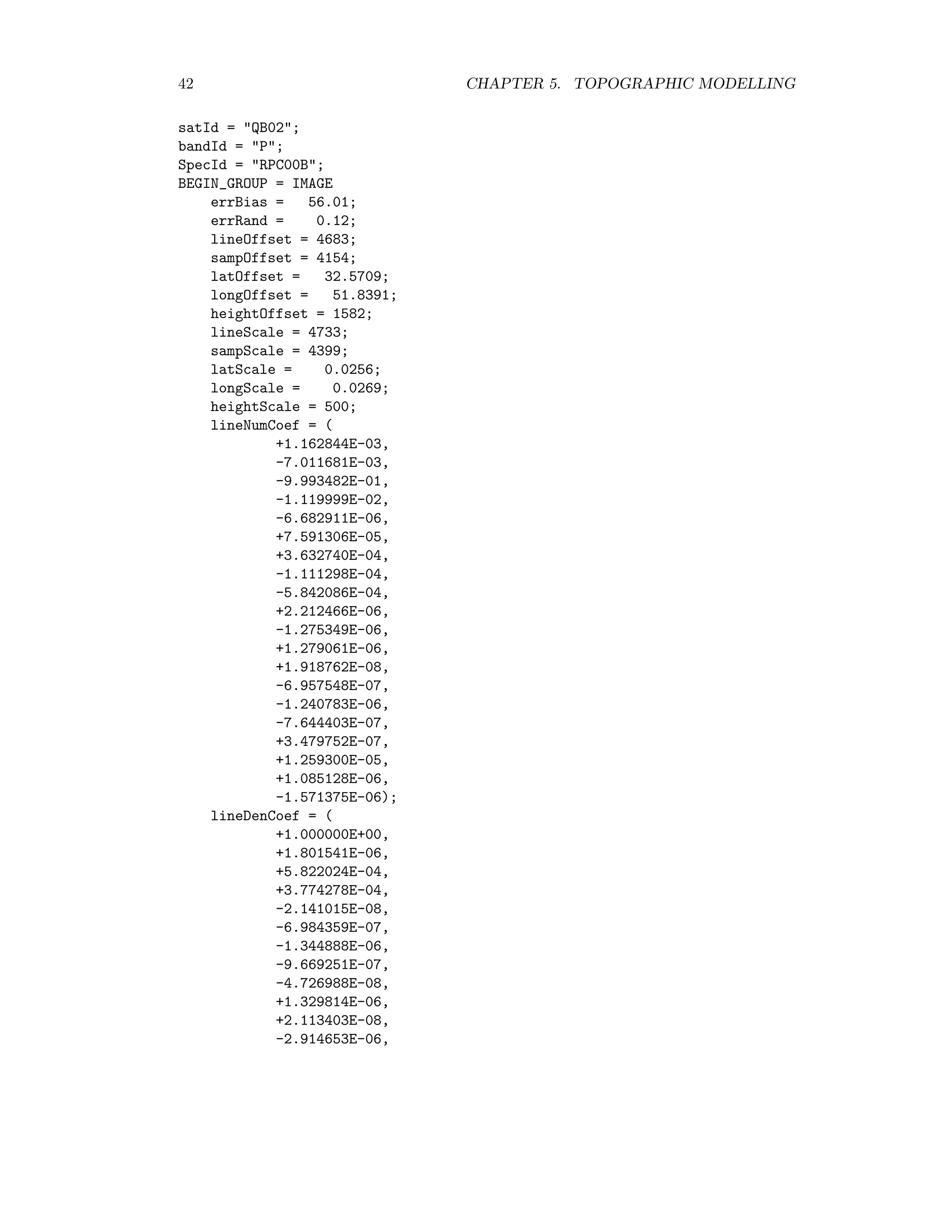
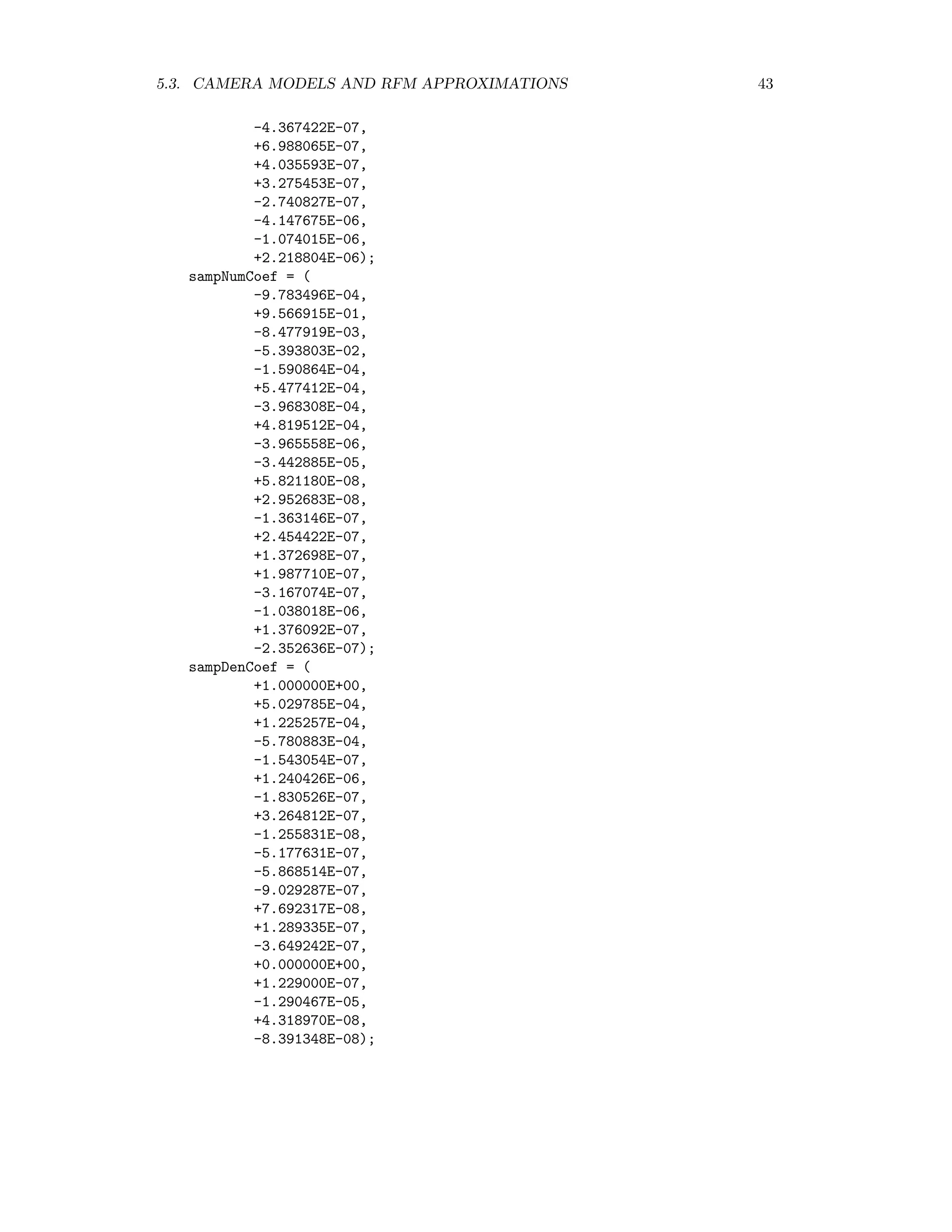
![5.3. CAMERA MODELS AND RFM APPROXIMATIONS 41 Thus, in order to extract the geographical coordinates (X, Y ) of a point on the earth’s surface from its image coordinates, we require knowledge of the elevation Z. Correcting for the elevation in this way constitutes the process of orthorectification. 5.3 Camera models and RFM approximations Equation (5.3) is overly simplified, as it assumes that the origin of world and image coordi- nates coincide. In order to apply it, one has first to transform the image coordinate system from the satellite to the world coordinate system. This is done in a straightforward way with the rotation and translation transformations introduced in Section 5.1. However it requires accurate knowledge of the height and orientation of the satellite imaging system at the time of the image acquisition (or, more exactly, during the acquisition, since the latter is normally not instantaneous). The resulting non-linear equations that relate image and world coordinates are what constitute the camera or sensor model for that particular image. Direct use of the camera model for image processing is complicated as it requires ex- tremely exact, sometimes proprietary information about the sensor system and its orbit. An alternative exists if the image provider also supplies a so-called rational function model (RFM) which approximates the camera model for each acquisition as a ratio of rational polynomials, see e.g. [TH01]. Such RFMs have the form r = f(X , Y , Z ) = a(X , Y , Z ) b(X , Y , Z ) c = g(X , Y , Z ) = c(X , Y , Z ) d(X , Y , Z ) (5.5) where c and r are the column and row (XY) coordinates in the image plane relative to an origin (c0, r0) and scaled by a factor cs resp. rs: c = c − c0 cs , r = r − r0 rs . Similarly X , Y and Z are relative, scaled world coordinates: X = X − X0 Xs , Y = Y − Y0 Ys , Z = Z − Z0 Zs . The polynomials a, b, c and d are typically to third order in the world coordinates, e.g. a(X, Y, Z) = a0 + a1X + a2Y + a3Z + a4XY + a5XZ + a6Y Z + a7X2 + a8Y 2 + a9Z2 + a10XY Z + a11X3 + a12XY 2 + a13XZ2 + a14X2 Y + a15Y 3 + a16Y Z2 + a17X2 Z + a18Y 2 Z + a19Z3 The advantage of using ratios of polynomials is that these are less subject to interpolation error. For a given acquisition the provider fits the RFM to his camera model using a three- dimensional grid of points covering the image and world spaces with a least squares fitting procedure. The RFM is capable of representing the camera model extremely well and can be used as a replacement for it. Both Space Imaging and Digital Globe provide RFMs with their high resolution IKONOS and QuickBird imagery. Below is a sample Quickbird RFM file giving the origins, scaling factors and polynomial coefficients needed in Eq. (5.5).](https://image.slidesharecdn.com/mortonjohncanty-imageanalysisandpatternrecognitionforremotesensingwithalgorithmsinenvi-idl-190425063306/75/Morton-john-canty-image-analysis-and-pattern-recognition-for-remote-sensing-with-algorithms-in-envi-idl-49-2048.jpg)
![5.4. STEREO IMAGING, ELEVATION MODELS AND ORTHORECTIFICATION 45 Figure 5.2: The stereo imaging process, from [GW02]. Figure 5.3: Top view of Figure 5.2, from [GW02].](https://image.slidesharecdn.com/mortonjohncanty-imageanalysisandpatternrecognitionforremotesensingwithalgorithmsinenvi-idl-190425063306/75/Morton-john-canty-image-analysis-and-pattern-recognition-for-remote-sensing-with-algorithms-in-envi-idl-53-2048.jpg)
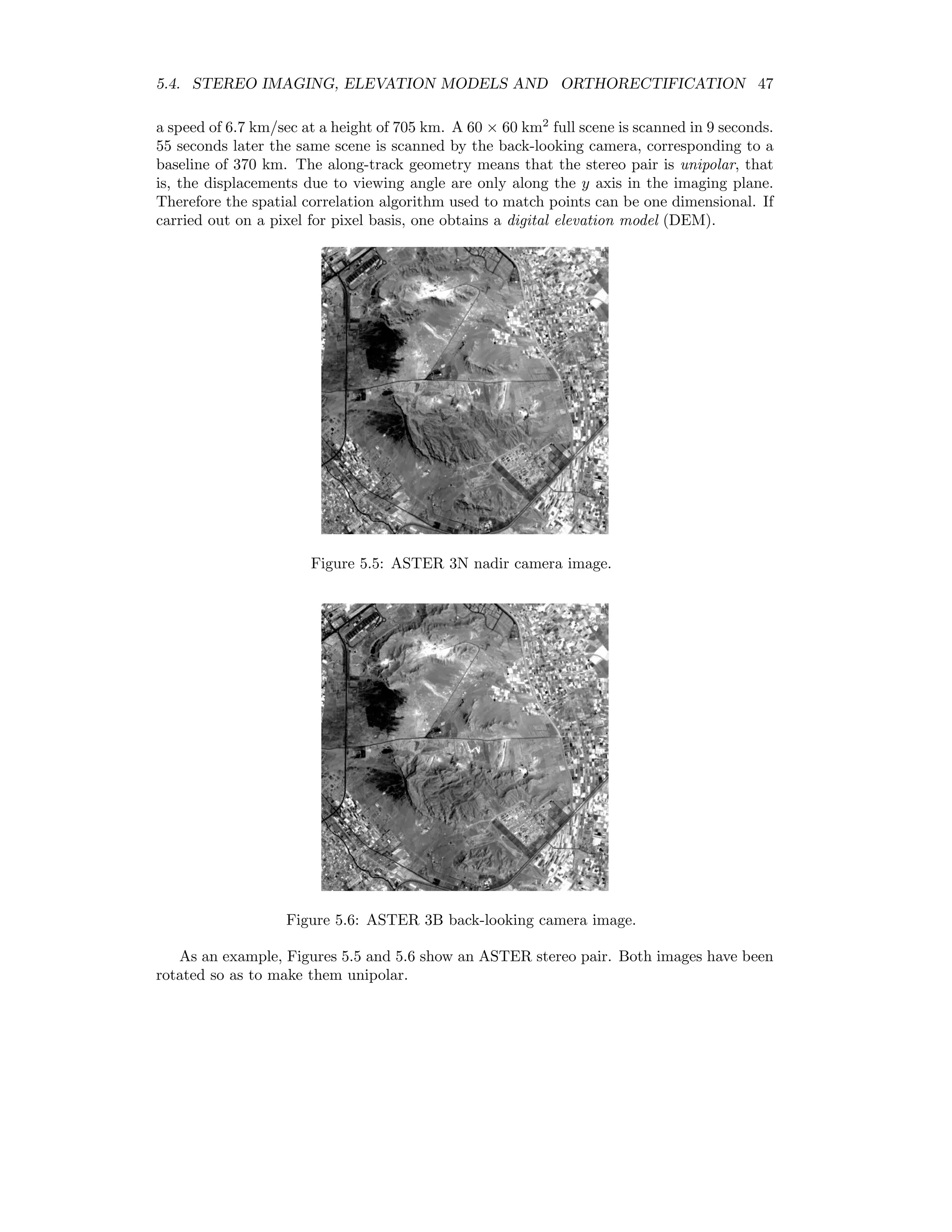
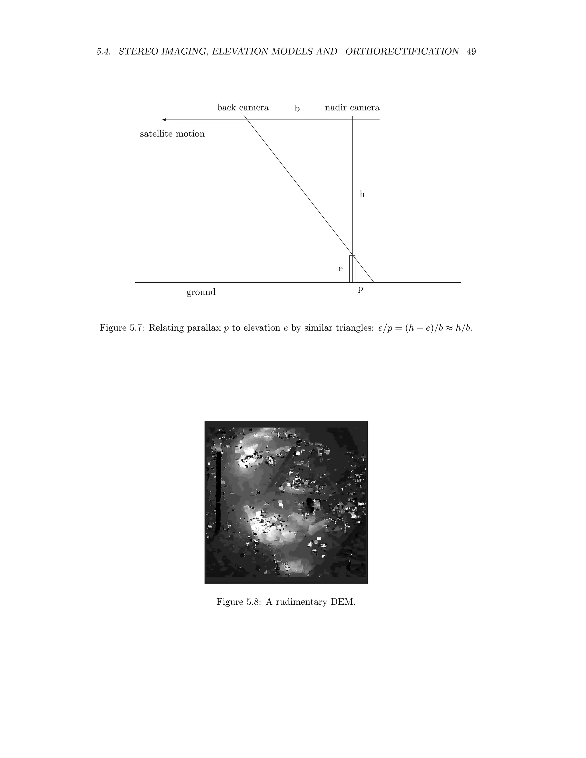
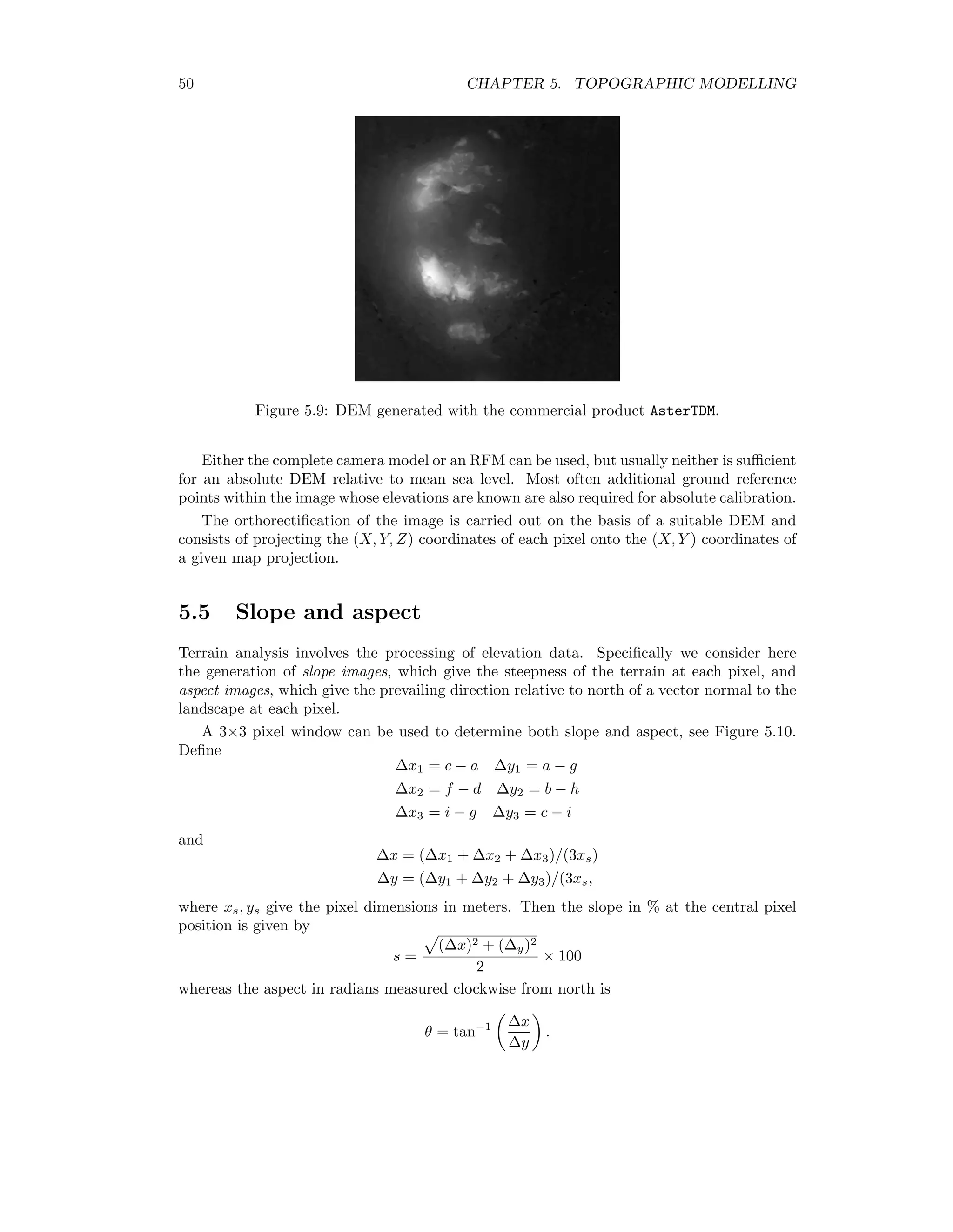
![48 CHAPTER 5. TOPOGRAPHIC MODELLING The following IDL program calculates a very rudimentary DEM: pro test_correl_images height = 705.0 base = 370.0 pixel_size = 15.0 envi_select, title=’Choose 1st image’, fid=fid1, dims=dims1, pos=pos1, /band_only envi_select, title=’Choose 2nd image’, fid=fid2, dims=dims2, pos=pos2, /band_only im1 = envi_get_data(fid=fid1,dims=dims1,pos=pos1) im2 = envi_get_data(fid=fid2,dims=dims2,pos=pos2) n_cols = dims1[2]-dims1[1]+1 n_rows = dims1[4]-dims1[3]+1 parallax = fltarr(n_cols,n_rows) progressbar = Obj_New(’progressbar’, Color=’blue’, Text=’0’,$ title=’Cross correlation, column ...’,xsize=250,ysize=20) progressbar-start for i=7L,n_cols-8 do begin if progressbar-CheckCancel() then begin envi_enter_data,pixel_size*parallax*(height/base) progressbar-Destroy return endif progressbar-Update,(i*100)/n_cols,text=strtrim(i,2) for j=25L,n_rows-26 do begin cim = correl_images(im1[i-5:i+5,j-5:j+5],im2[i-7:i+7,j-25:j+25], $ xoffset_b=0,yoffset_b=-20,xshift=0,yshift=20) corrmat_analyze,cim,xoff,yoff,m,e,p parallax[i,j] = yoff (-5.0) endfor endfor progressbar-destroy envi_enter_data,pixel_size*parallax*(height/base) end This program makes use of the routines correl images and corrmat analyze from the IDL Astronomy User’s Library2 to calculate the cross-correlation of the two images. For each pixel in the nadir image an 11 × 11 window is moved along an 11 × 51 window in the back- looking image centered at the same position. The point of maximum correlation defines the parallax or displacement p. This is related to the relative elevation e of the pixel according to e = h b p × 15m, where h is the height of the sensor and b is the baseline, see Figure 5.7. Figure 5.8 shows the result. Clearly there are many problems due to the correlation errors, however the relative elevations are approximately correct when compared to the DEM determined with the ENVI commercial add-on AsterDTM, see Figure 5.9. 2www.astro.washington.edu/deutsch/idl/htmlhelp/index.html](https://image.slidesharecdn.com/mortonjohncanty-imageanalysisandpatternrecognitionforremotesensingwithalgorithmsinenvi-idl-190425063306/75/Morton-john-canty-image-analysis-and-pattern-recognition-for-remote-sensing-with-algorithms-in-envi-idl-56-2048.jpg)
![5.6. ILLUMINATION CORRECTION 51 a b c d e f g h i Figure 5.10: Pixel elevations in an 8-neighborhood. The letters represent elevations. Slope/aspect determinations from a DEM are available in the ENVI main menu under Topographic/Topographic Modelling. 5.6 Illumination correction Figure 5.11: Angles involved in computation of local solar elevation, taken from [RCSA03]. Topographic modelling can be used to correct images for the effects of local solar illu- mination, which depends not only upon the sun’s position (elevation and azimuth) but also upon the local slope and aspect of the terrain being illuminated. Figure 5.11 shows the angles involved [RCSA03]. Solar elevation is θi, solar azimuth is φa, θp is the slope and φ0 is the aspect. The quantity to be calculated is the local solar elevation γi which determines](https://image.slidesharecdn.com/mortonjohncanty-imageanalysisandpatternrecognitionforremotesensingwithalgorithmsinenvi-idl-190425063306/75/Morton-john-canty-image-analysis-and-pattern-recognition-for-remote-sensing-with-algorithms-in-envi-idl-59-2048.jpg)
![52 CHAPTER 5. TOPOGRAPHIC MODELLING the local irradiance. From trigonometry we have cos γi = cos θp cos θi + sin θp sin θi cos(φa − φ0). (5.8) An example of a cos γi image in hilly terrain is shown in Figure 5.12. Figure 5.12: Cosine of local solar illumination angle stretched across a DEM. Let ρT represent the reflectance of the inclined surface in Figure 5.11. Then for a Lambertian surface, i.e. a surface which scatters reflected radiation uniformly in al directions, the reflectance of the corresponding horizontal surface ρH would be ρH = ρT cos θi cos γi . (5.9) The Lambertian assumption is in general not correct, the actual reflectance being de- scribed by a complicated bidirectional reflectance distribution function (BRDF). An empiri- cal appraoch which gives a better approximation to the BRDF is the C-correction [TGG82]. Let m and b be the slope and intercept of a regression line for reflectance vs. cos γi for a particular image band. Then instead of (5.9) one uses ρH = ρT cosθi + b/m cos γi + b/m . (5.10) An ENVI plug-in for illumination correction with the C-correction approxi- mation is given in Appendix D.2.2.](https://image.slidesharecdn.com/mortonjohncanty-imageanalysisandpatternrecognitionforremotesensingwithalgorithmsinenvi-idl-190425063306/75/Morton-john-canty-image-analysis-and-pattern-recognition-for-remote-sensing-with-algorithms-in-envi-idl-60-2048.jpg)
![Chapter 6 Image Registration Image registration, either to another image or to a map, is a fundamental task in image processing. It is required for georeferencing, stereo imaging, accurate change detection, or any kind of multitemporal image analysis. Image-to-image registration methods can be divided into roughly four classes [RC96]: 1. algorithms that use pixel values directly, i.e. correlation methods 2. frequency- or wavelet-domain methods that use e.g. the fast fourier transform(FFT) 3. feature-based methods that use low-level features such as edges and corners 4. algorithms that use high level features and the relations between them, e.g. object- oriented methods We consider examples of frequency-domain and feature-based methods here. 6.1 Frequency domain registration Consider two N × N gray scale images g1(i , j ) and g2(i, j), where g2 is offset relative to g1 by an integer number of pixels: g2(i, j) = g1(i , j ) = g1(i − i0, j − j0), i0, j0 N. Taking the Fourier transform we have ˆg2(k, l) = ij g1(i − i0, j − j0)e−i2π(ik+jl)/N , or with a change of indices to i j , ˆg2(k, l) = i j g1(i , j )e−i2π(i k+j l)/N e−i2π(i0k+j0l)/N = ˆg1(k, l)e−i2π(i0k+j0l)/N . (This is referred to as the Fourier translation property.) Therefore we can write ˆg2(k, l)ˆg∗ 1(k, l) |ˆg2(k, l)ˆg∗ 1(k, l)| = e−i2π(i0k+j0l)/N , (6.1) 53](https://image.slidesharecdn.com/mortonjohncanty-imageanalysisandpatternrecognitionforremotesensingwithalgorithmsinenvi-idl-190425063306/75/Morton-john-canty-image-analysis-and-pattern-recognition-for-remote-sensing-with-algorithms-in-envi-idl-61-2048.jpg)
![54 CHAPTER 6. IMAGE REGISTRATION Figure 6.1: Phase correlation of two identical images shifted by 10 pixels. where ˆg∗ 1 is the complex conjugate of ˆg1. The inverse transform of the right hand side exhibits a Dirac delta function (spike) at the coordinates (i0, j0). Thus if two otherwise identical images are offset by an integer number of pixels, the offset can be found by taking their Fourier transforms, computing the ratio on the left hand side of (6.1) (the so-called cross-power spectrum) and then taking the inverse transform of the result. The position of the maximum value in the inverse transform gives the values of i0 and j0. The following IDL program illustrates the procedure, see Fig. 6.1 ; Image matching by phase correlation ; read a bitmap image and cut out two 512x512 pixel arrays filename = Dialog_Pickfile(Filter=’*.jpg’,/Read) if filename eq ’’ then print, ’cancelled’ else begin Read_JPeG,filename,image g1 = image[0,10:521,10:521] g2 = image[0,0:511,0:511] ; perform Fourier transforms f1 = fft(g1, /double) f2 = fft(g2, /double) ; Determine the offset g = fft( f2*conj(f1)/abs(f1*conj(f1)), /inverse, /double )](https://image.slidesharecdn.com/mortonjohncanty-imageanalysisandpatternrecognitionforremotesensingwithalgorithmsinenvi-idl-190425063306/75/Morton-john-canty-image-analysis-and-pattern-recognition-for-remote-sensing-with-algorithms-in-envi-idl-62-2048.jpg)
![6.2. FEATURE MATCHING 55 pos = where(g eq max(g)) print, ’Offset = ’ + strtrim(pos mod 512) + strtrim(pos/512) ; output as EPS file thisDevice =!D.Name set_plot, ’PS’ Device, Filename=’c:tempphasecorr.eps’,xsize=4,ysize=4,/inches,/Encapsulated shade_surf,g[0,0:50,0:50] device,/close_file set_plot, thisDevice endelse end Images which differ not only by an offset but also by a rigid rotation and change of scale can in principle be registered similarly, see [RC96]. 6.2 Feature matching A tedious task associated with image-image registration using low level image features is the setting of ground control points (GCPs) since, in general, it is necessary to resort to the manual entry. However various techniques for automatic determination of GCPs have been suggested in the literature. We will discuss one such method, namely contour matching [LMM95]. This technique has been found to function reliably in bitemporal scenes in which vegetation changes do not dominate. It can of course be augmented (or replaced) by other automatic methods or by manual determination. The procedures involved in image-image registration using contour matching are shown in Fig. 6.2 [LMM95]. LoG Zero Crossing Edge Strength Contour Finder Chain Code Encoder Closed Contour Matching Consistency Check Warping E E E E E E cc ''' Image 1 Image 2 Image 2 (registered) Figure 6.2: Image-image registration with contour matching.](https://image.slidesharecdn.com/mortonjohncanty-imageanalysisandpatternrecognitionforremotesensingwithalgorithmsinenvi-idl-190425063306/75/Morton-john-canty-image-analysis-and-pattern-recognition-for-remote-sensing-with-algorithms-in-envi-idl-63-2048.jpg)
![56 CHAPTER 6. IMAGE REGISTRATION 6.2.1 Contour detection The first step involves the application of a Laplacian of Gaussian filter to both images. After determining the contours by examining zero-crossings of the LoG-filtered image, the contour strengths are encoded in the pixel intensities. Strengths are taken to be proportional to the magnitude of the gradient at the zero-crossing. 6.2.2 Closed contours In the next step, all closed contours with strengths above some given threshold are deter- mined by tracing the contours. Pixels which have been visited during tracing are set to zero so that they will not be visited again. 6.2.3 Chain codes For subsequent matching purposes, all significant closed contours found in the preceding step are chain encoded. Any digital curve can be represented by an integer sequence {a1, a2 . . . ai . . .}, ai ∈ {0, 1, 2, 3, 4, 5, 6, 7}, depending on the relative position of the current pixel with respect to the previous pixel in the curve. This simple code has the drawback that some contours produce wrap around. For example the line in the direction −22.5o has the chain code {707070 . . .}. Li et al. [LMM95] suggest the smoothing operation: {a1a2 . . . an} → {b1b2 . . . bn}, where b1 = a1 and bi = qi, qi is an integer satisfying (qi−ai) mod 8 = 0 and |qi−bi−1| → min, i = 2, 3 . . . n. They also suggest the applying the Gaussian smoothing filter {0.1, 0.2, 0.4, 0.2, 0.1} to the result. Two chain codes can be compared by “sliding” one over the other and determining the maximum correlation between them. 6.2.4 Invariant moments The closed contours are first matched according to their invariant moments. These are defined as follows, see [Hab95, GW02]. Let the set C denote the set of pixels defining a contour, with |C| = n, that is, n is the number of pixels on the contour. The moment of order p, q of the contour is defined as mpq = i,j∈C jp iq . (6.2) Note that n = m00. The center of gravity xc, yc of the contour is thus xc = m10 m00 , yc = m01 m00 . The centralized moments are then given by µpq = i,j∈C (j − xc)p (i − yc)q , (6.3)](https://image.slidesharecdn.com/mortonjohncanty-imageanalysisandpatternrecognitionforremotesensingwithalgorithmsinenvi-idl-190425063306/75/Morton-john-canty-image-analysis-and-pattern-recognition-for-remote-sensing-with-algorithms-in-envi-idl-64-2048.jpg)
![6.2. FEATURE MATCHING 57 and the normalized centralized moments by ηpq = 1 µ (p+q)/2+1 00 µpq. (6.4) For example, η20 = 1 µ2 00 µ20 = 1 n2 i,j∈C (j − yc)2 . The normalized centralized moments are, apart from effects of digital quantization, invariant under scale changes and translations of the contours. Finally, we can define moments which are also invariant under rotations, see [Hu62]. The first two such invariant moments are h1 = η20 + η02 h2 = (η20 − η02)2 + 4η2 11. (6.5) For example, consider a general rotation of the coordinate axes with origin at the center of gravity of a contour: j i = cos θ sin θ − sin θ cos θ j i = A j i . The first invariant moment in the rotated coordinate system is h1 = 1 n2 i ,j ∈C (j 2 + i 2 ) = 1 n2 i ,j ∈C (j , i ) j i = 1 n2 i,j∈C (j, i)A A j i = 1 n2 i,j∈C (j2 + i2 ), since A A = I. 6.2.5 Contour matching Each significant contour in one image is first matched with contours in the second image according to their invariant moments h1, h2. This is done by setting a threshold on the allowed differences, for instance 1 standard deviation. If one or more matches is found, the best candidate for a GCP pair is then chosen to be that matched contour in the second image for which the chain code correlation with the contour in the first image is maximum. If the maximum correlation is less that some threshold, e.g. 0.9, then no match is found. The actual GCP coordinates are taken to be the centers of gravity of the matched contours. 6.2.6 Consistency check The contour matching procedure invariably generates false GCP pairs, so a further process- ing step is required. In [LMM95] use is made of the fact that distances are preserved under a rigid transformation. Let A1A2 represent the distance between two points A1 and A2 in](https://image.slidesharecdn.com/mortonjohncanty-imageanalysisandpatternrecognitionforremotesensingwithalgorithmsinenvi-idl-190425063306/75/Morton-john-canty-image-analysis-and-pattern-recognition-for-remote-sensing-with-algorithms-in-envi-idl-65-2048.jpg)
![58 CHAPTER 6. IMAGE REGISTRATION an image. For two sets of m matched contour centers {Ai} and {Bi} in image 1 and 2, the ratios AiAj/BiBj, i = 1 . . . m, j = i + 1 . . . m, are calculated. These should form a cluster, so that pairs scattered away from the cluster center can be rejected as false matches. An ENVI plug-in for GCP determination via contour matching is given in Appendix D.3. 6.3 Re-sampling and warping We represent with (x, y) the coordinates of a point in image 1 and the corresponding point in image 2 with (u, v). A second order polynomial map of image 2 to image 1, for example, is given by u = a0 + a1x + a2y + a3xy + a4x2 + a5y2 v = b0 + b1x + b2y + b3xy + b4x2 + b5y2 . Since there are 12 unknown coefficients, we require at least 6 GCP pairs to determine the map (each pair generates 2 equations). If more than 6 pairs are available, the coefficients can be found by least squares fitting. This has the advantage that an RMS error for the mapping can be estimated. Similar considerations apply for lower or higher order polynomial maps. Having determined the map coefficients, image 2 can be registered to image 1 by re- sampling. Nearest neighbor resampling simply chooses the actual pixel in image 2 that has its center nearest the calculated coordinates (u, v) and transfers it to location (x, y). This is the preferred technique for classification or change detection, since the registered image consists of the original pixel brightnesses, simply rearranged in position to give a correct image geometry. Other commonly used resampling methods are bilinear interpolation and cubic convolution interpolation, see [JRR99] for details. These methods mix the spectral intensities of neighboring pixels.](https://image.slidesharecdn.com/mortonjohncanty-imageanalysisandpatternrecognitionforremotesensingwithalgorithmsinenvi-idl-190425063306/75/Morton-john-canty-image-analysis-and-pattern-recognition-for-remote-sensing-with-algorithms-in-envi-idl-66-2048.jpg)


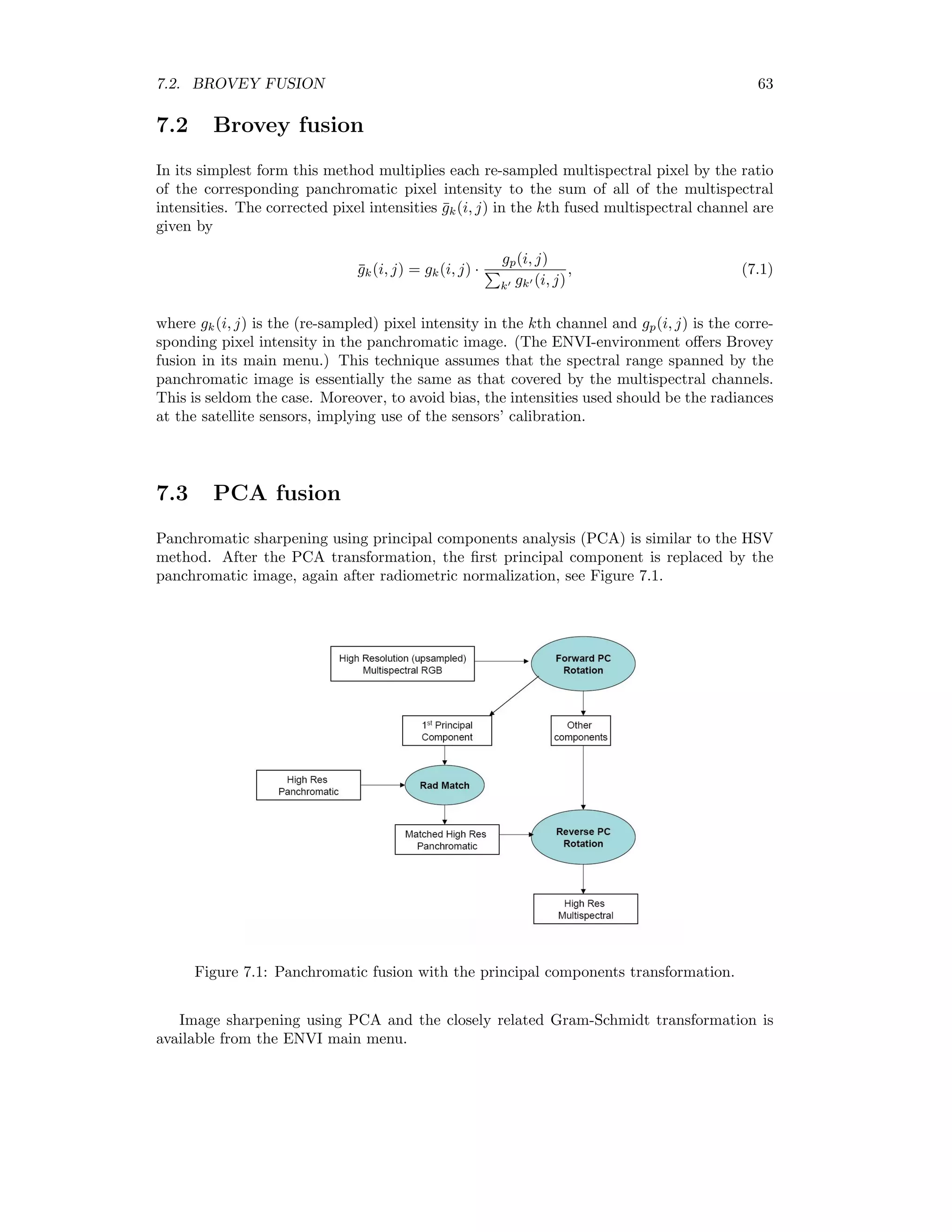
![62 CHAPTER 7. IMAGE SHARPENING axis of the RGB color cube. The coordinates in the new reference system are given by m1 m2 i1 = 2/ √ 6 −1/ √ 6 −1/ √ 6 0 1/ √ 2 −1/ √ 2 1/ √ 3 1/ √ 3 1/ √ 3 · R G B . Then the the rectangular coordinates (m1, m2, i1) are transformed into the cylindrical HSV coordinates: H = arctan(m1/m2), S = m2 1 + m2 2, I = √ 3 i1. The following IDL code illustrates the necessary steps for HSV fusion making use of ENVI batch procedures. These are also invoked directly from the ENVI main menu. pro HSVFusion, event ; get MS image envi_select, title=’Select low resolution three-band input file’, $ fid=fid1, dims=dims1, pos=pos1 if (fid1 eq -1) or (n_elements(pos1) ne 3) then return ; get PAN image envi_select, title=’Select panchromatic image’, $ fid=fid2, pos=pos2, dims=dims2, /band_only if (fid2 eq -1) then return envi_check_save, /transform ; linear stretch the images and convert to byte format envi_doit,’stretch_doit’, fid=fid1, dims=dims1, pos=pos1, method=1, $ r_fid=r_fid1, out_min=0, out_max=255, $ range_by=0, i_min=0, i_max=100, out_dt=1, out_name=’c:temphsv_temp’ envi_doit,’stretch_doit’, fid=fid2, dims=dims2, pos=pos2, method=1, $ r_fid=r_fid2, out_min=0, out_max=255, $ range_by=0, i_min=0, i_max=100, out_dt=1, /in_memory envi_file_query, r_fid2, ns=f_ns, nl=f_nl f_dims = [-1l, 0, f_ns-1, 0, f_nl-1] ; HSV sharpening envi_doit, ’sharpen_doit’, $ fid=[r_fid1,r_fid1,r_fid1], pos=[0,1,2], f_fid=r_fid2, $ f_dims=f_dims, f_pos=[0], method=0, interp=0, /in_memory ; remove temporary files from ENVI envi_file_mng, id=r_fid1, /remove, /delete envi_file_mng, id=r_fid2, /remove end](https://image.slidesharecdn.com/mortonjohncanty-imageanalysisandpatternrecognitionforremotesensingwithalgorithmsinenvi-idl-190425063306/75/Morton-john-canty-image-analysis-and-pattern-recognition-for-remote-sensing-with-algorithms-in-envi-idl-70-2048.jpg)
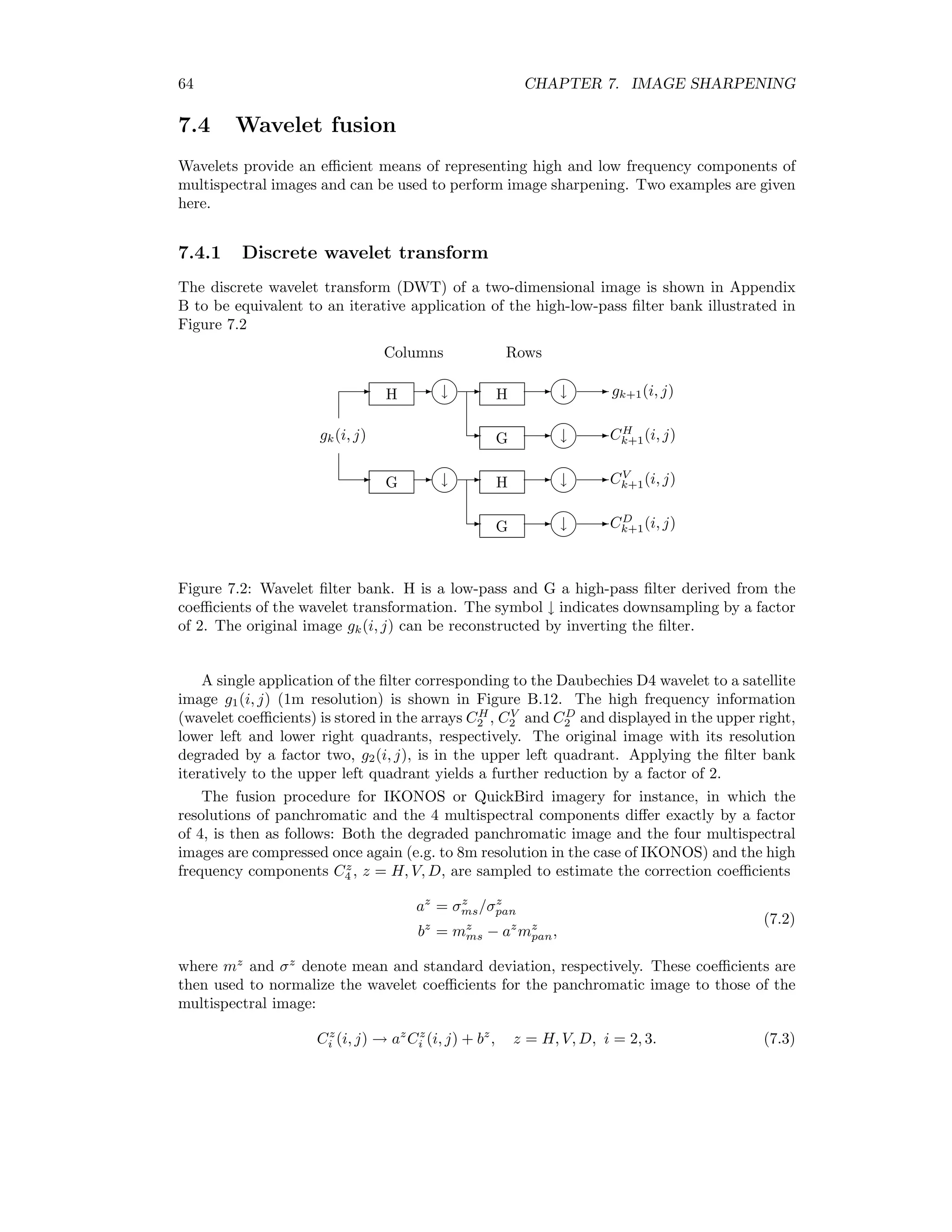
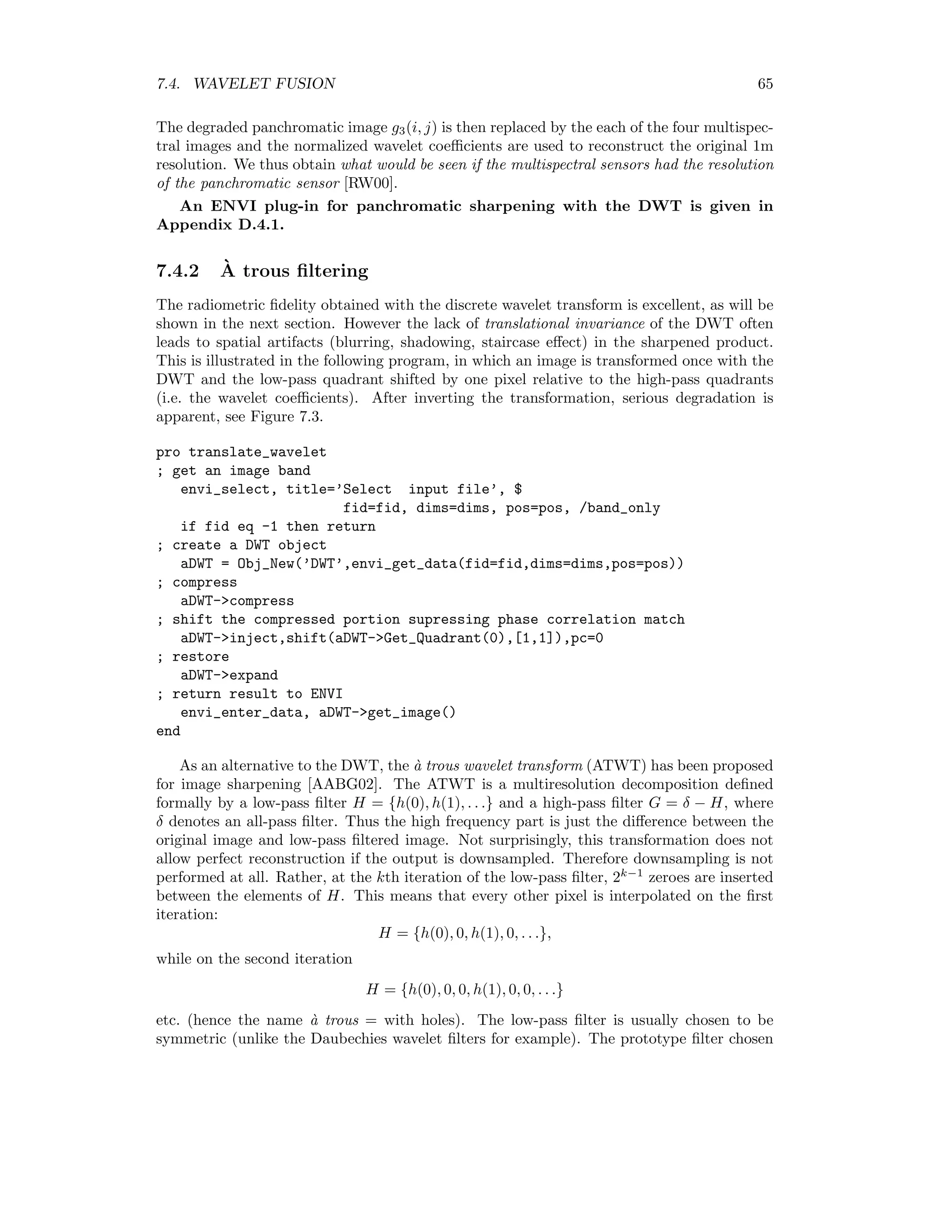
![7.4. WAVELET FUSION 65 The degraded panchromatic image g3(i, j) is then replaced by the each of the four multispec- tral images and the normalized wavelet coefficients are used to reconstruct the original 1m resolution. We thus obtain what would be seen if the multispectral sensors had the resolution of the panchromatic sensor [RW00]. An ENVI plug-in for panchromatic sharpening with the DWT is given in Appendix D.4.1. 7.4.2 `A trous filtering The radiometric fidelity obtained with the discrete wavelet transform is excellent, as will be shown in the next section. However the lack of translational invariance of the DWT often leads to spatial artifacts (blurring, shadowing, staircase effect) in the sharpened product. This is illustrated in the following program, in which an image is transformed once with the DWT and the low-pass quadrant shifted by one pixel relative to the high-pass quadrants (i.e. the wavelet coefficients). After inverting the transformation, serious degradation is apparent, see Figure 7.3. pro translate_wavelet ; get an image band envi_select, title=’Select input file’, $ fid=fid, dims=dims, pos=pos, /band_only if fid eq -1 then return ; create a DWT object aDWT = Obj_New(’DWT’,envi_get_data(fid=fid,dims=dims,pos=pos)) ; compress aDWT-compress ; shift the compressed portion supressing phase correlation match aDWT-inject,shift(aDWT-Get_Quadrant(0),[1,1]),pc=0 ; restore aDWT-expand ; return result to ENVI envi_enter_data, aDWT-get_image() end As an alternative to the DWT, the `a trous wavelet transform (ATWT) has been proposed for image sharpening [AABG02]. The ATWT is a multiresolution decomposition defined formally by a low-pass filter H = {h(0), h(1), . . .} and a high-pass filter G = δ − H, where δ denotes an all-pass filter. Thus the high frequency part is just the difference between the original image and low-pass filtered image. Not surprisingly, this transformation does not allow perfect reconstruction if the output is downsampled. Therefore downsampling is not performed at all. Rather, at the kth iteration of the low-pass filter, 2k−1 zeroes are inserted between the elements of H. This means that every other pixel is interpolated on the first iteration: H = {h(0), 0, h(1), 0, . . .}, while on the second iteration H = {h(0), 0, 0, h(1), 0, 0, . . .} etc. (hence the name `a trous = with holes). The low-pass filter is usually chosen to be symmetric (unlike the Daubechies wavelet filters for example). The prototype filter chosen](https://image.slidesharecdn.com/mortonjohncanty-imageanalysisandpatternrecognitionforremotesensingwithalgorithmsinenvi-idl-190425063306/75/Morton-john-canty-image-analysis-and-pattern-recognition-for-remote-sensing-with-algorithms-in-envi-idl-79-2048.jpg)
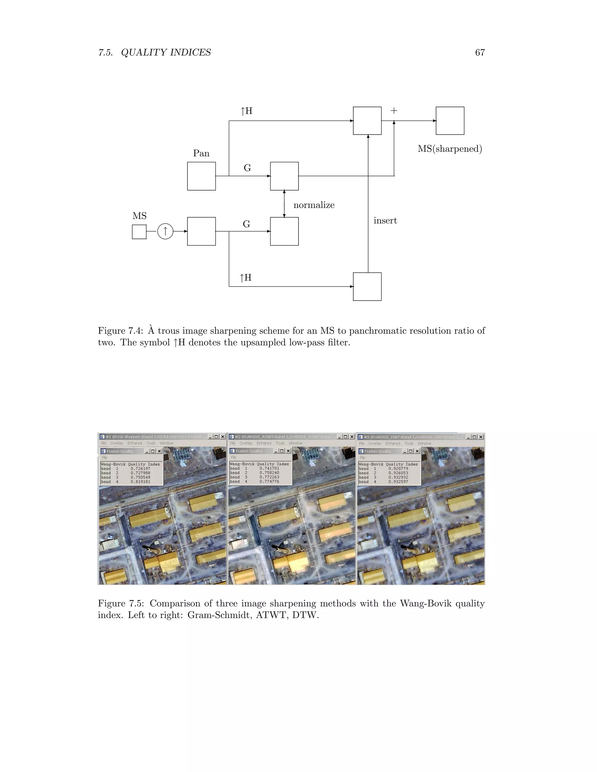
![66 CHAPTER 7. IMAGE SHARPENING here is the cubic B-spline filter H = {1/16, 1/4, 3/8, 1/4, 1/16}. The transformation is highly redundant and requires considerably more computer storage to implement. However when used for image sharpening it is much less sensitive to mis- alignment between the multispectral and panchromatic images. Figure 7.3: Artifacts due to lack of translational invariance of the DWT. Figure 7.4 outlines the scheme implemented in the ENVI plug-in for ATWT panchromatic sharpening. The MS band is nearest-neighbor upsampled by a factor of 2 to match the dimensions of the high resolution band. The `a trous transformation is applied to both bands (columns and rows are filtered with the upsampled cubic spline filter, with the difference determining the high-pass result). The high frequency component of the pan image is normalized to that of the MS image in the same way as for DWT sharpening, equations (7.2) and (7.3). Then the low frequency pan component is replaced by the filtered MS image and the transformation inverted. An ENVI plug-in for ATWT sharpening is described in Appendix D.4.2. 7.5 Quality indices Wang and Bovik [WB02] suggest the following measure of radiometric fidelity between two image bands f and g:](https://image.slidesharecdn.com/mortonjohncanty-imageanalysisandpatternrecognitionforremotesensingwithalgorithmsinenvi-idl-190425063306/75/Morton-john-canty-image-analysis-and-pattern-recognition-for-remote-sensing-with-algorithms-in-envi-idl-80-2048.jpg)
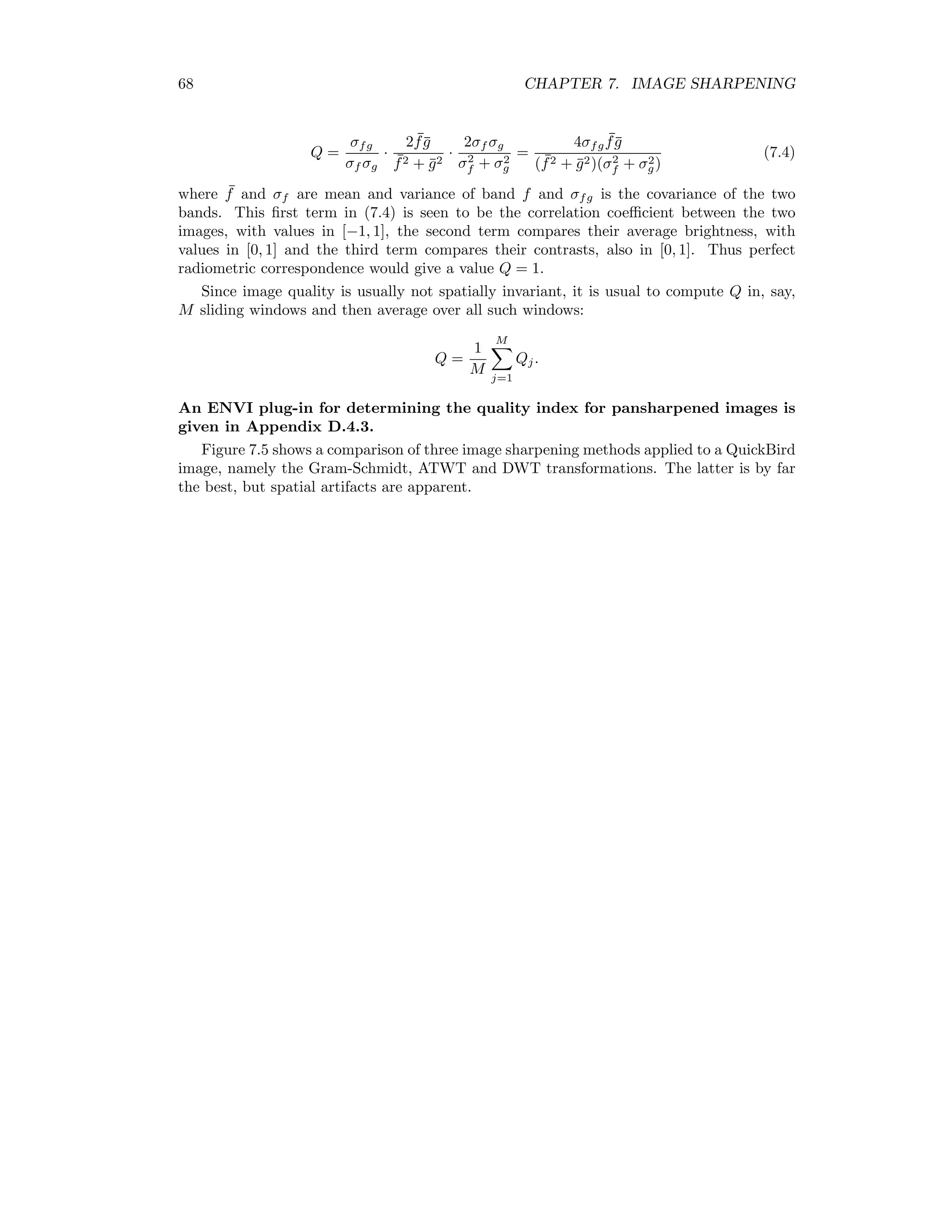
![68 CHAPTER 7. IMAGE SHARPENING Q = σfg σf σg · 2 ¯f¯g ¯f2 + ¯g2 · 2σf σg σ2 f + σ2 g = 4σfg ¯f¯g ( ¯f2 + ¯g2)(σ2 f + σ2 g) (7.4) where ¯f and σf are mean and variance of band f and σfg is the covariance of the two bands. This first term in (7.4) is seen to be the correlation coefficient between the two images, with values in [−1, 1], the second term compares their average brightness, with values in [0, 1] and the third term compares their contrasts, also in [0, 1]. Thus perfect radiometric correspondence would give a value Q = 1. Since image quality is usually not spatially invariant, it is usual to compute Q in, say, M sliding windows and then average over all such windows: Q = 1 M M j=1 Qj. An ENVI plug-in for determining the quality index for pansharpened images is given in Appendix D.4.3. Figure 7.5 shows a comparison of three image sharpening methods applied to a QuickBird image, namely the Gram-Schmidt, ATWT and DWT transformations. The latter is by far the best, but spatial artifacts are apparent.](https://image.slidesharecdn.com/mortonjohncanty-imageanalysisandpatternrecognitionforremotesensingwithalgorithmsinenvi-idl-190425063306/75/Morton-john-canty-image-analysis-and-pattern-recognition-for-remote-sensing-with-algorithms-in-envi-idl-83-2048.jpg)
![Chapter 8 Change Detection To quote Singh’s review article on change detection [Sin89], “The basic premise in using remote sensing data for change detection is that changes in land cover must result in changes in radiance values ... [which] must be large with respect to radiance changes from other factors.” In the present chapter we will mention briefly the most commonly used digital techniques for enhancing this “change signal” in bitemporal satellite images, and then focus our attention on the so-called multivariate alteration detection algorithm of Nielsen et al. [NCS98]. 8.1 Algebraic methods In order to see changes in the two multispectral images represented by N-dimensional ran- dom vectors F and G, a simple procedure is to subtract them from each other component- by-component, examining the N differenced images characterized by F − G = (F1 − G1, F2 − G2 . . . FN − GN ) (8.1) for significant changes. Pixel intensity differences near zero indicate no change, large positive or negative values indicate change, and decision thresholds can be set to define significant changes. If the difference signatures in the spectral channels are used to classify the kind of change that has taken place, one speaks of change vector analysis. Thresholds are usually expressed in standard deviations from the mean difference value, which is taken to correspond to no change. Alternatively, ratios of intensities of the form Fk Gk , k = 1 . . . N (8.2) can be built between successive images. Ratios near unity correspond to no-change, while small and large values indicate change. A disadvantage of this method is that random variables of the form (8.2) are not normally distributed, so simple threshold values defined in terms of standard deviations are not valid. Other algebraic combinations, such as differences in vegetation indices (Section 2.1) are also in use. All of these “band math” operations can of course be performed conveniently within the ENVI/IDL environment. 69](https://image.slidesharecdn.com/mortonjohncanty-imageanalysisandpatternrecognitionforremotesensingwithalgorithmsinenvi-idl-190425063306/75/Morton-john-canty-image-analysis-and-pattern-recognition-for-remote-sensing-with-algorithms-in-envi-idl-84-2048.jpg)
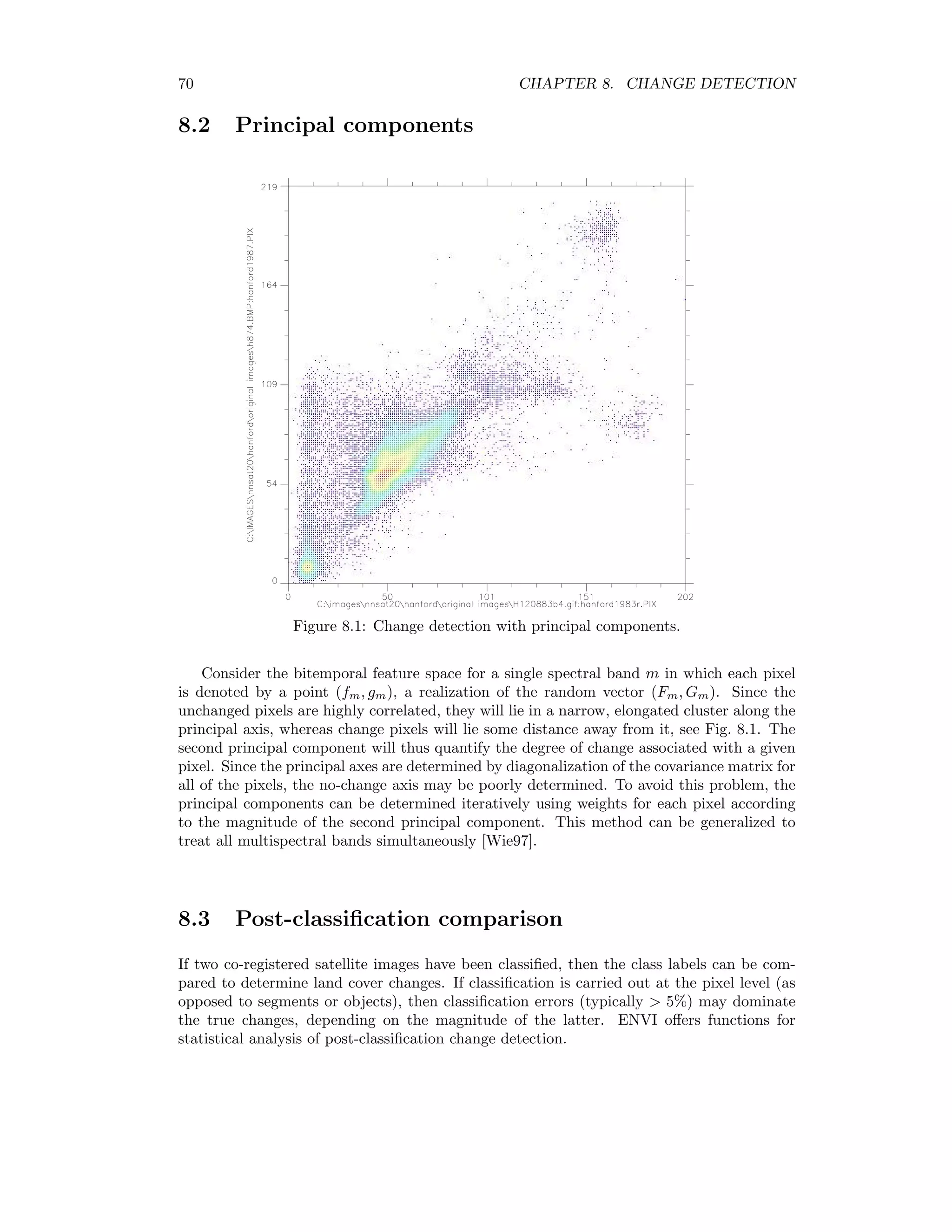
![70 CHAPTER 8. CHANGE DETECTION 8.2 Principal components Figure 8.1: Change detection with principal components. Consider the bitemporal feature space for a single spectral band m in which each pixel is denoted by a point (fm, gm), a realization of the random vector (Fm, Gm). Since the unchanged pixels are highly correlated, they will lie in a narrow, elongated cluster along the principal axis, whereas change pixels will lie some distance away from it, see Fig. 8.1. The second principal component will thus quantify the degree of change associated with a given pixel. Since the principal axes are determined by diagonalization of the covariance matrix for all of the pixels, the no-change axis may be poorly determined. To avoid this problem, the principal components can be determined iteratively using weights for each pixel according to the magnitude of the second principal component. This method can be generalized to treat all multispectral bands simultaneously [Wie97]. 8.3 Post-classification comparison If two co-registered satellite images have been classified, then the class labels can be com- pared to determine land cover changes. If classification is carried out at the pixel level (as opposed to segments or objects), then classification errors (typically 5%) may dominate the true changes, depending on the magnitude of the latter. ENVI offers functions for statistical analysis of post-classification change detection.](https://image.slidesharecdn.com/mortonjohncanty-imageanalysisandpatternrecognitionforremotesensingwithalgorithmsinenvi-idl-190425063306/75/Morton-john-canty-image-analysis-and-pattern-recognition-for-remote-sensing-with-algorithms-in-envi-idl-85-2048.jpg)
![8.4. MULTIVARIATE ALTERATION DETECTION 71 8.4 Multivariate alteration detection Suppose we make a linear combination of the intensities for all N channels in the first image acquired at time t2, represented by the random vector F. That is, we create a single image whose pixel intensities are U = a F = a1F1 + a2F2 + . . . aN FN , where the vector of coefficients a is as yet unspecified. We do the same for t2, i.e. we make the linear combination V = b G, and then look at the scalar difference image U − V . This procedure combines all the information into a single image, whereby one still hast to choose the coefficients a and b in some suitable way. Nielsen et al. [NCS98] suggest determining the coefficients so that the positive correlation between U and V is minimized. This means that the resulting difference image U − V will show maximum spread in its pixel intensities. If we assume that the spread is primarily due to actual changes that have taken place in the scene over the interval t2 − t1, then this procedure will enhance those changes as much as possible. Specifically we seek linear combinations such that var(U − V ) = var(U) + var(V ) − 2cov(U, V ) → maximum, (8.3) subject to the constraints var(U) = var(V ) = 1. (8.4) Note that under these constraints var(U − V ) = 2(1 − ρ), (8.5) where ρ is the correlation of the transformed vectors U and V , ρ = corr(U, V ) = cov(U, V ) var(U)var(V ) . Since we are dealing with change detection, we require that the random variables U and V be positively correlated, that is, cov(U, V ) 0. We thus seek vectors a and b which minimize the positive correlation ρ. 8.4.1 Canonical correlation analysis Canonical correlation analysis leads to a transformation of each set of variables F and G such that their mutual correlation is displayed unambiguously, see [And84], Chapter 12. We can derive the transformation as follows: For multivariate normally distributed data the combined random vector is distributed as F G ∼ N 0 0 , Σff Σfg Σgf Σgg . Recalling the property (1.6) we have var(U) = a Σff a, var(V ) = b Σggb, cov(U, V ) = a Σfgb.](https://image.slidesharecdn.com/mortonjohncanty-imageanalysisandpatternrecognitionforremotesensingwithalgorithmsinenvi-idl-190425063306/75/Morton-john-canty-image-analysis-and-pattern-recognition-for-remote-sensing-with-algorithms-in-envi-idl-86-2048.jpg)
![72 CHAPTER 8. CHANGE DETECTION If we introduce the Lagrange multipliers ν/2 and µ/2, extremalizing the covariance cov(U, V ) under the constraints (8.4) is equivalent to extremalizing the unconstrained Lagrange func- tion L = a Σfgb − ν 2 (a Σff a − 1) − µ 2 (b Σggb − 1). Differentiating, we obtain ∂L ∂a = Σfgb − ν 2 2Σff a = 0, ∂L ∂b = Σfga − µ 2 2Σggb = 0 or a = 1 ν Σ−1 ff Σfgb, b = 1 µ Σ−1 gg Σfga. The correlation between the random variables U and V is ρ = cov(U, V ) var(U)var(V ) = a Σfgb a Σff a b Σggb . Substituting for a and b in this equation gives (with Σfg = Σgf ) ρ2 = a ΣfgΣ−1 gg Σgf a a Σff a , ρ2 = b Σgf Σ−1 ff Σfgb b Σggb , which are equivalent to the two generalized eigenvalue problems ΣfgΣ−1 gg Σgf a = ρ2 Σff a Σgf Σ−1 ff Σfgb = ρ2 Σggb. (8.6) Thus the desired projections U = a F are given by the eigenvectors a1 . . . aN corresponding to the generalized eigenvalues ρ2 ∼ λ1 ≥ . . . ≥ λN of ΣfgΣ−1 gg Σgf with respect to Σff . Similarly the desired projections V = b G are given by the eigenvectors b1 . . . bN of Σgf Σ−1 ff Σfg with respect to Σgg corresponding to the same eigenvalues. Nielsen et al. [NCS98] refer to the N difference components Mi = Ui − Vi = ai F − bi G, i = 1 . . . N, (8.7) as the multivariate alteration detection (MAD) components of the combined bitemporal image. 8.4.2 Solution by Cholesky factorization Equations (8.6) are of the form Σ1a = λΣa, where both Σ1 and Σ are symmetric and Σ is positive definite. The Cholesky factorization of Σ is Σ = LL , where L is a lower triangular matrix, and can be thought of as the “square root” of Σ. Such an L always exists is Σ is positive definite. Therefore we can write Σ1a = LL a](https://image.slidesharecdn.com/mortonjohncanty-imageanalysisandpatternrecognitionforremotesensingwithalgorithmsinenvi-idl-190425063306/75/Morton-john-canty-image-analysis-and-pattern-recognition-for-remote-sensing-with-algorithms-in-envi-idl-87-2048.jpg)
![8.4. MULTIVARIATE ALTERATION DETECTION 73 or, equivalently, L−1 Σ1(L )−1 L a = λL a or, with d = L a and commutivity of inverse and transpose, [L−1 Σ1(L−1 ) ]d = λd, a standard eigenproblem for a real, symmetric matrix L−1 Σ1(L−1 ) . Let the (orthogonal) eigenvectors be di. We have 0 = di dj = ai LL aj = ai Σaj, i = j. (8.8) 8.4.3 Properties of the MAD components We have, from (8.4) and (8.8), for the eigenvectors ai and bi, ai Σff aj = bi Σggbj = δij. Furthermore bi = 1 √ λi Σ−1 gg Σgf ai, i.e. substituting this into the LHS of the second equation in (8.6): Σgf Σ−1 ff Σfg 1 √ λi Σ−1 gg Σgf ai = Σgf Σ−1 ff 1 √ λi λiΣff ai = Σgf λiai = λiΣggbi, as required. It follows that ai Σfgbj = ai 1 λj ΣfgΣ−1 gg Σgf aj = λj ai Σff ai = λj δij, and similarly for bi Σgf aj. Thus the covariances of the MAD components are given by cov(Ui − Vi, Uj − Vj) = cov(ai F − bi G, aj F − bj G) = 2δij(1 − λj). The MAD components are therefore orthogonal (uncorrelated) with variances var(Ui − Vi) = σ2 MADi = 2(1 − λi). (8.9) The transformation corresponding to the smallest eigenvalue, namely (aN , bN ), will thus give maximal variance for the difference U − V . We can derive change probabilities from a MAD image as follows. The sum of the squares of the standardized MAD components for no-change pixels, given by Z = MAD1 σMAD1 2 + . . . + MADN σMADN 2 , is approximately chi-square distributed with N degrees of freedom, i.e., Pr(Z ≤ z) = ΓP (N/2, z/2). For a given measured value z for some pixel, the probability that Z could be that large or larger, given that the pixel is no-change, is 1 − ΓP (N/2, z/2).](https://image.slidesharecdn.com/mortonjohncanty-imageanalysisandpatternrecognitionforremotesensingwithalgorithmsinenvi-idl-190425063306/75/Morton-john-canty-image-analysis-and-pattern-recognition-for-remote-sensing-with-algorithms-in-envi-idl-88-2048.jpg)
![8.4. MULTIVARIATE ALTERATION DETECTION 75 which are identical to (8.6) with b = T c. Therefore the MAD components in the trans- formed situation are ai F − ci H = ai F − ci TG = ai F − (T ci) G = ai F − bi G as before. 8.4.6 Improving signal to noise The MAD transformation can be augmented by subsequent application of the maximum autocorrelation factor (MAF) transformation, in order to improve the spatial coherence of the difference components, see [NCS98]. When image noise is estimated as the difference between intensities of neighboring pixels, the MAF transformation is equivalent to the MNF transformation. The MAF/MAD variates thus generated are also orthogonal and invariant under affine transformations. An ENVI plug-in for performing the MAF transfor- mation is given in Appendix D.5.2. 8.4.7 Decision thresholds Since the MAD components are approximately normally distributed about zero and uncor- related, see Figure 8.2, decision thresholds for change or no change pixels can be set in terms of standard deviations about the mean for each component separately. This can be done arbitrarily, for example by saying that all pixels in a MAD component whose intensities are within ±2σMAD are no-change pixels. Figure 8.2: Scatter plot of two MAD components. We can do better than this, however, using a Bayesean technique. Let us consider the following mixture model for a random variable X representing one of the MAD components: p(x) = p(x | NC)p(NC) + p(x | C−)p(C−) + p(x | C+)p(C+), (8.11)](https://image.slidesharecdn.com/mortonjohncanty-imageanalysisandpatternrecognitionforremotesensingwithalgorithmsinenvi-idl-190425063306/75/Morton-john-canty-image-analysis-and-pattern-recognition-for-remote-sensing-with-algorithms-in-envi-idl-90-2048.jpg)
![76 CHAPTER 8. CHANGE DETECTION Figure 8.3: Probability mixture model for MAD components. where C+, C− and NC denote positive change, negative change and no change, respectively, see Fig. 8.3. The set of measurements S = {xi} may be grouped into four disjoint sets: SNC, SC−, SC+, SU = SSNC ∪ SC− ∪ SC+, with SU denoting the set of ambiguous pixels.1 From the sample mean and sample variance, we estimate initially the moments for the distribution of no-change pixels: µNC = 1 |SNC| · i∈SNC xi, (σNC)2 = 1 |SNC| · i∈SNC (xi − µNC)2 (|S| denotes set cardinality) and similarly for C− and C+. Bruzzone and Prieto [BP00] suggest improving these estimates by using the pixels in SU and applying the so-called EM algorithm (see [Bis95] for a good explanation): µNC = i∈S p(NC | xi)xi / i∈S p(NC | xi) (σNC)2 = i∈S p(NC | xi)(xi − µNC)2 / i∈S p(NC | xi) p (NC) = 1 |S| · i∈S p(NC | xi) , (8.12) where p(NC | xi) is the a posteriori probability for a no-change pixel conditional on mea- surement xi. We have the following rules for determining p(NC | xi): 1. i ∈ SNC : p(NC | xi) = 1 2. i ∈ SC± : p(NC | xi) = 0 1The symbols ∪ and denote set union and set difference, respectively. These sets can be determined in practice by setting generous, scene-independent thresholds for change and no-change pixel intensities, see [BP00].](https://image.slidesharecdn.com/mortonjohncanty-imageanalysisandpatternrecognitionforremotesensingwithalgorithmsinenvi-idl-190425063306/75/Morton-john-canty-image-analysis-and-pattern-recognition-for-remote-sensing-with-algorithms-in-envi-idl-91-2048.jpg)
![78 CHAPTER 8. CHANGE DETECTION homogeneous and can be approximated by linear functions. The critical aspect is the deter- mination of suitable time-invariant features upon which to base the normalization. As we have seen, the MAD transformation invariant to linear and affine scaling. Thus, if one uses MAD for change detection applications, preprocessing by linear radiometric normal- ization is superfluous. However radiometric normalization of imagery is important for many other applications, such as mosaicing, tracking vegetation indices over time, supervised and unsupervised land cover classification, etc. Furthermore, if some other, non-invariant change detection procedure is preferred, it must generally be preceded by radiometric normaliza- tion [CNS04]. Taking advantage of this invariance, one can apply the MAD transformation to select the no-change pixels in bitemporal images, and then used them for radiometric normalization. The procedure is simple, fast and completely automatic and compares very favorably with normalization using hand-selected, time-invariant features. An ENVI plug-in for radiometric normalization with the MAD transforma- tion is given in Appendix D.5.3.](https://image.slidesharecdn.com/mortonjohncanty-imageanalysisandpatternrecognitionforremotesensingwithalgorithmsinenvi-idl-190425063306/75/Morton-john-canty-image-analysis-and-pattern-recognition-for-remote-sensing-with-algorithms-in-envi-idl-93-2048.jpg)
![80 CHAPTER 9. UNSUPERVISED CLASSIFICATION clustering given the data. From Bayes’ rule, p(C | x) = p(x | C)p(C) p(x) . (9.2) The quantity p(x|C) is the joint probability density function for clustering C, also referred to as the likelihood of observing the clustering C given the data x, P(C) is the prior probability for C and p(x) is a normalization independent of C. The joint probability density for the data is the product of the individual probability densities, i.e., p(x | C) = K k=1 i∈Ck p(xi | Ck) = K k=1 i∈Ck (2π)−N/2 |Σk|−1/2 exp − 1 2 (xi − µk) Σ−1 k (xi − µk) . Forming the product in this way is justified by the independence of the samples. The log-likelihood is given by [Fra96] L = log p(x | C) = K k=1 i∈Ck − N 2 log(2π) − 1 2 log |Σk| − 1 2 (xi − µk) Σ−1 k (xi − µk) . With (9.2) we can therefore write log p(C | x) ∝ L + log p(C). (9.3) If all K classes exhibit identical covariance matrices according to Σk = σ2 I, k = 1 . . . K, (9.4) where I is the identity matrix, then L is maximized when the expression K k=1 i∈Ck (xi) − µk) ( 1 2σ2 I)(xi − µk) = K k=1 i∈Ck (xi − µk) (xi − µk) 2σ2 is minimized. We are thus led to the cost function E(C) = K k=1 i∈Ck (xi − µk) (xi − µk) 2σ2 − log p(C). (9.5) An optimal clustering C under these assumptions is achieved for E(C) → min . Now we introduce a “hard” class dependency in the form of a matrix u with elements given by uki = 1 if i ∈ Ck 0 otherwise. (9.6)](https://image.slidesharecdn.com/mortonjohncanty-imageanalysisandpatternrecognitionforremotesensingwithalgorithmsinenvi-idl-190425063306/75/Morton-john-canty-image-analysis-and-pattern-recognition-for-remote-sensing-with-algorithms-in-envi-idl-95-2048.jpg)
![9.2. ALGORITHMS THAT MINIMIZE THE SIMPLE COST FUNCTION 81 The matrix u satisfies the conditions K k=1 uki = 1, i = 1 . . . n, (9.7) meaning that each sampled pixel xi, i = 1 . . . n, belongs to precisely one class, and n i=1 uki 0, k = 1 . . . K, (9.8) meaning that no class Ck, k = 1 . . . K, is empty. The sum in (9.8) is the number nk of pixels in the kth class. An unbiased estimate mk of the expected value µk for the kth cluster is therefore given by µk ≈ mk = 1 nk i∈Ck xi = n i=1 ukixi n i=1 uki , k = 1 . . . K, (9.9) and an estimate Fk of the covariance matrix Σk by Σk ≈ Fk = n i=1 uki(xi − mk)(xi − mk) n i=1 uki , k = 1 . . . K. (9.10) We can now write (9.5) in the form E(C) = K k=1 n i=1 uki (xi − mk) (xi − mk) 2σ2 − log p(C). (9.11) Finally, if we do not wish to include prior probabilities, we can simply say that all clustering configurations C are a priori equally likely. Then the last term in (refe911) is independent of C and we have, dropping the multiplicative constant 1/2σ2 , the well-known sum-of-squares cost function E(C) = K k=1 n i=1 uki(xi − mk) (xi − mk). (9.12) 9.2 Algorithms that minimize the simple cost function We begin with the popular K-means method and then consider an algorithm due to (Palu- binskas 1998) [Pal98], which uses cost function (9.11) and for which the number of clusters is determined automatically. Then we discuss a common version of bottom-up or agglomer- ative hierarchical clustering, and finally a “fuzzy” version of the K-means algorithm. 9.2.1 K-means The K-means clustering algorithm (KM) (sometimes referred to as basic Isodata [DH73] or migrating means [JRR99]) is based on the cost function (9.12). After initialization of the cluster centers, the distance measure corresponding to a minimization of (9.12), namely d(i, k) = (xi − mk) (xi − mk) is used to re-cluster the pixel vectors. Then (9.9) is used to recalculate the cluster centers. This procedure is iterated until the centers cease to change significantly. K-means clustering may be performed within the ENVI environment from the main menu.](https://image.slidesharecdn.com/mortonjohncanty-imageanalysisandpatternrecognitionforremotesensingwithalgorithmsinenvi-idl-190425063306/75/Morton-john-canty-image-analysis-and-pattern-recognition-for-remote-sensing-with-algorithms-in-envi-idl-96-2048.jpg)
![82 CHAPTER 9. UNSUPERVISED CLASSIFICATION 9.2.2 Extended K-means Denote by pk = p(Ck) the prior probability for cluster k. The entropy S associated with this prior distribution is S = − K k=1 pk log pk. (9.13) Distributions with high entropy are those for which the pi are all similar, that is, the pixels are distributed evenly over all available clusters, see [Bis95]. Low entropy means that most of the data are concentrated in very few clusters. We choose a prior distribution p(C) in (9.11) for which few clusters are more probable than many clusters, namely p(C) ∝ exp(−αES) = exp αE K k=1 pk log pk , where αE is a parameter. The cost function (9.11) can then be written as E(C) = K k=1 n i=1 uki (xi − mk) (xi − mk) 2σ2 − αE K k=1 pk log pk. (9.14) With pk ≈ nk n = 1 n n i=1 uki (9.15) this becomes E(C) = K k=1 n i=1 uki (xi − mk) (xi − mk) 2σ2 − αE n log pk . (9.16) An estimate for the parameter αE may be obtained as follows [Pal98]: From (9.14) and (9.15) E(C) ≈ K k=1 nσ2 kpk 2σ2 − αEpk log pk . Equating the likelihood and prior terms in this expression and taking σ2 k ≈ σ2 and pk ≈ 1/ ˜K, where ˜K is some a priori expected number of clusters, gives αE ≈ − n 2 log(1/ ˜K) . (9.17) The parameter σ2 can be estimated from the data. The extended K-means (EKM) algorithm is as follows: First an initial configuration with a very large number of clusters K is chosen (for one-dimensional data this might conveniently be the 256 gray values that a pixel with 8-bit resolution can have) and initial values mk = 1 nk n i=1 ukixi, pk = nk n (9.18) are determined. Then the data are re-clustered according to the distance measure corre- sponding to a minimization of (9.16): d(i, k) = (xi − mk) (xi − mk) 2σ2 − αE n log pk. (9.19)](https://image.slidesharecdn.com/mortonjohncanty-imageanalysisandpatternrecognitionforremotesensingwithalgorithmsinenvi-idl-190425063306/75/Morton-john-canty-image-analysis-and-pattern-recognition-for-remote-sensing-with-algorithms-in-envi-idl-97-2048.jpg)
![9.2. ALGORITHMS THAT MINIMIZE THE SIMPLE COST FUNCTION 83 The prior term tends to reduce the number of clusters and any class which has in the course of the algorithm nk = 0 is simply dropped from the calculation. (Condition (9.8) is thus relaxed.) Iteration of (9.18) and (9.19) continues until no significant changes in the mk occur. The explicit choice of the number of clusters K is replaced by the necessity of choosing a value for the “meta-parameter” αE. This has the advantage that we can use one parameter for a wide variety of images and let the algorithm itself decide on the actual value of K in any given instance. 9.2.3 Agglomerative hierarchical clustering The agglomerative hierarchical clustering algorithm that we consider here is, as for K-means, based on the cost function (9.12), see [DH73]. It begins by assigning each pixel in the dataset to its own class or cluster. At this stage of course, the cost function E(C), Eq. (9.12), is zero. We write E(C) in the form E(C) = K k=1 Ek (9.20) where Ek is given by Ek = i∈Ck (xi − mk) (xi − mk). Every agglomeration of clusters to form a smaller number of clusters will increase E(C). We therefore seek a prescription for choosing two clusters for combination that will increase E(C) by the smallest amount possible. Suppose clusters k with nk members and with n members are merged, k , and the new cluster is labeled k. Then mk → nkmk + n m nk + n =: ¯m. Thus after the agglomeration, Ek changes to Ek = i∈Ck∪C (xi − ¯m) (xi − ¯m) and E disappears. The net change in E(C) is therefore, after some algebra, ∆(k, ) = i∈Ck∪C (xi − ¯m) (xi − ¯m) − i∈Ck (xi − mk) (xi − mk) − i∈C (xi − m ) (xi − m ) = nkn nk + n (mk − m ) (mk − m ). (9.21) The minimum increase in E(C) is achieved by combining those two clusters k and which minimize the above expression. Given two alternative candidate cluster pairs with simi- lar combined memberships nk + n and whose means have similar euclidean separations mk − m , this prescription obviously favors combining that pair with the larger discrep- ancy between nk and n . Thus similar-sized clusters are preserved and smaller clusters are absorbed by larger ones.](https://image.slidesharecdn.com/mortonjohncanty-imageanalysisandpatternrecognitionforremotesensingwithalgorithmsinenvi-idl-190425063306/75/Morton-john-canty-image-analysis-and-pattern-recognition-for-remote-sensing-with-algorithms-in-envi-idl-98-2048.jpg)
![84 CHAPTER 9. UNSUPERVISED CLASSIFICATION Let k, represent the cluster formed by combination of the clusters k and . Then the increase in cost incurred by combining this cluster with cluster r can be determined from (9.21) as ∆( k, , r) = (nk + nr)∆(k, r) + (n + nr)∆( , r) − nr∆(k, ) nk + n + nr . (9.22) Once ∆(i, j) = 1 2 (xi − xj) (xi − xj) for i, j = 1 . . . n has been initialized from (9.21) for all possible combinations of pixels, the recursive formula (9.22) can be used to calculate efficiently the cost function for any further combinations without reference to the original data. The algorithm terminates when the desired number of clusters has been reached or continues until a single cluster has been formed. Assuming that the data consist of ˜K compact and well separated clusters, the slope of E(C) vs. the number of clusters K should decrease (become more negative) for K ≤ ˜K. An ENVI plug-in for agglomerative hierarchic clustering is given in Appendix D.6.1. 9.2.4 Fuzzy K-means For q 1 we write (9.9) and (9.12) in the equivalent forms [Dun73] mk = n i=1 uq kixi n i=1 uq ki , k = 1 . . . K, (9.23) E(C) = K k=1 n i=1 uq ki(xi − mk) (xi − mk), (9.24) and make the transition from “hard” to “fuzzy” clustering by replacing (9.6) by continuous variables 0 uki 1, k = 1 . . . K, i = 1 . . . n, (9.25) but retaining requirements (9.7) and (9.8). The matrix u is now a fuzzy class membership matrix. With i fixed, we seek values for the uki which solve the minimization problem Ei = K k=1 uq ki(xi − mk) (xi − mk) → min, i = 1 . . . n, under conditions (9.7). By introducing the Lagrange function Li = Ei − λ K k=1 uki − 1 we can equivalently solve the unconstrained problem Li → min. Differentiating with respect to uki, ∂Li ∂uki = q(uki)q−1 (xi − mk) (xi − mk) − λ = 0, k = 1 . . . K,](https://image.slidesharecdn.com/mortonjohncanty-imageanalysisandpatternrecognitionforremotesensingwithalgorithmsinenvi-idl-190425063306/75/Morton-john-canty-image-analysis-and-pattern-recognition-for-remote-sensing-with-algorithms-in-envi-idl-99-2048.jpg)
![9.3. EM CLUSTERING 85 from which we have uki = q−1 λ q q−1 1 (xi − mk) (xi − mk) . (9.26) The Lagrange multiplier λ is determined by 1 = K k=1 uki = q−1 λ q K k=1 q−1 1 (xi − mk) (xi − mk) , Substituting this into (9.26), we obtain finally uki = q−1 1 (xi−mk) (xi−mk) K k =1 q−1 1 (xi−mk ) (xi−mk ) , k = 1 . . . K, i = 1 . . . n. (9.27) The parameter q determines the “degree of fuzziness” and is usually chosen as q = 2. The fuzzy K-means (FKM) algorithm consists of a simple iteration of equations (9.23) and (9.27). The algorithm terminates when the cluster centers mk – or alternatively when the matrix elements uki – cease to change significantly. This algorithm should gives similar results to the K-means algorithm, but one expects it to be less likely to become trapped in local minima of the cost function. An ENVI plug-in for fuzzy k-means clustering is given in Appendix D.6.2. 9.3 EM Clustering The EM (= expectation maximization) algorithm, (see e.g. [Bis95]) replaces uki in (9.27) by the posterior probability p(Ck | xi) of class Ck given the observation xi. That is, using Bayes’ theorem, uki → p(Ck | xi) ∼ p(xi | Ck)p(Ck). Here p(xi | Ck) is taken to be a multivariate normal distribution function with estimated mean mk and estimated covariance matrix Fk given by (9.9) and (9.10), respectively. Thus uki ∼ p(Ck) 1 |Fk| exp − 1 2 (xi − mk) F−1 k (xi − mk) . (9.28) One can use the current class membership to estimate P(Ck) as pk according to (9.15). The EM algorithm is then an iteration of equations (9.9), (9.10), (9.15) and (9.28) with the same termination condition as for the fuzzy K-means algorithm, see also Eqs. (8.12). After each iteration the columns of u are normalized according to (9.7). Because of the exponential distance dependence of the membership probabilities in (9.28), the algorithm is very sensitive to initialization conditions, and can even become unstable. To avoid this problem, one can first obtain initial values for the mk and for u by preceding the calculation with the fuzzy K-means algorithm. Explicitly: Algorithm (EM clustering) 1. Determine starting values for cluster centers mk and initial memberships uki from the FKM algorithm.](https://image.slidesharecdn.com/mortonjohncanty-imageanalysisandpatternrecognitionforremotesensingwithalgorithmsinenvi-idl-190425063306/75/Morton-john-canty-image-analysis-and-pattern-recognition-for-remote-sensing-with-algorithms-in-envi-idl-100-2048.jpg)
![86 CHAPTER 9. UNSUPERVISED CLASSIFICATION 2. Determine the cluster centers mk with (9.9) and the prior probabilities P(Ck) with (9.15). 3. Calculate the weighted covariance matrices Fk with (9.10) and with (9.28) the class membership probabilities uki. Normalize the columns of u. 4. If u has not changed significantly, stop, else go to 2. 9.3.1 Simulated annealing Even with initialization using the fuzzy K-means algorithm the EM algorithm may be trapped in a local optimum. An alternative scheme is to apply so-called simulated annealing. Essentially the initial memberships are random and only gradually are the calculated class memberships allowed to influence the estimation of the class centers [Hil01]. The rate of reduction of randomness is determined by a temperature parameter. For example, the class memberships in (9.28) may replaced by uki → uki(1 − r1/T ) on each iteration, where T is initialized to T0 and reduced at each iteration by a factor c 1: T → cT and where r ∈ (0, 1) is a uniformly distributed random number. As T approaches zero, uki will be determined more and more by the probability distribution parameters alone in (9.28). 9.3.2 Partition density Since the simple cost function E(C) of (9.12) is no longer relevant, we choose with [GG89] the partition density as a criterion for choosing the best number of clusters. The fuzzy hypervolume, defined as FHV = K k=1 |Fk|, is proportional to the volume in feature space occupied by the ellipsoidal clusters generated by the algorithm. For instance, for a two dimensional cluster with an elliptical probability density we have, in its principal axis coordinate system, |Σ| = σ2 1 0 0 σ2 2 = σ1σ2 ≈ area (volume) of the ellipse. Summing the memberships of the observations within one standard deviation of each cluster center, S = n i=1 K k=1 uik, ∀i ∈ {i | (xi − mk) · F−1 k · (xi − mk) 1}, the partition density is defined as PD = S/FHV. (9.29) Assuming that the data consist of ˜K well-separated clusters of approximately multivari- ate normally distributed pixels, the partition density should exhibit a maximum at K = ˜K. An ENVI plug-in for EM clustering is given in Appendix D.6.3.](https://image.slidesharecdn.com/mortonjohncanty-imageanalysisandpatternrecognitionforremotesensingwithalgorithmsinenvi-idl-190425063306/75/Morton-john-canty-image-analysis-and-pattern-recognition-for-remote-sensing-with-algorithms-in-envi-idl-101-2048.jpg)
![9.3. EM CLUSTERING 87 9.3.3 Including spatial information The algorithms described thus far make exclusive use of the spectral properties of the in- dividual observations (pixels). Spatial relationships within an image such as large scale, coherent regions, textures etc. are ignored entirely. The EM algorithm determines the a posteriori class membership probabilities of each observation for the classes in question. In this section we describe a post-processing technique to take account of some of the spatial information implicit in the classified image in order to improve the original classification. This technique makes use of the vectors of a posteriori probabilities associated with each classified pixel. Figure 9.1 shows schematically a single pixel m together with its immediate neighborhood n, which we take to consist of the four pixels above, below, to the left and to the right of m. Let its a posteriori probabilities be Pm(Ck), k = 1 . . . M, M k=1 Pm(Ck) = 1, or, more simply, the vector Pm. 1 2 3 4 C Pixel mC Neighborhood n Figure 9.1: A pixel neighborhood. A possible misclassification of the pixel m could in principle be corrected by examining its neighborhood. The neighboring pixels would have in some way to modify Pm such that the maximal probability corresponds to the true class. We now describe a purely heuristic but nevertheless intuitively satisfying procedure to do just that, the so-called probabilistic label relaxation method [JRR99]. Let Qm(Ck) be a neighborhood function for the mth Pixel, which is supposed to correct Pm(Ck) in the above sense, according to the prescription Pm(Ck) = Pm(Ck)Qm(Ck) k Pm(Ck )Qm(Ck ) , k = 1 . . . M, or, as a vector equation, according to Pm = Pm ⊗ Qm PmQm , (9.30) where ⊗ signifies the Hadamard product, which simply means component-by-component multiplication. The denominator ensures that the result is also a probability, in other words](https://image.slidesharecdn.com/mortonjohncanty-imageanalysisandpatternrecognitionforremotesensingwithalgorithmsinenvi-idl-190425063306/75/Morton-john-canty-image-analysis-and-pattern-recognition-for-remote-sensing-with-algorithms-in-envi-idl-102-2048.jpg)
![9.4. THE KOHONEN SELF ORGANIZING MAP 89 2. Determine the average neighborhood vector Pn of all pixels m and replace Pm with Pm according to (9.32). Re-classify pixel m according to the largest mem- bership probability in Pm. 3. If only a few re-classifications took place, stop otherwise go to step 2. The stopping condition in the algorithm is obviously rather arbitrary. Experience shows that the best results are obtained after 3–4 iterations, see [JRR99]. Too many iterations lead to a widening of the effective neighborhood of a pixel to such an extent that fully irrelevant spatial information falsifies the final product. The PLR method can be applied similarly to class probabilities generated by supervised classification algorithms. ENVI plug-ins for probabilistic label relaxation are given in Appendix D.6.4. 9.4 The Kohonen Self Organizing Map The Kohonen self organizing map, a simple example of which is sketched in Fig. 9.2 , belongs to a class of neural networks which are trained by competitive learning, [HKP91, Koh89]. The single layer of neurons can have any geometry, usually one- two- or three-dimensional. The input signal is represented by the vector x = (x1, x2 . . . xN ) . Each input to a neuron is associated with a synaptic weight, so that for M neurons, the synaptic weights can represented as a (M × N) matrix w = w11 w12 · · · w1N w21 w22 · · · w2N ... ... ... ... wM1 wM2 · · · wMN . The components of the vector wk = (wk1, wk2 . . . wkN ) are thus the synaptic weights of the kth neuron. We interpret the vectors {x(i)|i = 1 . . . p}. as training data for the neural network. The synaptic weight vectors are to be adjusted so as to reflect in some way the clustering of the training data in the N-dimensional feature space. When a training vector x is presented to the input of the network, the neuron whose weight vector wk lies nearest to x is designated to be the “winner”. Distances are given by (x − wk) (x − wk). Call the winner k∗ . Then its weight vector is shifted a small amount in the direction of the training vector: wk∗ (i + 1) = wk∗ (i) + η(x(i) − wk∗ (i)), where wk∗ (i + 1) is the weight vector after presentation of the ith training vector, see Fig. 9.3. The parameter η is called the learning rate of the network.](https://image.slidesharecdn.com/mortonjohncanty-imageanalysisandpatternrecognitionforremotesensingwithalgorithmsinenvi-idl-190425063306/75/Morton-john-canty-image-analysis-and-pattern-recognition-for-remote-sensing-with-algorithms-in-envi-idl-104-2048.jpg)
![90 CHAPTER 9. UNSUPERVISED CLASSIFICATION y Qs u T T T x1 x2 4 0 w 1 2 3 k 16 k∗ Figure 9.2: The Kohonen feature map in two dimensions with a two-dimensional input. The intention is to repeat this learning procedure until the synaptic weight vectors reflect the class structure of the training data, thus achieving a vector quantization of the feature space. In order for this method to function, it is necessary to allow the learning rate to decrease gradually during the training process. A convenient function for this is η(i) = ηmax ηmin ηmax i/p . However the Kohonen feature map goes a step further and tries to map the topology of the feature space onto the network. This is achieved by defining a neighborhood function for the winner neuron on the network of neurons. Usually a Gauss function of the form λ(k∗ , k) = exp(−d2 (k∗ , k)/2σ2 ) is used, where d2 (k∗ , k) is the square of the distance between neurons k∗ and k. For example, for a two-dimensional array of m × m neurons d2 (k∗ , k) =[(k∗ − 1) mod m − (k − 1) mod m]2 + [(k∗ − 1) div m − (k − 1) div m]2 , whereas for a cubic m × m × m array. d2 (k∗ , k) = [(k∗ − 1) mod m − (k − 1) mod m]2 + [((k∗ − 1) div m − (k − 1) div m) mod m]2 + [(k∗ − 1) div m2 − (k − 1) div m2 ]2 . During the learning phase not only the winner neuron, but also the neurons in its “neigh- borhood” are moved in the direction of the training vectors: wk(i + 1) = wk(i) + η(i)λ(k∗ , k)(x(i) − wk(i)), k = 1 . . . M.](https://image.slidesharecdn.com/mortonjohncanty-imageanalysisandpatternrecognitionforremotesensingwithalgorithmsinenvi-idl-190425063306/75/Morton-john-canty-image-analysis-and-pattern-recognition-for-remote-sensing-with-algorithms-in-envi-idl-105-2048.jpg)
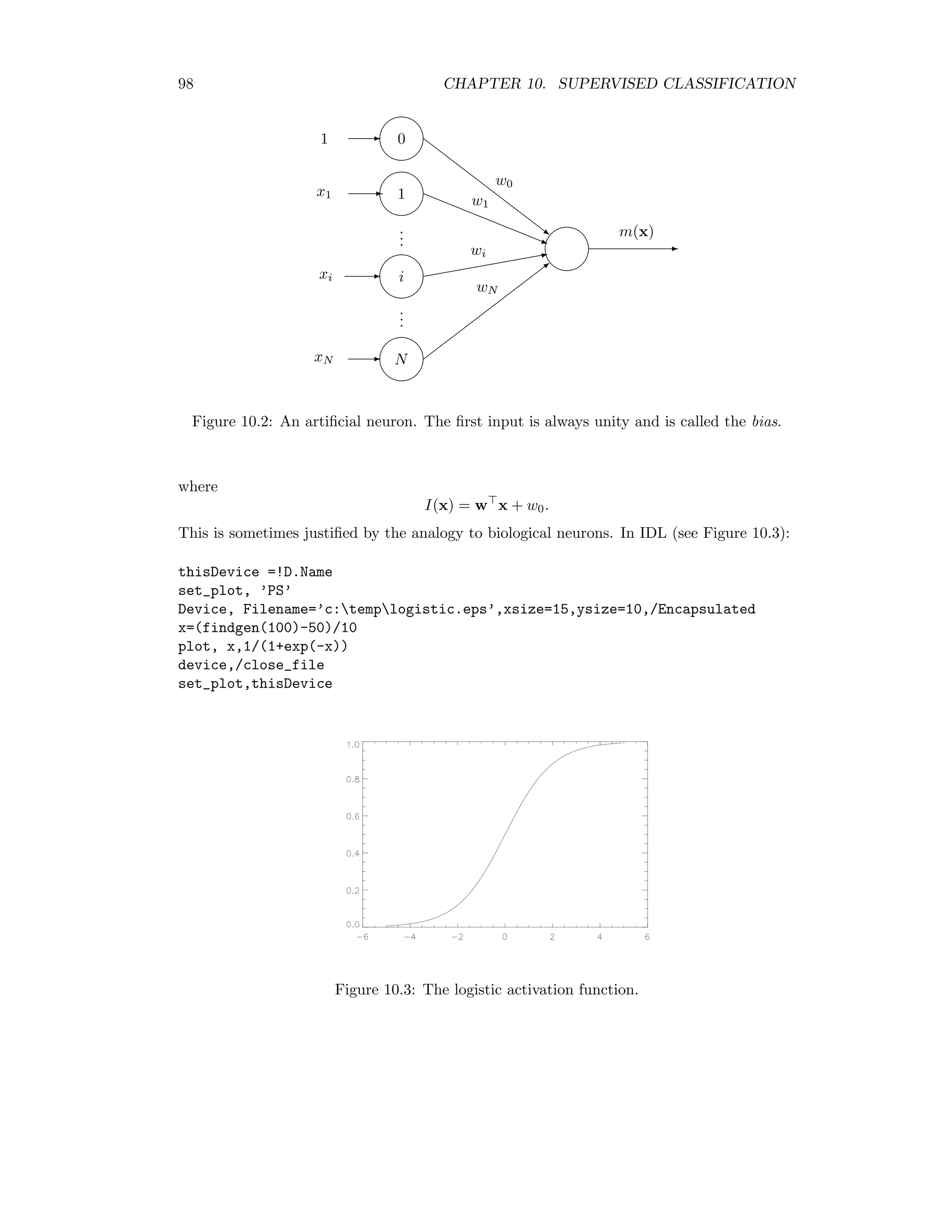
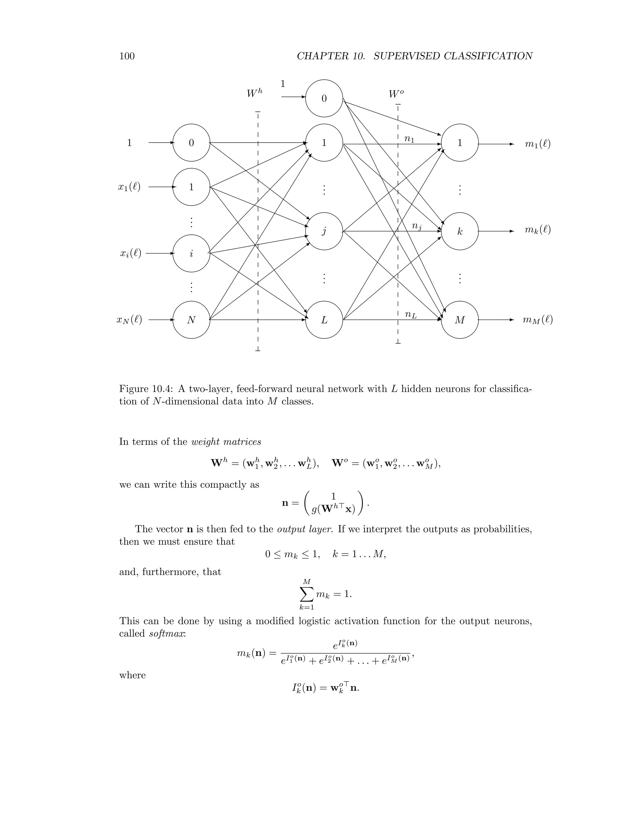
![94 CHAPTER 10. SUPERVISED CLASSIFICATION the the class ‘meadow’ is just as bad as classifying it as ‘urban area’, etc). The we can write λik = 1 − δik, . Thus any given misclassification (i = k) costs unity, and a correct classification (i = k) costs nothing. We then obtain from (10.3) L(Ci, x) = M k=1 P(Ck|x) − P(Ci|x) = 1 − P(Ci|x), i = 1 . . . M, (10.5) and from (10.4) the Bayes’ decision rule x ∈ Ci if P(Ci|x) P(Cj|x) for all j = 1 . . . M, j = i. (10.6) 10.2 Training data The selection of representative training data is the most difficult and critical part of the classification process. The standard procedure is to select training areas within the image which are representative of each class of interest. In the ENVI environment, these are entered as regions of interest (ROI’s), from which the training pixel vectors are generated. Note that some fraction of the representative data must be withheld for later accuracy assessment. These are the so-called test data, which are not used for training purposes in order not to bias the accuracy assessment. We’ll discuss their use in detail in later in this chapter. Suppose there are just two classes, that is M = 2. If we apply decision rule (10.6) to some measured pixel vector x, the probability of incorrectly classifying the pixel is r(x) = min[P(C1|x), P(C2|x)]. The Bayes error is defined to be the average of r(x) over all pixels, = r(x)p(x)dx = min[P(C1|x), P(C2|x)]p(x)dx = min[P(x|C1)P(C1), P(x|C2)P(C2)]dx, where we used Bayes rule in the last step. We can use the Bayes error as a measure of the separability of the two classes, the smaller the error, the better the separability. Calculating the Bayes error is difficult, but we can at least get an approximate upper bound as follows. First note that, for any a, b ≥ 0, min[a, b] ≤ aS b1−S , 0 ≤ S ≤ 1. For example, if a b, then the inequality can be written a ≤ a b a 1−S which is clearly true. Applying the inequality to the expression for the Bayes error, we get the so-called Chernoff bound ≤ u = P(C1)S P(C2)1−S P(x|C1)S P(x|C2)1−S dx.](https://image.slidesharecdn.com/mortonjohncanty-imageanalysisandpatternrecognitionforremotesensingwithalgorithmsinenvi-idl-190425063306/75/Morton-john-canty-image-analysis-and-pattern-recognition-for-remote-sensing-with-algorithms-in-envi-idl-109-2048.jpg)
![10.3. BAYES MAXIMUM LIKELIHOOD CLASSIFICATION 95 The best upper bound is then determined by minimizing u with respect to S. If we assume that P(x|C1) and P(x|C2) are normal distributions with Σ1 = Σ2, then the minimum occurs at S = 1/2. We get the Bhattacharyya bound B by using S = 1/2 also for the case where Σ1 = Σ2: B = P(C1)P(C2) P(x|C1)P(x|C2) dx. This integral can be evaluated explicitly. The result is B = P(C1)P(C2)e−B , where B is the Bhattacharyya distance given by B = 1 8 (µ2 − µ1) Σ1 + Σ2 2 −1 (µ2 − µ1) + 1 2 log Σ1 + Σ2 2 |Σ1||Σ2| . The first term is an “average Mahalinobis distance” (see below), the second term depends on the difference between the covariance matrices of the two classes. It vanishes when Σ1 = Σ2. Thus the first term gives the class separability due due the “distance” between the class means, while the second term gives the separability due to the difference in the covariance matrices. Finally, the Jeffries-Matusita distance measures separability of two classes on a scale [0 − 2] in terms of B: J = 2(1 − e−B ). (10.7) The ENVI menu command Basic Tools/Region of Interest/Compute ROI Separability calculates Jeffries-Matusita distances between all pairs of classes defined by a given set of ROIs. 10.3 Bayes Maximum likelihood classification Consider again Bayes’ rule: P(Ci|x) = P(x|Ci)P(Ci) P(x) where P(Ci), i = 1 . . . M, are a priori probabilities and where P(x) is given by P(x) = M j=1 P(x|Cj)P(Cj). Since P(x) is independent of i, we can write the decision rule (10.6) as x ∈ Ci if P(x|Ci)P(Ci) P(x|Cj)P(Cj) for all j = 1 . . . M, j = i. Now we make two simplifying assumptions: first, that all the a priori probabilities are equal, second, that the measured feature vectors from class Ci have been sampled from a multivariate normal distribution, that is, that they satisfy P(x|Ci) = 1 (2π)N/2|Σi|1/2 exp − 1 2 (x − µi) Σ−1 i (x − µi) . (10.8)](https://image.slidesharecdn.com/mortonjohncanty-imageanalysisandpatternrecognitionforremotesensingwithalgorithmsinenvi-idl-190425063306/75/Morton-john-canty-image-analysis-and-pattern-recognition-for-remote-sensing-with-algorithms-in-envi-idl-110-2048.jpg)
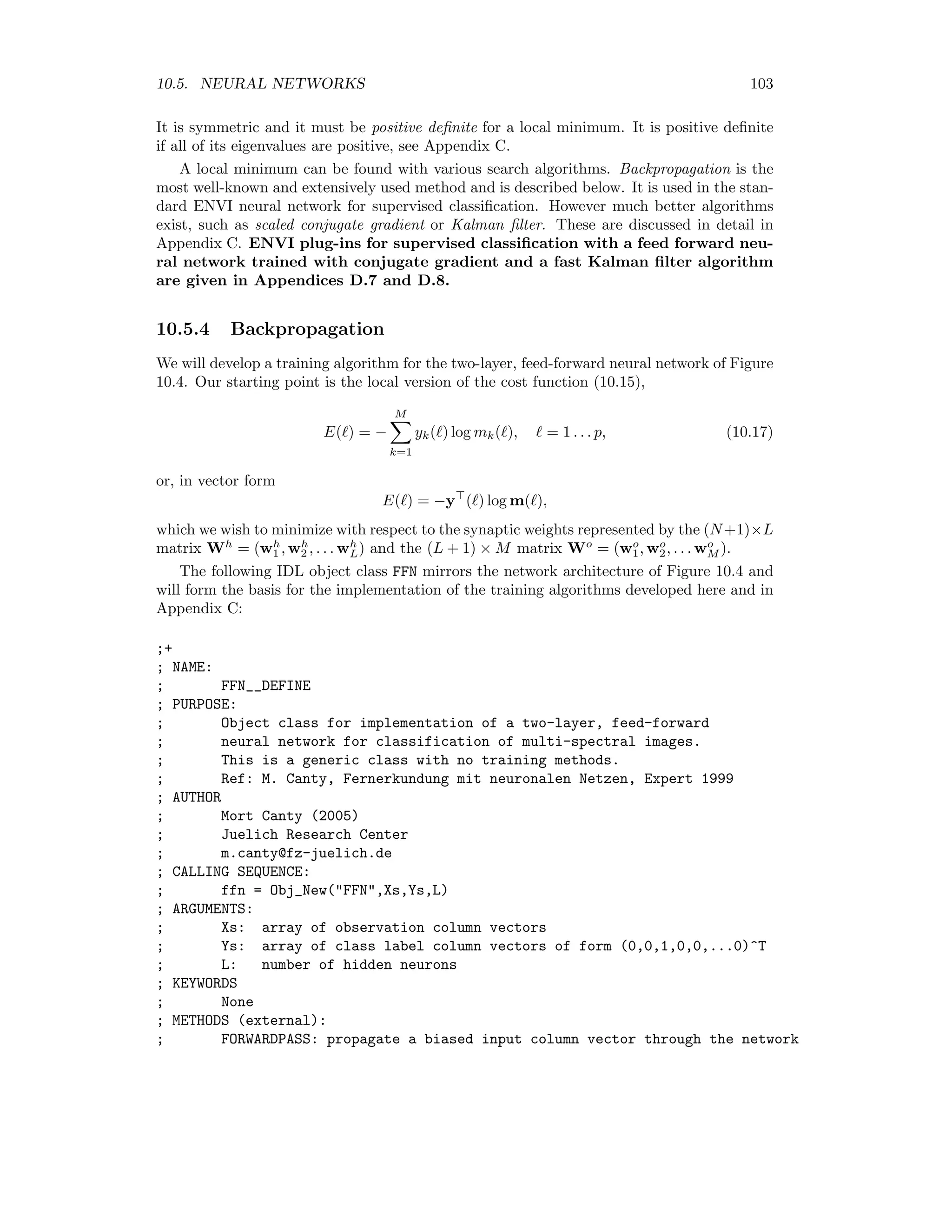
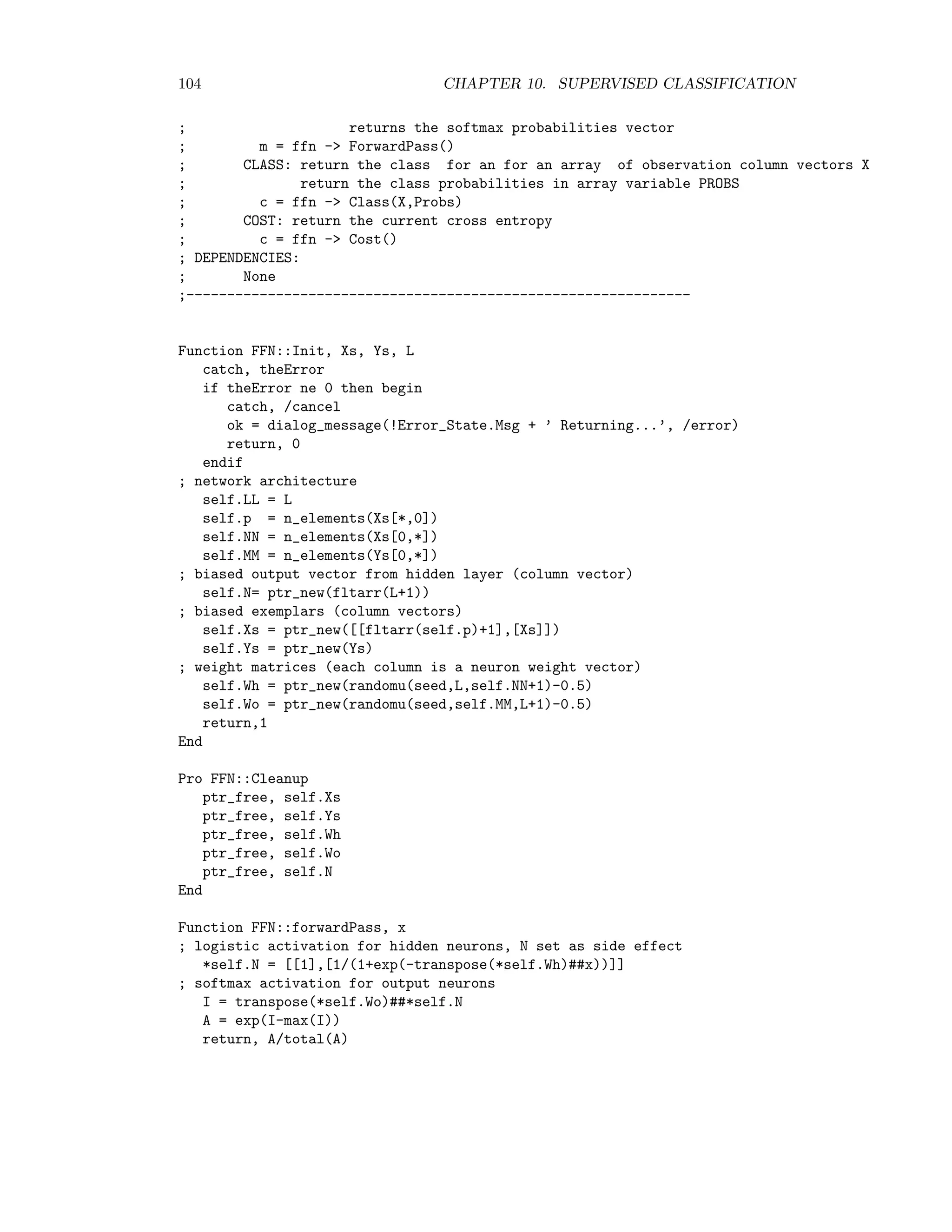
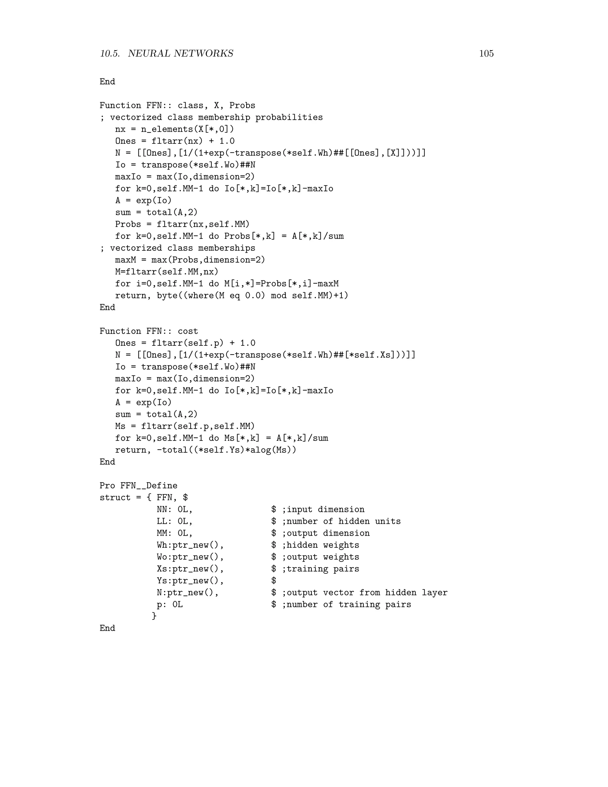
![10.5. NEURAL NETWORKS 99 There is also a statistical justification, however [Bis95]. Suppose two classes in two- dimensional feature space are normally distributed with Σ1 = Σ2 = I, P(x|Ck) ∼ 1 2π exp( −|x − µk|2 2 ), k = 1, 2. Then we have P(C1|x) = P(x|C1)P(C1) P(x|C1)P(C1) + P(x|C2)P(C2) = 1 1 + P(x|C2)P(C2)/P(x|C1)P(C1) = 1 1 + exp(−1 2 [(x − µ2)2 − (x − µ1)2])(P(C2)/P(C1)) . With the substitution e−a = (P(C2)/P(C1)) we get P(C1|x) = 1 1 + exp(−1 2 [|x − µ2|2 − |x − µ1|2] − a) = 1 1 + exp(−w x − w0) = 1 1 + e−I(x) = m(x). Here we made the additional substitutions w = µ1 − µ2 w0 = − 1 2 |µ1|2 + 1 2 |µ2|2 + a. Thus we expect that the output of the neuron will not only discriminate between the two classes, but also that it will approximate the posterior class membership probability P(C1|x). 10.5.1 The feed-forward network In order to discriminate any number of classes, multilayer feed-forward networks are often used, see Figure 10.4. In this figure, the input signal is the N + 1-component vector x( ) = (1, x1( ) . . . xN ( )) for training sample , which is fed simultaneously to the so-called hidden layer consisting of L neurons. These in turn determine the L + 1-component vector n(x) = (1, n1(x) . . . nL(x)) according to nj(x) = g(Ih j (x)), j = 1 . . . L, with Ih j (x) = wh j x, where wh is the hidden weight vector for the jth neuron wh = (wh 0 , wh 1 . . . wh L) .](https://image.slidesharecdn.com/mortonjohncanty-imageanalysisandpatternrecognitionforremotesensingwithalgorithmsinenvi-idl-190425063306/75/Morton-john-canty-image-analysis-and-pattern-recognition-for-remote-sensing-with-algorithms-in-envi-idl-114-2048.jpg)
![10.5. NEURAL NETWORKS 101 To quote Bishop [Bis95], “ ... such networks can approximate arbitrarily well any functional continu- ous mapping from one finite dimensional space to another, provided the number L of hidden units is sufficiently large. An important corollary of this result is, that in the context of a classification problem, networks with sigmoidal non- linearities and two layers of weights can approximate any decision boundary to arbitrary accuracy. More generally, the capability of such networks to approx- imate general smooth functions allows them to model posterior probabilities of class membership.” 10.5.2 Cost functions We haven’t yet considered the correct choice of synaptic weights. This procedure is called training the network. The training data can be represented as the set of labelled pairs {(x( ), y( )) | = 1 . . . p}, where y( ) = (0, 0 . . . 0, 1, 0 . . . 0) is an M-dimensional vector of zeroes, with a “1” at the kth position to indicate that x( ) belongs to class Ck. An intuitive training criterion is then the quadratic cost function E(Wh , Wo ) = 1 2 p =1 y( ) − m( ) 2 . (10.13) We must adjust the network weights so as to minimize E. Equivalently we can minimize the local cost functions E( ) := 1 2 y( ) − m( ) 2 , = 1 . . . p. (10.14) An alternative cost function can be obtained with the following argument: Choose the synaptic weights so as to maximize the probability of observing the training data: P(x( ), y( )) = P(y( ) | x( ))P(x( )) → max . The neural network predicts the posterior class membership probability, which we can write as P(y( ) | x( )) = M k=1 [ mk(x( )) ]yk( ) . For example: P((1, 0 . . . 0) |x) = m1(x)1 m2(x)0 smM (x)0 = m1(x). Therefore we wish to maximize M k=1 [ mk(x(i)) ]yk(i) P(x( ))](https://image.slidesharecdn.com/mortonjohncanty-imageanalysisandpatternrecognitionforremotesensingwithalgorithmsinenvi-idl-190425063306/75/Morton-john-canty-image-analysis-and-pattern-recognition-for-remote-sensing-with-algorithms-in-envi-idl-116-2048.jpg)
![104 CHAPTER 10. SUPERVISED CLASSIFICATION ; returns the softmax probabilities vector ; m = ffn - ForwardPass() ; CLASS: return the class for an for an array of observation column vectors X ; return the class probabilities in array variable PROBS ; c = ffn - Class(X,Probs) ; COST: return the current cross entropy ; c = ffn - Cost() ; DEPENDENCIES: ; None ;-------------------------------------------------------------- Function FFN::Init, Xs, Ys, L catch, theError if theError ne 0 then begin catch, /cancel ok = dialog_message(!Error_State.Msg + ’ Returning...’, /error) return, 0 endif ; network architecture self.LL = L self.p = n_elements(Xs[*,0]) self.NN = n_elements(Xs[0,*]) self.MM = n_elements(Ys[0,*]) ; biased output vector from hidden layer (column vector) self.N= ptr_new(fltarr(L+1)) ; biased exemplars (column vectors) self.Xs = ptr_new([[fltarr(self.p)+1],[Xs]]) self.Ys = ptr_new(Ys) ; weight matrices (each column is a neuron weight vector) self.Wh = ptr_new(randomu(seed,L,self.NN+1)-0.5) self.Wo = ptr_new(randomu(seed,self.MM,L+1)-0.5) return,1 End Pro FFN::Cleanup ptr_free, self.Xs ptr_free, self.Ys ptr_free, self.Wh ptr_free, self.Wo ptr_free, self.N End Function FFN::forwardPass, x ; logistic activation for hidden neurons, N set as side effect *self.N = [[1],[1/(1+exp(-transpose(*self.Wh)##x))]] ; softmax activation for output neurons I = transpose(*self.Wo)##*self.N A = exp(I-max(I)) return, A/total(A)](https://image.slidesharecdn.com/mortonjohncanty-imageanalysisandpatternrecognitionforremotesensingwithalgorithmsinenvi-idl-190425063306/75/Morton-john-canty-image-analysis-and-pattern-recognition-for-remote-sensing-with-algorithms-in-envi-idl-119-2048.jpg)
![10.5. NEURAL NETWORKS 105 End Function FFN:: class, X, Probs ; vectorized class membership probabilities nx = n_elements(X[*,0]) Ones = fltarr(nx) + 1.0 N = [[Ones],[1/(1+exp(-transpose(*self.Wh)##[[Ones],[X]]))]] Io = transpose(*self.Wo)##N maxIo = max(Io,dimension=2) for k=0,self.MM-1 do Io[*,k]=Io[*,k]-maxIo A = exp(Io) sum = total(A,2) Probs = fltarr(nx,self.MM) for k=0,self.MM-1 do Probs[*,k] = A[*,k]/sum ; vectorized class memberships maxM = max(Probs,dimension=2) M=fltarr(self.MM,nx) for i=0,self.MM-1 do M[i,*]=Probs[*,i]-maxM return, byte((where(M eq 0.0) mod self.MM)+1) End Function FFN:: cost Ones = fltarr(self.p) + 1.0 N = [[Ones],[1/(1+exp(-transpose(*self.Wh)##[*self.Xs]))]] Io = transpose(*self.Wo)##N maxIo = max(Io,dimension=2) for k=0,self.MM-1 do Io[*,k]=Io[*,k]-maxIo A = exp(Io) sum = total(A,2) Ms = fltarr(self.p,self.MM) for k=0,self.MM-1 do Ms[*,k] = A[*,k]/sum return, -total((*self.Ys)*alog(Ms)) End Pro FFN__Define struct = { FFN, $ NN: 0L, $ ;input dimension LL: 0L, $ ;number of hidden units MM: 0L, $ ;output dimension Wh:ptr_new(), $ ;hidden weights Wo:ptr_new(), $ ;output weights Xs:ptr_new(), $ ;training pairs Ys:ptr_new(), $ N:ptr_new(), $ ;output vector from hidden layer p: 0L $ ;number of training pairs } End](https://image.slidesharecdn.com/mortonjohncanty-imageanalysisandpatternrecognitionforremotesensingwithalgorithmsinenvi-idl-190425063306/75/Morton-john-canty-image-analysis-and-pattern-recognition-for-remote-sensing-with-algorithms-in-envi-idl-120-2048.jpg)

![110 CHAPTER 10. SUPERVISED CLASSIFICATION progressbar-Destroy return endif ; select exemplar pair at random ell = long(self.p*randomu(seed)) x=(*self.Xs)[ell,*] y=(*self.Ys)[ell,*] ; send it through the network m=self-forwardPass(x) ; determine the deltas d_o = y - m d_h = (*self.N*(1-*self.N)*(*self.Wo##d_o))[1:self.LL] ; d_h is now a row vector ; update the synaptic weights inc_o = eta*(*self.N##transpose(d_o)) inc_h = eta*(x##d_h) *self.Wo = *self.Wo + inc_o + alpha*inc_o1 *self.Wh = *self.Wh + inc_h + alpha*inc_h1 inc_o1 = inc_o inc_h1 = inc_h ; record cost history if iter mod 100 eq 0 then begin (*self.cost_array)[iter100]=alog10(self-cost()) iter100 = iter100+1 progressbar-Update,iter*100/self.iterations,text=strtrim(iter,2) plot,*self.cost_array,xrange=[0,iter100],color=0,background=’FFFFFF’XL,$ xtitle=’Iterations/100)’,ytitle=’log(cross entropy)’ end iter=iter+1 endrep until iter eq self.iterations progressbar-destroy End Pro FFNBP__Define struct = { FFNBP, $ cost_array: ptr_new(), $ iterations: 0L, $ Inherits FFN $ } End In the Train method, the training pairs are chosen at random, rather than cyclically as indicated in the backpropagation Algorithm. 10.6 Evaluation The rate of misclassification offers us a reasonable and obvious basis not only for evaluating the quality of classifiers, but also for their comparison, for example to compare the feed- forward network with Bayes maximum-likelihood. We shall characterize this rate in the following with the parameter θ. Through classification of test data which have not been](https://image.slidesharecdn.com/mortonjohncanty-imageanalysisandpatternrecognitionforremotesensingwithalgorithmsinenvi-idl-190425063306/75/Morton-john-canty-image-analysis-and-pattern-recognition-for-remote-sensing-with-algorithms-in-envi-idl-125-2048.jpg)
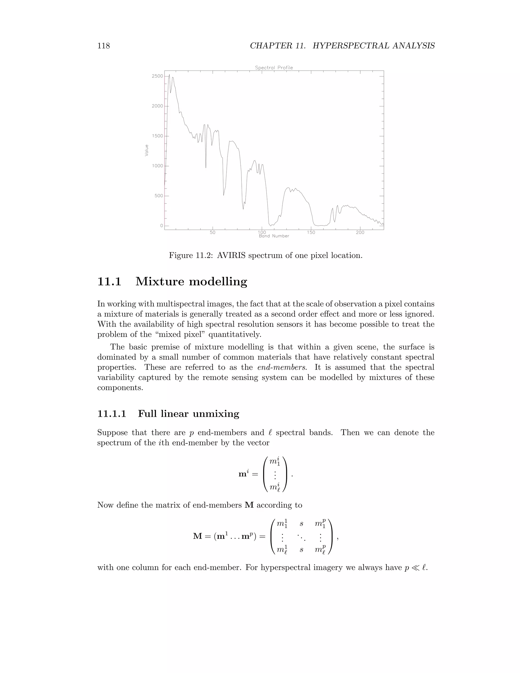
![112 CHAPTER 10. SUPERVISED CLASSIFICATION and the estimated standard deviation by ˆσ = y(n − y) n3 . (10.33) The random variable Y is binomially distributed. However for a sufficiently large number n of test data, the binomial distribution is well-approximated by the normal distribution. Mean and standard deviation are then sufficient to characterize the distribution function completely. 10.6.2 Model comparison A typical value for a misclassification rate is around θ ≈ 0.5. In order to claim that two values differ from one another significantly, they should lie at least about two standard deviations apart. If we wish to discriminate values separated by say 0.01, then ˆσ should be no greater than 0.005. From (10.32) this means 0.0052 ≈ 0.05(1 − 0.05) n , or n ≈ 2000. That’s quite a few. However since we are dealing with pixel data, such a number of test pixels – assuming sufficient training areas are available – is quite realistic. If training and test data are in fact at a premium, there exist efficient alternatives1 to the simple train-and-test philosophy presented here. However, since they are generally quite computer-intensive, we won’t consider them further. In order to express the claim that classifier A is better than classifier B more precisely, we can formulate an hypothesis test. The individual misclassification rates are approximately normally distributed. If they are also independent we can construct a test statistic S given by S = YA/n − YB/n + θA − θB var(YA/n − YB/n) = YA/n − YB/n + θA − θB var(YA/n) + var(YB/n) . We can then use S to decide between the null hypothesis H0 : θA = θB, i.e., the two classifiers are equivalent, and the alternative hypothesis H1 : θA θB or θA θB, i.e. one of the two methods is better. Thus under H0 we have S ∼ N(0, 1). We choose a decision threshold ±Zα/2 which cor- responds to a probability α of an error of the first kind. With this probability the null hypothesis will be rejected although it is in fact true, see Figure 10.6. In fact the strict independence of the misclassification rates θA and θB is not given, since they are determined with the same set of test data. The above hypothesis test with the statistic S is therefore too conservative. For dependence we have namely var(YA/n − YB/n) = var(YA/n) + var(YB/n) − 2cov(YA/n, YB/n), 1The buzz-words here are Cross-Validation and Bootstrapping, see [WK91], Chapter 2, for an excellent introduction.](https://image.slidesharecdn.com/mortonjohncanty-imageanalysisandpatternrecognitionforremotesensingwithalgorithmsinenvi-idl-190425063306/75/Morton-john-canty-image-analysis-and-pattern-recognition-for-remote-sensing-with-algorithms-in-envi-idl-127-2048.jpg)
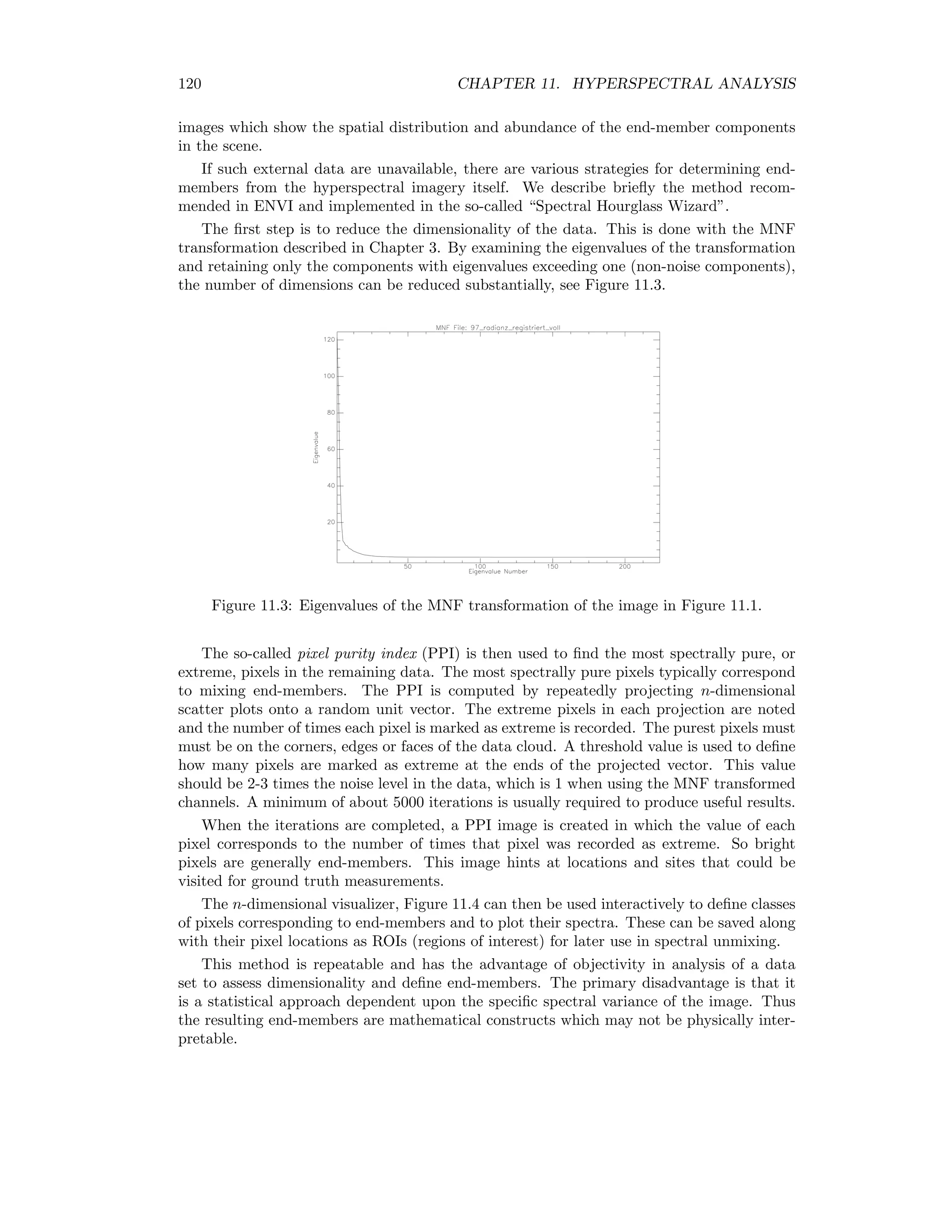
![114 CHAPTER 10. SUPERVISED CLASSIFICATION We expect that θ ¯AB 1, that is, var(Y ¯AB) ≈ nθ ¯AB = Y ¯AB . The same goes for YA ¯B. For a sufficiently large number of test observationss, the random variables Y ¯AB − Y ¯AB Y ¯AB and YA¯B − YA¯B YA¯B are thus approximately standard normally distributed. Under the null hypothesis (equivalence of the two classifiers), the expectation values of Y ¯AB and YA ¯B satisfy Y ¯AB = YA ¯B =: Y . Therefore we form the test statistic S = (Y ¯AB − Y )2 Y + (YA ¯B − Y )2 Y . This statistic, being the sum squares of approximately normally distributed random vari- ables, is chi-square distributed, see Chapter 2. Let y ¯AB and yA ¯B be the number of events actually measured. Then we estimate Y as ˆY = y ¯AB + yA ¯B 2 and determine our test statistic as ˆS = (y ¯AB − y ¯AB+yA ¯B 2 )2 y ¯AB+yA ¯B 2 + (yA ¯B − y ¯AB+yA ¯B 2 )2 y ¯AB+yA ¯B 2 . With a little algebra we get ˆS = (y ¯AB − yA ¯B)2 y ¯AB + yA ¯B , (10.34) the so-called McNemar statistic. It is chi-square distributed with one degree of freedom, see for example [Sie65]. A so-called continuity correction is usually made to (10.34) and S written as ˆS = (|y ¯AB − yA ¯B| − 1)2 y ¯AB + yA ¯B . But there are still reservations! We can only conclude that one classifier is or is not superior, relative to the common set of training data. We haven’t taken into account the variability of the training data, which were sampled just once from their underlying distri- butions, only that of the test data. If one or both of the classifiers is a neural network, we have also not considered the variability of the neural network training procedure with re- spect to the random initialization of the synaptic weights. All this constitutes an extremely computation-intensive task [Rip96]. 10.6.3 Confusion matrices The confusion matrix for M classes is defined as C = c11 c12 s c1M c21 c22 s c2M ... ... ... ... cM1 cM2 s cMM ](https://image.slidesharecdn.com/mortonjohncanty-imageanalysisandpatternrecognitionforremotesensingwithalgorithmsinenvi-idl-190425063306/75/Morton-john-canty-image-analysis-and-pattern-recognition-for-remote-sensing-with-algorithms-in-envi-idl-129-2048.jpg)
![10.6. EVALUATION 115 where cij is the number of test pixels from class Ci which are classified as Cj. The misclas- sification rate is ˆθ = y n = n − M i=1 cii n = n − Tr C n and only takes into account of the diagonal elements of the confusion matrix. The Kappa-coefficient κ make use of all the matrix elements. It is defined as follows: κ = correct classifications − chance correct classifications 1 − chance correct classifications For a purely randomly labeled test pixel, the proportion of correct classifications is approx- imately M i=1 ci ci n2 , where ci = M j=1 cij, ci = M j=1 cji. Hence an estimate of the Kappa coefficient is ˆκ = i cii n − i cici n2 1 − i cici n2 . (10.35) Again, the Kappa coefficient alone tells us little about the quality of the classifier. We require its standard deviation. This can be calculated in the large sample limit n → ∞ to be [BFH75] ˆσˆκ = 1 n θ1(1 − θ1) (1 − θ2)2 + 2(1 − θ1)(2θ1θ2 − θ3) (1 − θ3)3 + (1 − θ1)2 (θ4 − 4θ2 2) (1 − θ2)4 , (10.36) where θ1 = M i=1 cii θ2 = M i=1 cici θ3 = M i=1 cii(ci + ci) θ4 = M i,j=1 cij(cj + ci)2 .](https://image.slidesharecdn.com/mortonjohncanty-imageanalysisandpatternrecognitionforremotesensingwithalgorithmsinenvi-idl-190425063306/75/Morton-john-canty-image-analysis-and-pattern-recognition-for-remote-sensing-with-algorithms-in-envi-idl-130-2048.jpg)

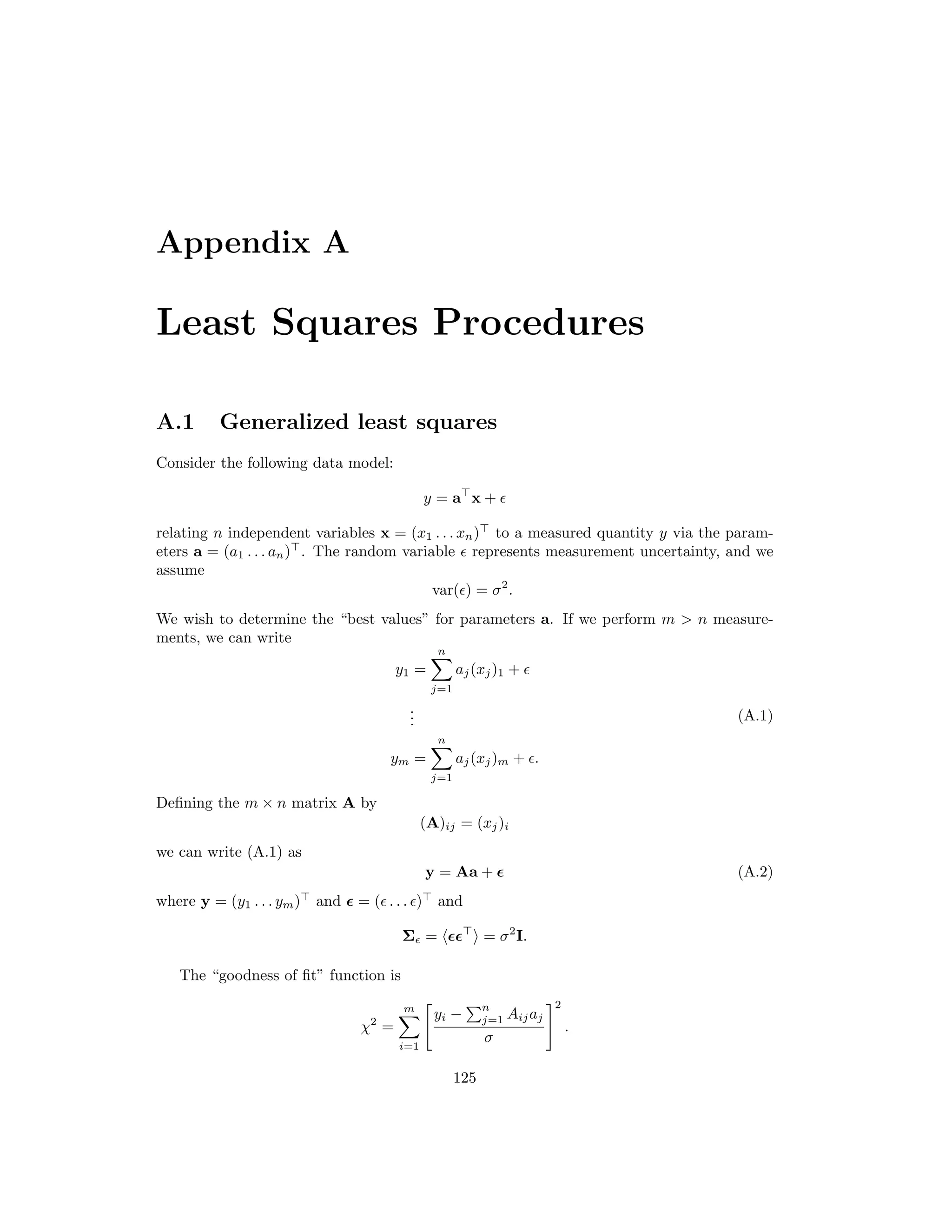
![11.1. MIXTURE MODELLING 119 The measured signal g is modelled as a linear combination of end-members plus a residual noise term: g = α1m1 + . . . + αpmp + n = Mα + n. The residual n is assumed to be normally distributed with covariance matrix Σn = σ2 1 0 s 0 0 σ2 2 s 0 ... ... ... ... 0 0 s σ2 . The standardized residual is Σ−1/2 n n and the square of the standardized residual is (Σ−1/2 n n) (Σ−1/2 n n) = n Σ−1 n n. The mixing coefficients are determined my minimizing this quantity with respect to α under the condition that they sum to unity. The corresponding Lagrange function is L = n Σ−1 n n − 2λ( p i=1 αi − 1) = (g − Mα) Σ−1 n (g − Mα) − 2λ( p i=1 αi − 1) . Solving the set of equations ∂L ∂α = 0 ∂L ∂λ = 0 we obtain the solution α = (M Σ−1 n M)−1 (M Σ−1 n g − λ1p) α1p = 1, (11.1) where 1p = (1, 1 . . . 1) . The first equation determines the mixing coefficients in terms of known quantities and λ. The second equation can be used to eliminate λ. 11.1.2 Unconstrained linear unmixing If we work with MNF-projected data (see next section) then we can assume that Σn = σ2 I. If furthermore we ignore the constraint on α (i.e. λ = 0), then (11.1) reduces to α = [(M M)−1 M ]g. The expression in square brackets is the pseudoinverse of the matrix M, see Chapter 1. 11.1.3 Intrinsic end-members and pixel purity If a spectral library for all of the p end-members in M is available, the mixture coefficients can be calculated directly. The primary result of the spectral mixture analysis is the fraction](https://image.slidesharecdn.com/mortonjohncanty-imageanalysisandpatternrecognitionforremotesensingwithalgorithmsinenvi-idl-190425063306/75/Morton-john-canty-image-analysis-and-pattern-recognition-for-remote-sensing-with-algorithms-in-envi-idl-134-2048.jpg)
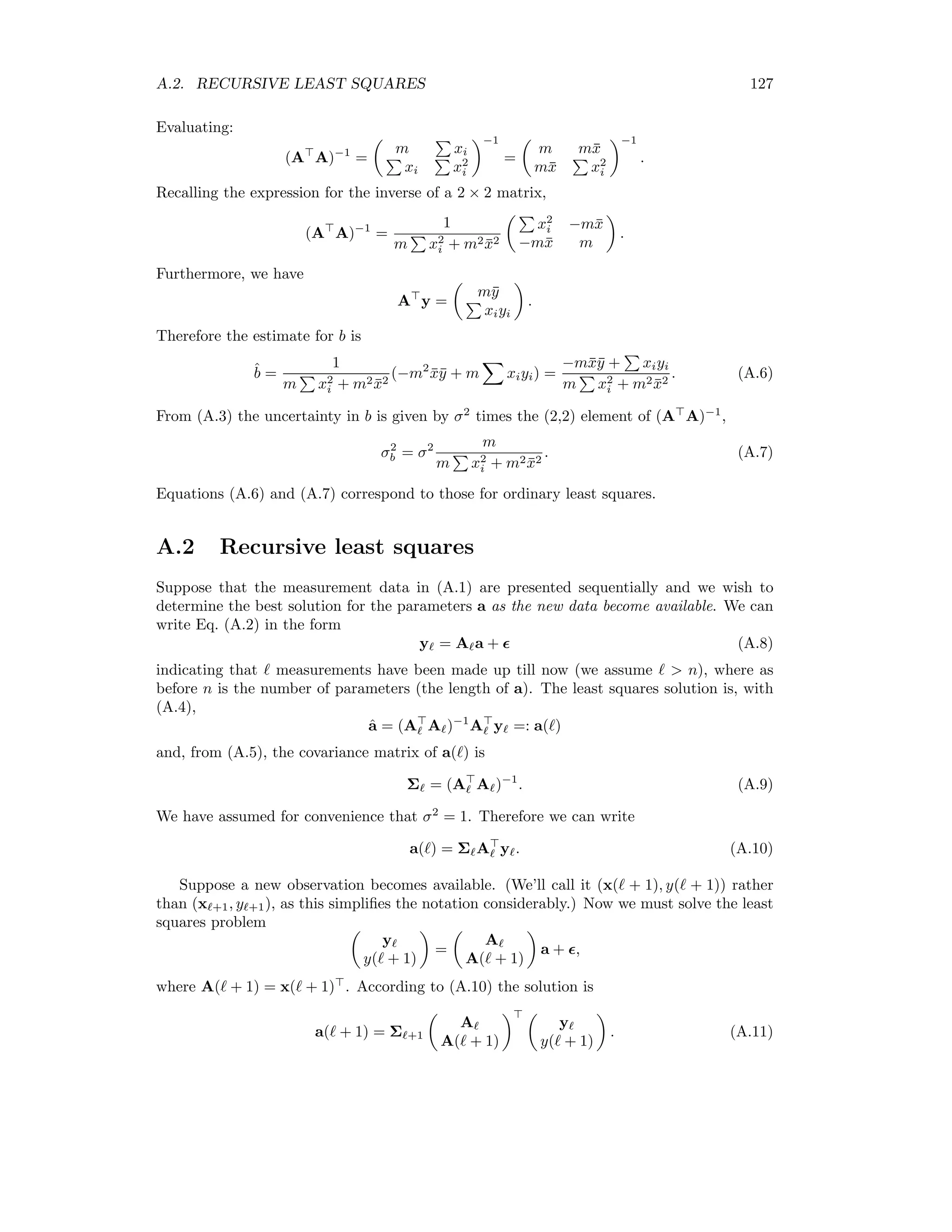
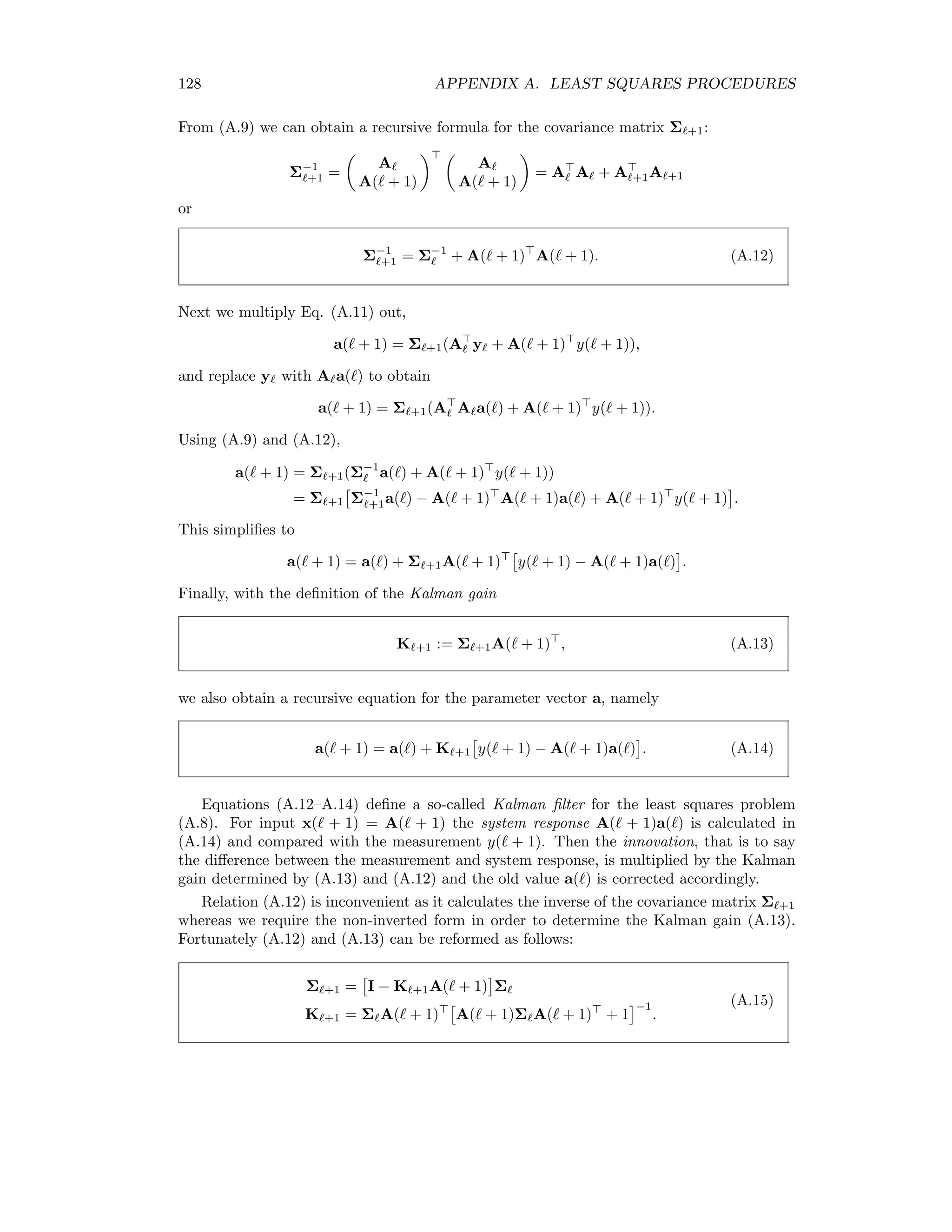
![122 CHAPTER 11. HYPERSPECTRAL ANALYSIS print, ’---------------------------------’ infile=dialog_pickfile(filter=’*.dat’,/read) ; read in cluster centers openr,lun,infile,/get_lun readf,lun,num_channels ; number of spectral channels readf,lun,K ; number of cluster centers Ms=fltarr(num_channels,K) readf,lun,Ms Us=transpose(Ms) print,’Cluster centers (in the columns)’ print,Us centers=indgen(K) print,’enter undesired centers as 1 (e.g. 0 1 1 0 0 ...)’ read,centers U = Us[where(centers),*] print,’Subspace U’ print,U Identity = fltarr(num_channels,num_channels) for i=0,num_channels-1 do Identity[i,i]=1.0 P = Identity - U##invert(transpose(U)##U,/double)##transpose(U) print,’projection matrix:’ print, P envi_select, title=’Choose multispectral image for projection’, $ fid=fid, dims=dims,pos=pos if (fid eq -1) then goto, done num_cols = dims[2]+1 num_lines = dims[4]+1 num_pixels = (num_cols*num_lines) if (num_channels ne n_elements(pos)) then begin print,’image dimensions are incorrect, aborting ...’ goto, done end image=fltarr(num_pixels,num_channels) for i=0,num_channels-1 do $ image[*,i]=envi_get_data(fid=fid,dims=dims,pos=pos[i])+0.0 print,’projecting ...’ ; do the projection image = P ## image out_array = bytarr(num_cols,num_lines,num_channels) for i = 0,num_channels-1 do out_array[*,*,i] = $ bytscl(reform(image[*,i],num_cols,num_lines,/overwrite)) base = widget_auto_base(title=’OSP Output’)](https://image.slidesharecdn.com/mortonjohncanty-imageanalysisandpatternrecognitionforremotesensingwithalgorithmsinenvi-idl-190425063306/75/Morton-john-canty-image-analysis-and-pattern-recognition-for-remote-sensing-with-algorithms-in-envi-idl-137-2048.jpg)
![11.2. ORTHOGONAL SUBSPACE PROJECTION 123 sb = widget_base(base, /row, /frame) wp = widget_outfm(sb, uvalue=’outf’, /auto) result = auto_wid_mng(base) if (result.accept eq 0) then begin print, ’Output cancelled’ goto, done endif if (result.outf.in_memory eq 1) then begin envi_enter_data, out_array print, ’Result written to memory’ endif else begin openw, unit, result.outf.name, /get_lun band_names=strarr(num_channels) for i=0,num_channels-1 do begin writeu, unit, out_array[*,*,i] band_names[i]=’OSP component ’ + string(i+1) endfor envi_setup_head ,fname=result.outf.name, ns=num_samples, $ nl=num_lines, nb=num_channels $ ,data_type=1, interleave=0, /write $ ,bnames=band_names $ ,descrip=’OSP’ print, ’File created ’, result.outf.name close, unit endelse done: print,’done.’ end](https://image.slidesharecdn.com/mortonjohncanty-imageanalysisandpatternrecognitionforremotesensingwithalgorithmsinenvi-idl-190425063306/75/Morton-john-canty-image-analysis-and-pattern-recognition-for-remote-sensing-with-algorithms-in-envi-idl-138-2048.jpg)
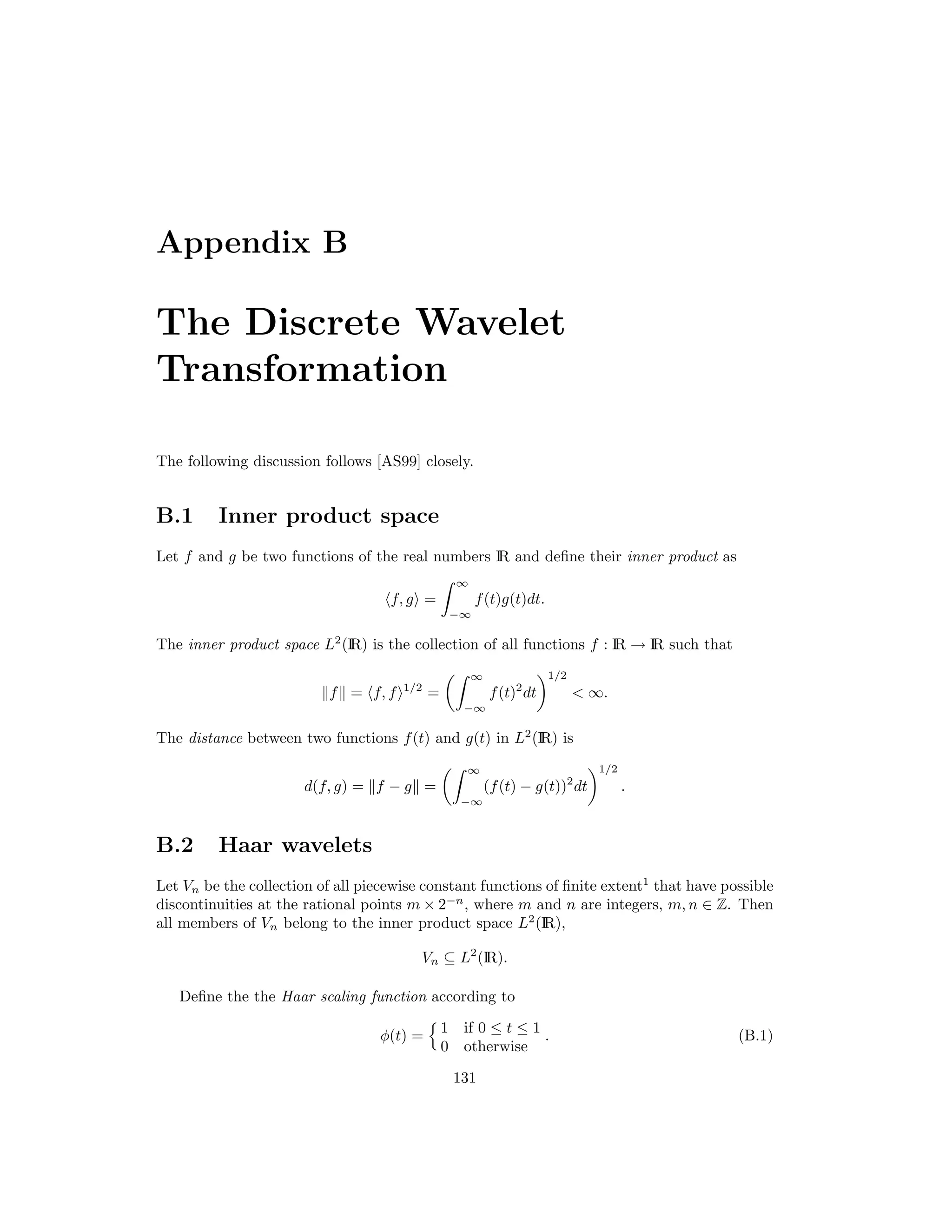
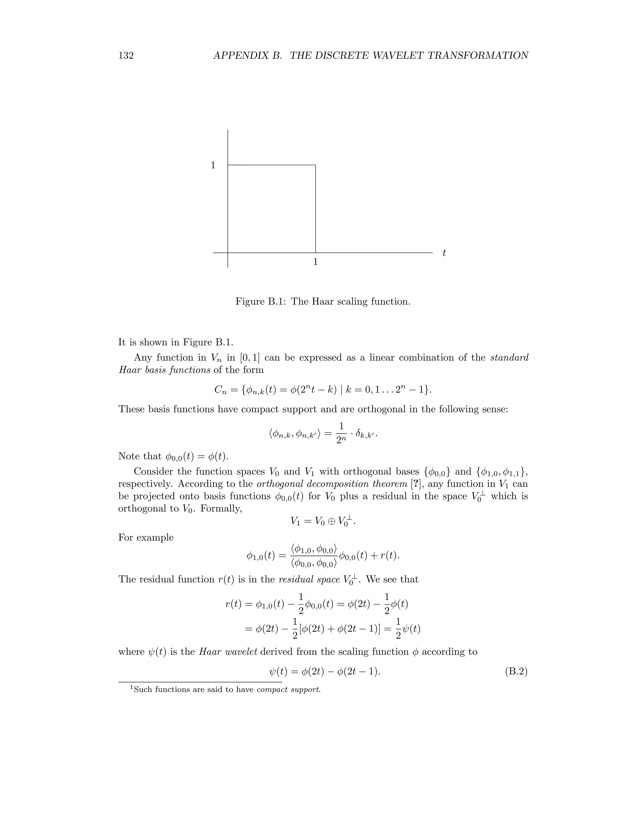

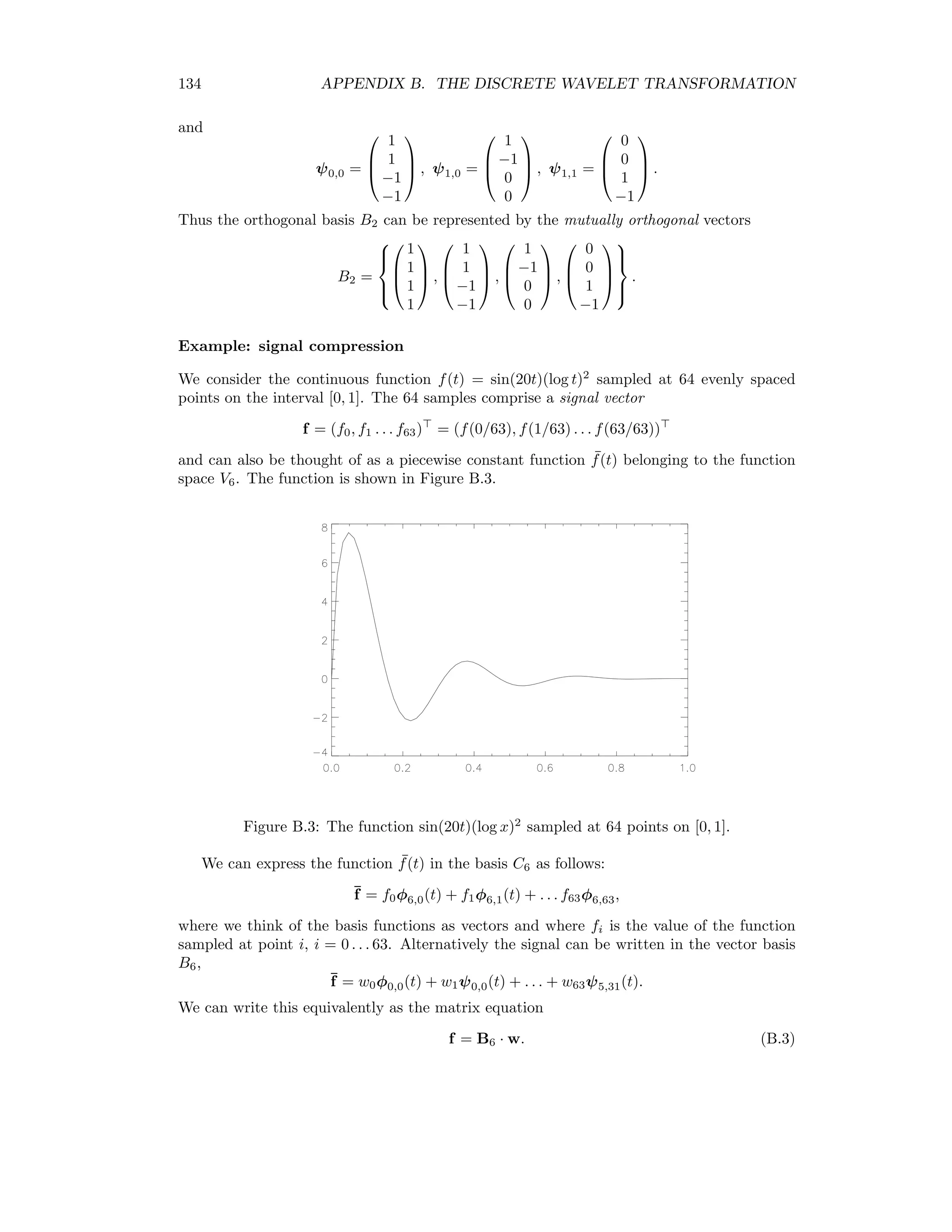
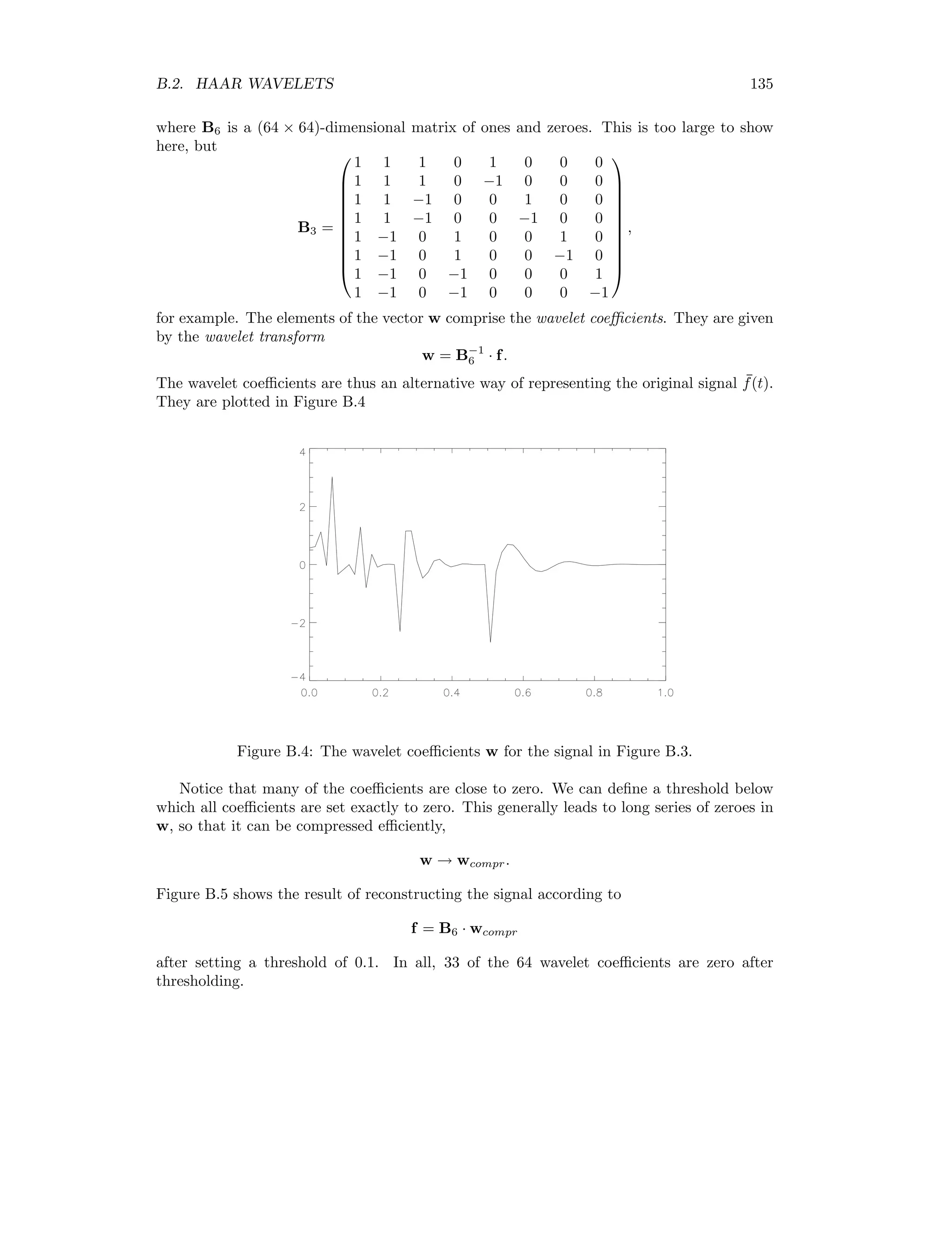
![A.3. ORTHOGONAL REGRESSION 129 To see this, first of all note that the second equation in (A.15) is a consequence of the first equation and (A.13). Therefore it suffices to show that the first equation is indeed the inverse of (A.12): Σ +1Σ−1 +1 = I − K +1A( + 1) Σ Σ−1 +1 = I − K +1A( + 1) + I − K +1A( + 1) Σ A( + 1) A( + 1) = I − K +1A( + 1) + Σ A( + 1) A( + 1) − K +1A( + 1)Σ A( + 1) A( + 1). The second equality above follows from (A.12). But from the second equation in (A.15) we have K +1A( + 1)Σ A( + 1) = Σ A( + 1) − K +1 and therefore Σ +1Σ−1 +1 = I − K +1A( + 1) + Σ A( + 1) A( + 1) − (Σ A( + 1) − K +1)A( + 1) = I as required. A.3 Orthogonal regression In the model for ordinary least squares regression the xs are assumed to be error-free. In the calibration case where it is arbitrary what we call the reference variable and what we call the uncalibrated variable to be normalized, we should allow for error in both x and y. If we impose the model1 yi − i = a + b(xi − δi), i = 1 . . . m (A.16) with and δ as uncorrelated, white, Gaussian noise terms with mean zero and equal variances σ2 , we get for the estimator of b, [KS79], ˆb = (s2 yy − s2 xx) + (s2 yy − s2 xx)2 + 4s2 xy 2sxy (A.17) with s2 yy = 1 m n i=1 (yi − ¯y)2 (A.18) and the remaining quantities defined in the section immediately above. The estimator for a is ˆa = ¯y − ˆb¯x. (A.19) According to [Pat77, Bil89] we get for the dispersion matrix of the vector (ˆa,ˆb) σ2ˆb(1 + ˆb2 ) msxy ¯x2 (1 + ˆτ) + sxy/ˆb −¯x(1 + ˆτ) −¯x(1 + ˆτ) 1 + ˆτ (A.20) with ˆτ = σ2ˆb (1 + ˆb2)sxy (A.21) 1The model in equation (A.16) is often referred to as a linear functional relationship in the literature.](https://image.slidesharecdn.com/mortonjohncanty-imageanalysisandpatternrecognitionforremotesensingwithalgorithmsinenvi-idl-190425063306/75/Morton-john-canty-image-analysis-and-pattern-recognition-for-remote-sensing-with-algorithms-in-envi-idl-144-2048.jpg)
![130 APPENDIX A. LEAST SQUARES PROCEDURES and where σ2 can be replaced by ˆσ2 = m (n − 2)(1 + ˆb2) (s2 yy − 2ˆbsxy + ˆb2 s2 xx), (A.22) see [KS79]. It can be shown that estimators of a and b can be calculated by means of the elements in the eigenvector corresponding to the smallest eigenvalue of the dispersion matrix of the m by 2 data matrix with a vector of the xs in the first column and a vector of the ys in the second column, [KS79]. This can be used to perform orthogonal regression in higher dimensions, i.e., when we have, for example, more x variables than the one variable we have here.](https://image.slidesharecdn.com/mortonjohncanty-imageanalysisandpatternrecognitionforremotesensingwithalgorithmsinenvi-idl-190425063306/75/Morton-john-canty-image-analysis-and-pattern-recognition-for-remote-sensing-with-algorithms-in-envi-idl-145-2048.jpg)
![Appendix B The Discrete Wavelet Transformation The following discussion follows [AS99] closely. B.1 Inner product space Let f and g be two functions of the real numbers IR and define their inner product as f, g = ∞ −∞ f(t)g(t)dt. The inner product space L2 (IR) is the collection of all functions f : IR → IR such that f = f, f 1/2 = ∞ −∞ f(t)2 dt 1/2 ∞. The distance between two functions f(t) and g(t) in L2 (IR) is d(f, g) = f − g = ∞ −∞ (f(t) − g(t))2 dt 1/2 . B.2 Haar wavelets Let Vn be the collection of all piecewise constant functions of finite extent1 that have possible discontinuities at the rational points m × 2−n , where m and n are integers, m, n ∈ Z. Then all members of Vn belong to the inner product space L2 (IR), Vn ⊆ L2 (IR). Define the the Haar scaling function according to φ(t) = 1 if 0 ≤ t ≤ 1 0 otherwise . (B.1) 131](https://image.slidesharecdn.com/mortonjohncanty-imageanalysisandpatternrecognitionforremotesensingwithalgorithmsinenvi-idl-190425063306/75/Morton-john-canty-image-analysis-and-pattern-recognition-for-remote-sensing-with-algorithms-in-envi-idl-146-2048.jpg)
![132 APPENDIX B. THE DISCRETE WAVELET TRANSFORMATION 1 1 t Figure B.1: The Haar scaling function. It is shown in Figure B.1. Any function in Vn in [0, 1] can be expressed as a linear combination of the standard Haar basis functions of the form Cn = {φn,k(t) = φ(2n t − k) | k = 0, 1 . . . 2n − 1}. These basis functions have compact support and are orthogonal in the following sense: φn,k, φn,k = 1 2n · δk,k . Note that φ0,0(t) = φ(t). Consider the function spaces V0 and V1 with orthogonal bases {φ0,0} and {φ1,0, φ1,1}, respectively. According to the orthogonal decomposition theorem [?], any function in V1 can be projected onto basis functions φ0,0(t) for V0 plus a residual in the space V ⊥ 0 which is orthogonal to V0. Formally, V1 = V0 ⊕ V ⊥ 0 . For example φ1,0(t) = φ1,0, φ0,0 φ0,0, φ0,0 φ0,0(t) + r(t). The residual function r(t) is in the residual space V ⊥ 0 . We see that r(t) = φ1,0(t) − 1 2 φ0,0(t) = φ(2t) − 1 2 φ(t) = φ(2t) − 1 2 [φ(2t) + φ(2t − 1)] = 1 2 ψ(t) where ψ(t) is the Haar wavelet derived from the scaling function φ according to ψ(t) = φ(2t) − φ(2t − 1). (B.2) 1Such functions are said to have compact support.](https://image.slidesharecdn.com/mortonjohncanty-imageanalysisandpatternrecognitionforremotesensingwithalgorithmsinenvi-idl-190425063306/75/Morton-john-canty-image-analysis-and-pattern-recognition-for-remote-sensing-with-algorithms-in-envi-idl-147-2048.jpg)
![134 APPENDIX B. THE DISCRETE WAVELET TRANSFORMATION and ψ0,0 = 1 1 −1 −1 , ψ1,0 = 1 −1 0 0 , ψ1,1 = 0 0 1 −1 . Thus the orthogonal basis B2 can be represented by the mutually orthogonal vectors B2 = 1 1 1 1 , 1 1 −1 −1 , 1 −1 0 0 , 0 0 1 −1 . Example: signal compression We consider the continuous function f(t) = sin(20t)(log t)2 sampled at 64 evenly spaced points on the interval [0, 1]. The 64 samples comprise a signal vector f = (f0, f1 . . . f63) = (f(0/63), f(1/63) . . . f(63/63)) and can also be thought of as a piecewise constant function ¯f(t) belonging to the function space V6. The function is shown in Figure B.3. Figure B.3: The function sin(20t)(log x)2 sampled at 64 points on [0, 1]. We can express the function ¯f(t) in the basis C6 as follows: ¯f = f0φ6,0(t) + f1φ6,1(t) + . . . f63φ6,63, where we think of the basis functions as vectors and where fi is the value of the function sampled at point i, i = 0 . . . 63. Alternatively the signal can be written in the vector basis B6, ¯f = w0φ0,0(t) + w1ψ0,0(t) + . . . + w63ψ5,31(t). We can write this equivalently as the matrix equation f = B6 · w. (B.3)](https://image.slidesharecdn.com/mortonjohncanty-imageanalysisandpatternrecognitionforremotesensingwithalgorithmsinenvi-idl-190425063306/75/Morton-john-canty-image-analysis-and-pattern-recognition-for-remote-sensing-with-algorithms-in-envi-idl-149-2048.jpg)
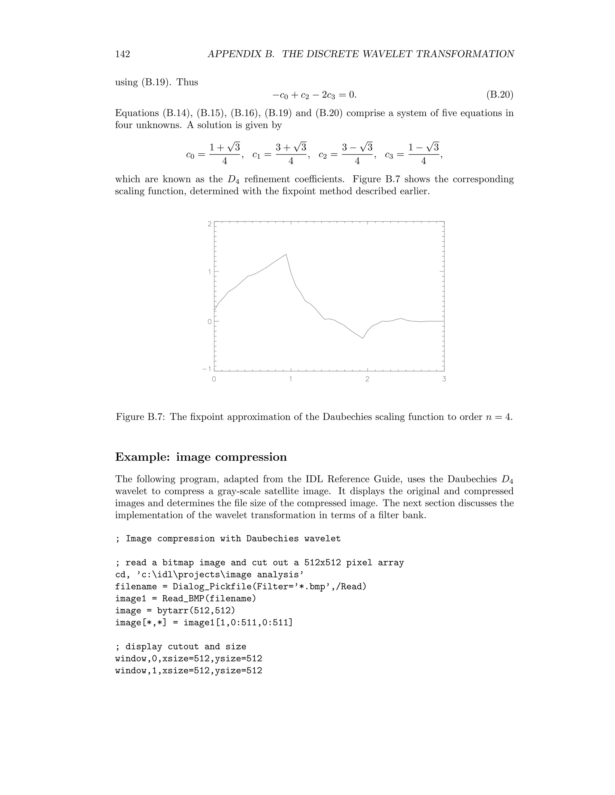
![136 APPENDIX B. THE DISCRETE WAVELET TRANSFORMATION Figure B.5: The reconstructed signal after thresholding at 0.1. The following program illustrates the above steps in IDL: ; generate a signal vector t=findgen(64)/63 f=sin(20*t)*alog(t)*alog(t) f[0]=0 ; output as EPS file thisDevice =!D.Name set_plot, ’PS’ Device, Filename=’c:tempsignal.eps’,xsize=15,ysize=10,/Encapsulated plot,t,f,color=1,background=’FFFFFF’XL device,/close_file ; read in basis B6 filename = Dialog_Pickfile(Filter=’*.dat’,/Read) openR,lun,filename,/get_lun B6 = fltarr(64,64) ReadF, lun, B6 ; do the wavelet transform and display w=invert(B6)##f Device, Filename=’c:tempwavelet_coeff.eps’,xsize=15,ysize=10,/Encapsulated plot,t,w,color=1,background=’FFFFFF’XL ; display compressed signal w( where(abs(w) lt 0.1) )=0.0 Device, Filename=’c:temprecon_signal.eps’,xsize=15,ysize=10,/Encapsulated plot,t,w,color=1,background=’FFFFFF’XL device,/close_file set_plot, thisDevice end](https://image.slidesharecdn.com/mortonjohncanty-imageanalysisandpatternrecognitionforremotesensingwithalgorithmsinenvi-idl-190425063306/75/Morton-john-canty-image-analysis-and-pattern-recognition-for-remote-sensing-with-algorithms-in-envi-idl-151-2048.jpg)
![B.3. MULTI-RESOLUTION ANALYSIS 137 B.3 Multi-resolution analysis So far we have considered only functions on the interval [0, 1] with basis functions φn,k(t) = φ(2n t − k), k = 1 . . . 2n − 1. We can extend this to functions defined on all real numbers IR in a straightforward way. For example {φ(t − k) | k ∈ Z} is a basis for the space V0 of all piecewise constant functions with compact support (finite extent) having possible breaks at integer values. More generally, a basis for the set Vn of piecewise constant functions with possible breaks at m × 2−n and compact support is {φ(2n t − k) | k ∈ Z}. We can even allow n 0. For example n = −1 means that the possible breaks are at even integer values. We can think of the collection of nested subspaces of piecewise constant functions . . . ⊆ V−1 ⊆ V0 ⊆ V1 ⊆ V2 ⊆ . . . ⊆ L2 (IR), as being generated by the Haar scaling function φ. This collection is called a multiresolution analysis (MRA). A general MRA must have the following properties: 1. V = n∈Z Vn is dense in L2 (IR), that is, for any function f ∈ L2 (IR) there exists a series of functions, one in each Vn, which converges to f. This is true of the Haar MRA, see Figure 2.7 for example. 2. The separation property: I = n∈Z Vn = {0}. For the Haar MRA, this means that any function in I must be piecewise constant on all intervals. The only function in L2 (IR) with this property and compact support is f(t) = 0, so the separation property is satisfied. 3. The function f(t) ∈ Vn if and only if f(2−n t) ∈ V0. In the Haar MRA, if f(t) ∈ V1 then it is piecewise constant on intervals of length 1/2. Therefore the function f(2−1 t) is piecewise constant on intervals of length 1, that is f(2−1 t) ∈ V0, etc. 4. The scaling function φ is an orthonormal basis for the function space V0, i.e. φ(t − k), φ(t − k ) = δkk . This is of course the case for the Haar scaling function. In the following, we will think of φ(t) as any scaling function which generates an MRA in the above sense. Since {φ(t − k) | k ∈ Z} is an orthonormal basis for V0, it follows that {φ(2t − k) | k ∈ Z} is an orthogonal basis for V1. That is, let f(t) ∈ V1. Then by property 3, f(t/2) ∈ V0 and f(t/2) = k akφ(t − k) ⇒ f(t) = k akφ(2t − k). In particular, since φ(t) ∈ V0 ⊆ V1, we have the dilation equation φ(t) = k ckφ(2t − k). (B.4)](https://image.slidesharecdn.com/mortonjohncanty-imageanalysisandpatternrecognitionforremotesensingwithalgorithmsinenvi-idl-190425063306/75/Morton-john-canty-image-analysis-and-pattern-recognition-for-remote-sensing-with-algorithms-in-envi-idl-152-2048.jpg)
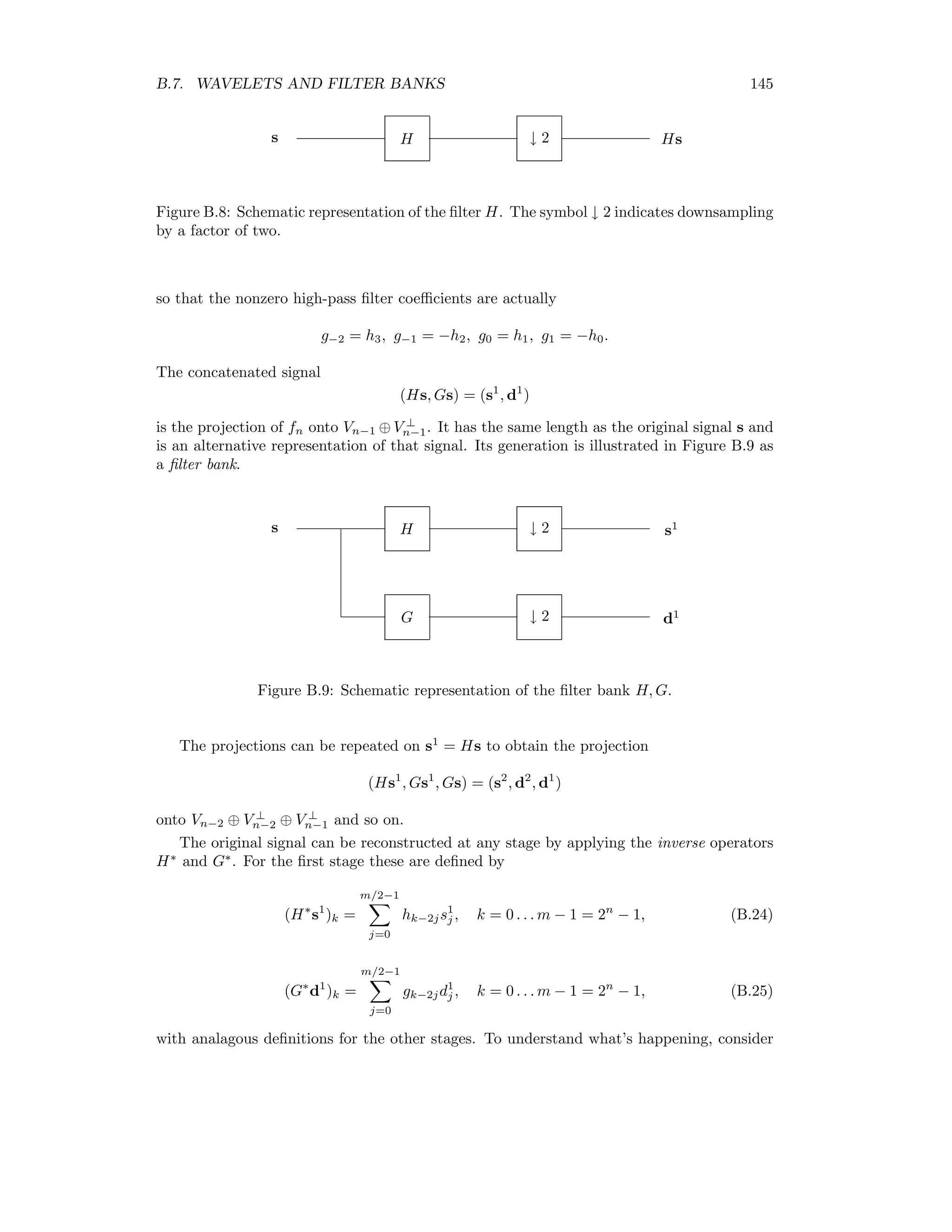
![B.4. FIXPOINT WAVELET APPROXIMATION 139 as a pointwise approximation of φ. Here is a recursive IDL program to approximate any scaling function with 4 refinement coefficients: ffunction f, t, i common refinement, c0,c1,c2,c3 if (i eq 0) then if (t eq 0) then return, 1.0 else return, 0.0 $ else return, c0*f(2*t,i-1)+c1*f(2*t-1,i-1)+c2*f(2*t-2,i-1)+c3*f(2*t-3,i-1) end common refinement, c0,c1,c2,c3 ; refinement coefficients for Haar scaling function ; c0=1 c1=1 c2=0 c3=0 ; refinement coefficients for Daubechies scaling function c0=(1+sqrt(3))/4 c1=(3+sqrt(3))/4 c2=(3-sqrt(3))/4 c3=(1-sqrt(3))/4 ; fourth order approximation n=4 t = findgen(3*2^n) ff=fltarr(3*2^n) for i=0,3*2^n-1 do ff[i]=f(t[i]/2^n,n) ; output as EPS file thisDevice =!D.Name set_plot, ’PS’ Device, Filename=’c:tempdaubechies_approx.eps’,xsize=15,ysize=10,/Encapsulated plot,t/2^n,ff,yrange=[-1,2],color=1,background=’FFFFFF’XL device,/close_file set_plot,thisDevice end Figure B.6: The fixpoint approximation of the Haar scaling function to order n = 4. Figure B.6 shows the result of n=4 iterations using the refinement coefficients c0 = c1 = 1, c2 = c3 = 0 for the Haar scaling function.](https://image.slidesharecdn.com/mortonjohncanty-imageanalysisandpatternrecognitionforremotesensingwithalgorithmsinenvi-idl-190425063306/75/Morton-john-canty-image-analysis-and-pattern-recognition-for-remote-sensing-with-algorithms-in-envi-idl-154-2048.jpg)
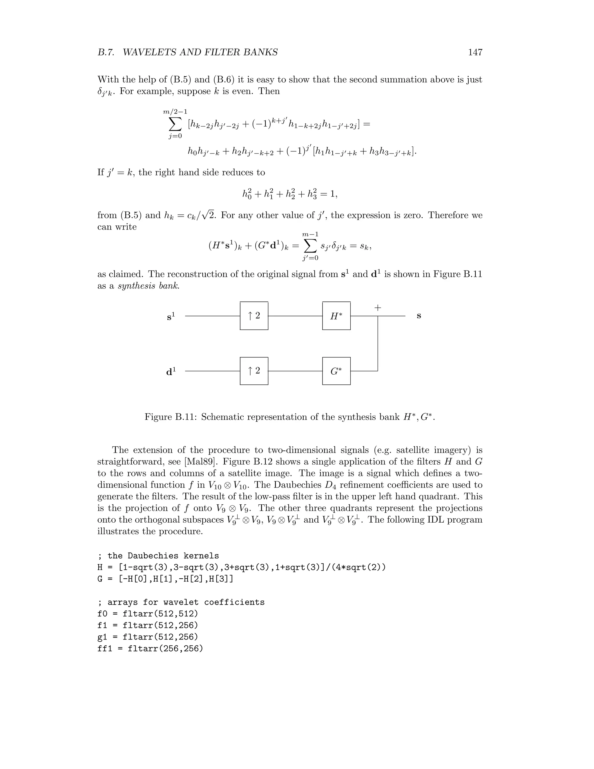
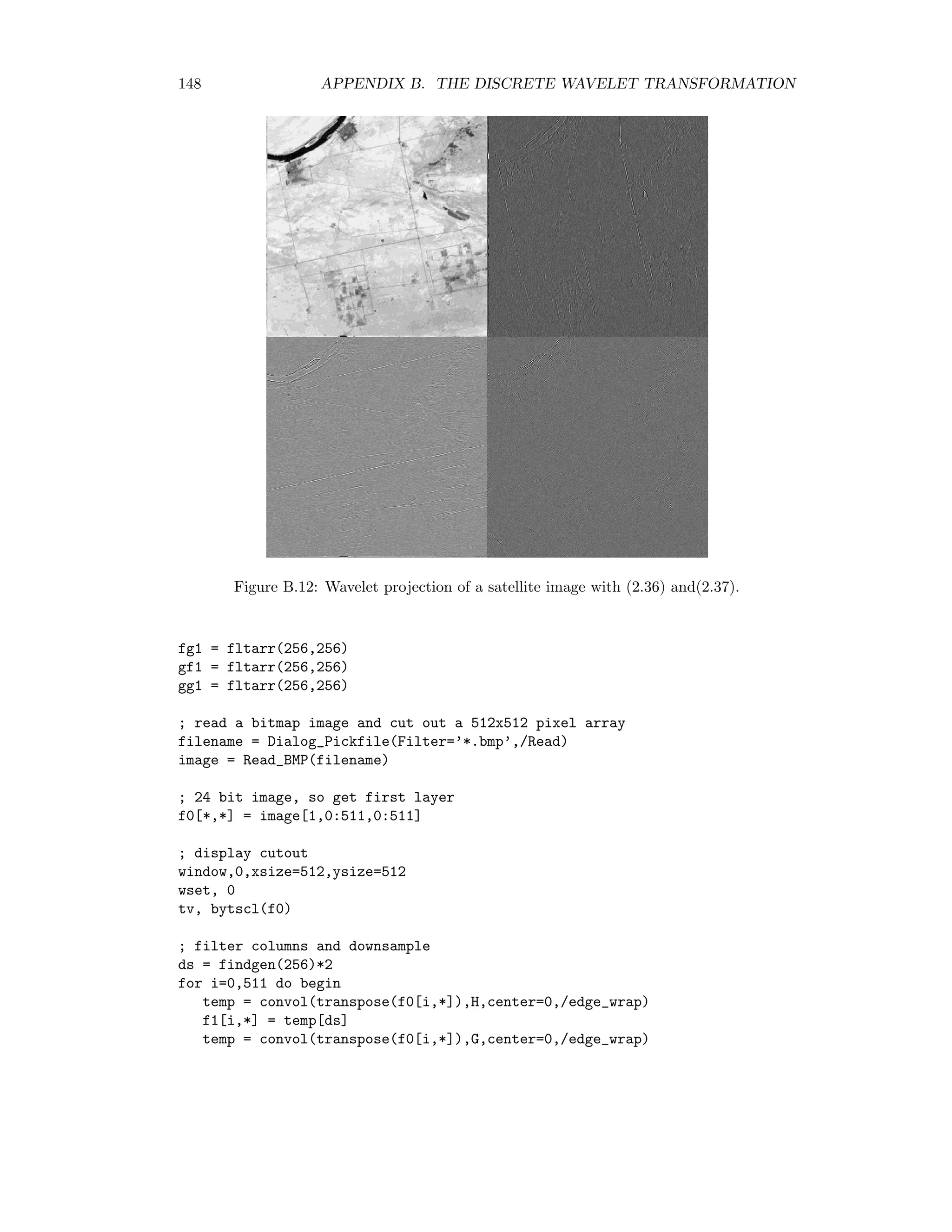
![142 APPENDIX B. THE DISCRETE WAVELET TRANSFORMATION using (B.19). Thus −c0 + c2 − 2c3 = 0. (B.20) Equations (B.14), (B.15), (B.16), (B.19) and (B.20) comprise a system of five equations in four unknowns. A solution is given by c0 = 1 + √ 3 4 , c1 = 3 + √ 3 4 , c2 = 3 − √ 3 4 , c3 = 1 − √ 3 4 , which are known as the D4 refinement coefficients. Figure B.7 shows the corresponding scaling function, determined with the fixpoint method described earlier. Figure B.7: The fixpoint approximation of the Daubechies scaling function to order n = 4. Example: image compression The following program, adapted from the IDL Reference Guide, uses the Daubechies D4 wavelet to compress a gray-scale satellite image. It displays the original and compressed images and determines the file size of the compressed image. The next section discusses the implementation of the wavelet transformation in terms of a filter bank. ; Image compression with Daubechies wavelet ; read a bitmap image and cut out a 512x512 pixel array cd, ’c:idlprojectsimage analysis’ filename = Dialog_Pickfile(Filter=’*.bmp’,/Read) image1 = Read_BMP(filename) image = bytarr(512,512) image[*,*] = image1[1,0:511,0:511] ; display cutout and size window,0,xsize=512,ysize=512 window,1,xsize=512,ysize=512](https://image.slidesharecdn.com/mortonjohncanty-imageanalysisandpatternrecognitionforremotesensingwithalgorithmsinenvi-idl-190425063306/75/Morton-john-canty-image-analysis-and-pattern-recognition-for-remote-sensing-with-algorithms-in-envi-idl-157-2048.jpg)
![B.7. WAVELETS AND FILTER BANKS 143 wset, 0 tv, bytscl(image) print, ’Size of original image is’, 512*512L, ’ bytes’ ; perform wavelet transform with D4 wavlet wtn_image = wtn(image, 4) ; convert to sparse array with threshold 20 and write to disk sparse_image = sprsin(wtn_image,thresh=20) write_spr, sparse_image, ’sparse.dat’ openr, 1, ’sparse.dat’ status = fstat(1) close, 1 print, ’Size of compressed image is’, status.size, ’ bytes’ ; reconstruct full array, do inverse wavelet transform and display wset,1 tv, bytscl(wtn(fulstr(sparse_image), 4, /inverse)) end B.7 Wavelets and filter banks In the case of the Haar wavelets we were able to carry out the wavelet transformation with vectors and matrices. In general, we can’t represent scaling functions in this way. In fact usually all that we have to work with are the refinement coefficients. So how can we perform the wavelet transformation? To answer this question, consider a row of pixels (s(0), s(1) . . . s(m − 1)) in a satellite image, where m = 2n , and the associated vector signal on [0, 1] given by s = (s0, s1 . . . sm−1) = (s(0/(m − 1)), s(1/(m − 1)) . . . s(1)) . In the MRA generated by a scaling function φ, such as D4, this signal defines a function fn(t) ∈ Vn on the interval [0, 1] according to fn(t) = m−1 j=0 sjφn,j = m−1 j=0 sjφ(2n t − j). (B.21) Assume that the basis functions are appropriately normalized. The projection of fn(t) onto Vn−1 is then fn−1(t) = m/2−1 k=0 fn, φ(2n−1 t − k) φ(2n−1 t − k) = m/2−1 k=0 (Hs)kφ(2n−1 t − k), where Hs = fn, φ(2n−1 t) , fn, φ(2n−1 t − 1) . . . fn, φ(2n−1 t − m/2 − 1)](https://image.slidesharecdn.com/mortonjohncanty-imageanalysisandpatternrecognitionforremotesensingwithalgorithmsinenvi-idl-190425063306/75/Morton-john-canty-image-analysis-and-pattern-recognition-for-remote-sensing-with-algorithms-in-envi-idl-158-2048.jpg)
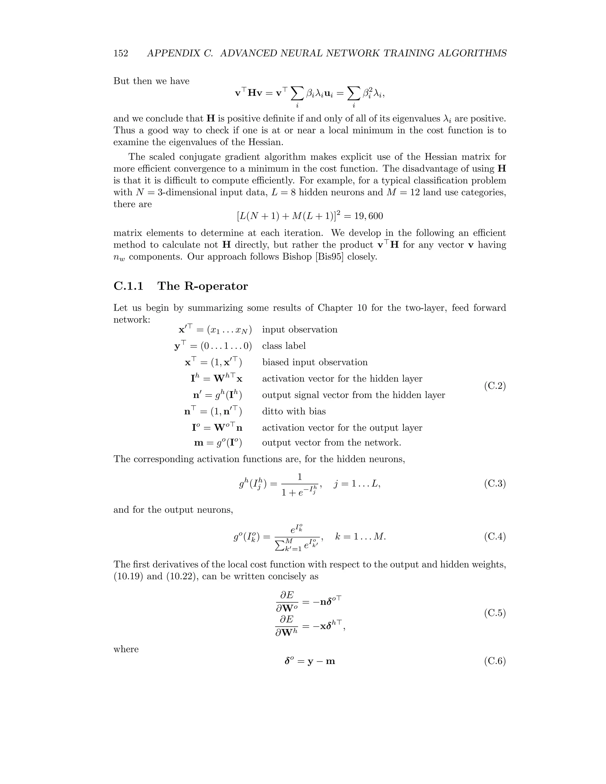
![146 APPENDIX B. THE DISCRETE WAVELET TRANSFORMATION the elements of the filtered signal (B.24). These are (H∗ s1 )0 = h0s1 0 (H∗ s1 )1 = h1s1 0 (H∗ s1 )2 = h2s1 0 + h0s1 1 (H∗ s1 )3 = h3s1 0 + h1s1 1 (H∗ s1 )4 = h2s1 1 + h0s1 2 (H∗ s1 )5 = h3s1 1 + h1s1 2 ... This is just the convolution of the filter H∗ = (h0, h1, h2, h3) with the signal s1 0, 0, s1 1, 0, s1 2, 0 . . . s1 m/2−1, 0. This is called the upsampled signal. The filter (B.24) can be represented schematically as in Figure B.10. s1 H∗ s1↑ 2 H∗ Figure B.10: Schematic representation of the filter H∗ . The symbol ↑ 2 indicates upsampling by a factor of two. Equation (B.25) is interpreted in a similar way. Finally we add the two results to get the original signal: H∗ s1 + G∗ d1 = s. To see this, write the equation out for a particular value of k: (H∗ s1 )k + (G∗ d1 )k = m/2−1 j=0 hk−2j m−1 j =0 hj −2jsj + gk−2j m−1 j =0 gj −2jsj Combining terms and interchanging the summations, we get (H∗ s1 )k + (G∗ d1 )k = m−1 j =0 sj m/2−1 j=0 [hk−2jhj −2j + gk−2jgj −2j]. Now, using gk = (−1)k h1−k, (H∗ s1 )k + (G∗ d1 )k = m−1 j =0 sj m/2−1 j=0 [hk−2jhj −2j + (−1)k+j h1−k+2jh1−j +2j].](https://image.slidesharecdn.com/mortonjohncanty-imageanalysisandpatternrecognitionforremotesensingwithalgorithmsinenvi-idl-190425063306/75/Morton-john-canty-image-analysis-and-pattern-recognition-for-remote-sensing-with-algorithms-in-envi-idl-161-2048.jpg)
![B.7. WAVELETS AND FILTER BANKS 147 With the help of (B.5) and (B.6) it is easy to show that the second summation above is just δj k. For example, suppose k is even. Then m/2−1 j=0 [hk−2jhj −2j + (−1)k+j h1−k+2jh1−j +2j] = h0hj −k + h2hj −k+2 + (−1)j [h1h1−j +k + h3h3−j +k]. If j = k, the right hand side reduces to h2 0 + h2 1 + h2 2 + h2 3 = 1, from (B.5) and hk = ck/ √ 2. For any other value of j , the expression is zero. Therefore we can write (H∗ s1 )k + (G∗ d1 )k = m−1 j =0 sj δj k = sk, as claimed. The reconstruction of the original signal from s1 and d1 is shown in Figure B.11 as a synthesis bank. s1 ↑ 2 H∗ ↑ 2 G∗ s d1 + Figure B.11: Schematic representation of the synthesis bank H∗ , G∗ . The extension of the procedure to two-dimensional signals (e.g. satellite imagery) is straightforward, see [Mal89]. Figure B.12 shows a single application of the filters H and G to the rows and columns of a satellite image. The image is a signal which defines a two- dimensional function f in V10 ⊗ V10. The Daubechies D4 refinement coefficients are used to generate the filters. The result of the low-pass filter is in the upper left hand quadrant. This is the projection of f onto V9 ⊗ V9. The other three quadrants represent the projections onto the orthogonal subspaces V ⊥ 9 ⊗V9, V9 ⊗V ⊥ 9 and V ⊥ 9 ⊗V ⊥ 9 . The following IDL program illustrates the procedure. ; the Daubechies kernels H = [1-sqrt(3),3-sqrt(3),3+sqrt(3),1+sqrt(3)]/(4*sqrt(2)) G = [-H[0],H[1],-H[2],H[3]] ; arrays for wavelet coefficients f0 = fltarr(512,512) f1 = fltarr(512,256) g1 = fltarr(512,256) ff1 = fltarr(256,256)](https://image.slidesharecdn.com/mortonjohncanty-imageanalysisandpatternrecognitionforremotesensingwithalgorithmsinenvi-idl-190425063306/75/Morton-john-canty-image-analysis-and-pattern-recognition-for-remote-sensing-with-algorithms-in-envi-idl-162-2048.jpg)
![148 APPENDIX B. THE DISCRETE WAVELET TRANSFORMATION Figure B.12: Wavelet projection of a satellite image with (2.36) and(2.37). fg1 = fltarr(256,256) gf1 = fltarr(256,256) gg1 = fltarr(256,256) ; read a bitmap image and cut out a 512x512 pixel array filename = Dialog_Pickfile(Filter=’*.bmp’,/Read) image = Read_BMP(filename) ; 24 bit image, so get first layer f0[*,*] = image[1,0:511,0:511] ; display cutout window,0,xsize=512,ysize=512 wset, 0 tv, bytscl(f0) ; filter columns and downsample ds = findgen(256)*2 for i=0,511 do begin temp = convol(transpose(f0[i,*]),H,center=0,/edge_wrap) f1[i,*] = temp[ds] temp = convol(transpose(f0[i,*]),G,center=0,/edge_wrap)](https://image.slidesharecdn.com/mortonjohncanty-imageanalysisandpatternrecognitionforremotesensingwithalgorithmsinenvi-idl-190425063306/75/Morton-john-canty-image-analysis-and-pattern-recognition-for-remote-sensing-with-algorithms-in-envi-idl-163-2048.jpg)
![B.7. WAVELETS AND FILTER BANKS 149 g1[i,*] = temp[ds] endfor ; filter rows and downsample for i=0,255 do begin temp = convol(f1[*,i],H,center=0,/edge_wrap) ff1[*,i] = temp[ds] temp = convol(f1[*,i],G,center=0,/edge_wrap) fg1[*,i] = temp[ds] temp = convol(g1[*,i],H,center=0,/edge_wrap) gf1[*,i] = temp[ds] temp = convol(g1[*,i],G,center=0,/edge_wrap) gg1[*,i] = temp[ds] endfor f0[0:255,256:511]=bytscl(ff1[*,*]) f0[0:255,0:255]=bytscl(gf1[*,*]) f0[256:511,0:255]=bytscl(gg1[*,*]) f0[256:511,256:511]=bytscl(fg1[*,*]) ; output as EPS file thisDevice =!D.Name set_plot, ’PS’ Device, Filename=’c:temppyramid.eps’,xsize=10,ysize=10,/Encapsulated tv,f0 device,/close_file set_plot,thisDevice end](https://image.slidesharecdn.com/mortonjohncanty-imageanalysisandpatternrecognitionforremotesensingwithalgorithmsinenvi-idl-190425063306/75/Morton-john-canty-image-analysis-and-pattern-recognition-for-remote-sensing-with-algorithms-in-envi-idl-164-2048.jpg)
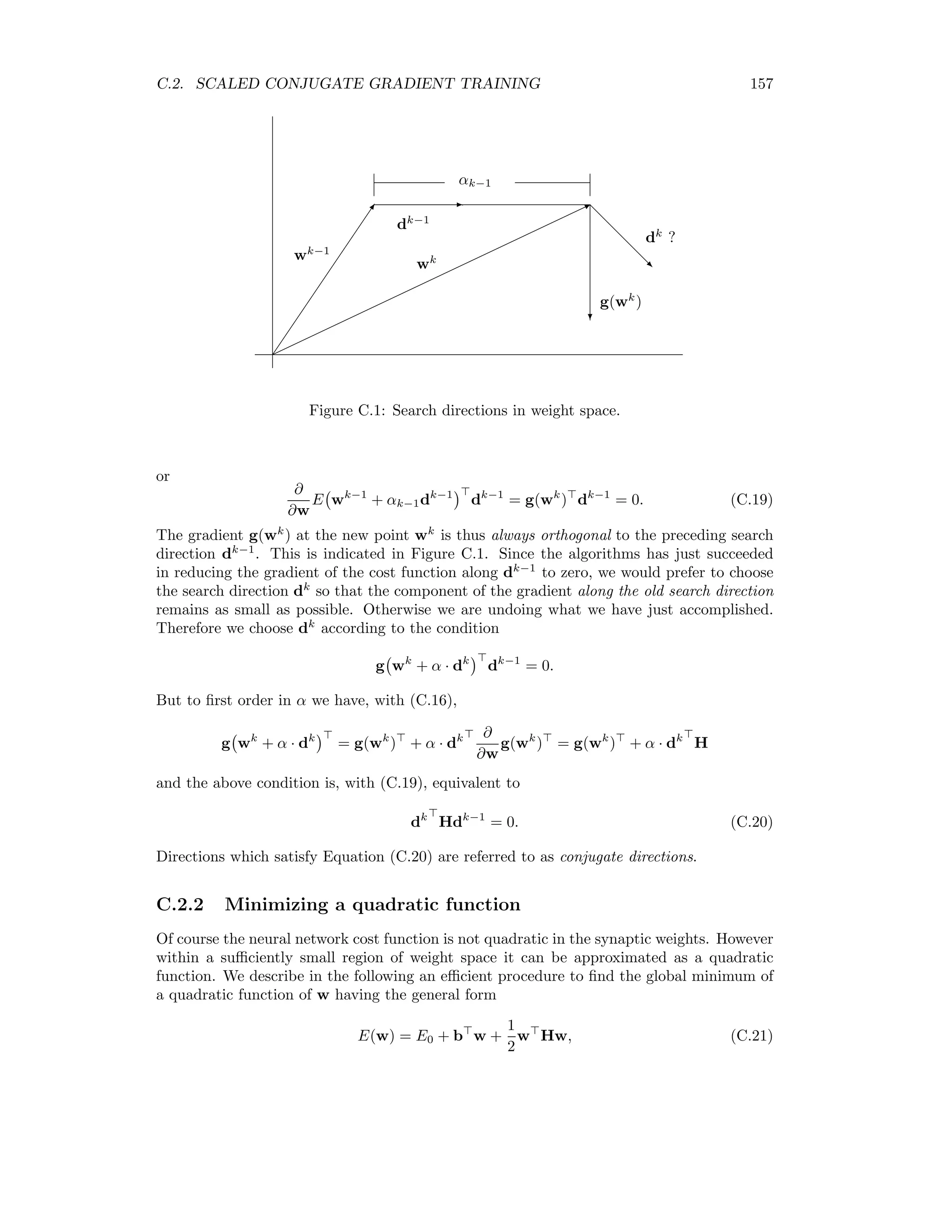
![152 APPENDIX C. ADVANCED NEURAL NETWORK TRAINING ALGORITHMS But then we have v Hv = v i βiλiui = i β2 i λi, and we conclude that H is positive definite if and only of all of its eigenvalues λi are positive. Thus a good way to check if one is at or near a local minimum in the cost function is to examine the eigenvalues of the Hessian. The scaled conjugate gradient algorithm makes explicit use of the Hessian matrix for more efficient convergence to a minimum in the cost function. The disadvantage of using H is that it is difficult to compute efficiently. For example, for a typical classification problem with N = 3-dimensional input data, L = 8 hidden neurons and M = 12 land use categories, there are [L(N + 1) + M(L + 1)]2 = 19, 600 matrix elements to determine at each iteration. We develop in the following an efficient method to calculate not H directly, but rather the product v H for any vector v having nw components. Our approach follows Bishop [Bis95] closely. C.1.1 The R-operator Let us begin by summarizing some results of Chapter 10 for the two-layer, feed forward network: x = (x1 . . . xN ) input observation y = (0 . . . 1 . . . 0) class label x = (1, x ) biased input observation Ih = Wh x activation vector for the hidden layer n = gh (Ih ) output signal vector from the hidden layer n = (1, n ) ditto with bias Io = Wo n activation vector for the output layer m = go (Io ) output vector from the network. (C.2) The corresponding activation functions are, for the hidden neurons, gh (Ih j ) = 1 1 + e−Ih j , j = 1 . . . L, (C.3) and for the output neurons, go (Io k) = eIo k M k =1 eIo k , k = 1 . . . M. (C.4) The first derivatives of the local cost function with respect to the output and hidden weights, (10.19) and (10.22), can be written concisely as ∂E ∂Wo = −nδo ∂E ∂Wh = −xδh , (C.5) where δo = y − m (C.6)](https://image.slidesharecdn.com/mortonjohncanty-imageanalysisandpatternrecognitionforremotesensingwithalgorithmsinenvi-idl-190425063306/75/Morton-john-canty-image-analysis-and-pattern-recognition-for-remote-sensing-with-algorithms-in-envi-idl-167-2048.jpg)
![C.1. THE HESSIAN MATRIX 153 and 0 δh = n ⊗ (1 − n) ⊗ Wo δo . (C.7) With Bishop [Bis95] we introduce the R-operator according to Rv{·} := v ∂ ∂w , v = (v1 . . . vnw ). Obviously we have Rv{w} = j vj ∂w ∂wj = v. We adopt the convention that the result of applying the R-operator has the same structure as the argument to which it is applied. Thus for example Rv{Wh } = Vh , where Vh , like Wh , is an (N + 1) × L matrix consisting of the first (N + 1) × L components of the vector v. Next we derive an expression for v H in terms of the R-operator. (v H)j = nw i=1 viHij = nw i=1 vi ∂2 E ∂wi∂wj = nw i=1 vi ∂ ∂wi ∂E ∂wj or (v H)j = v ∂ ∂w ∂E ∂wj = Rv ∂E ∂wj , j = 1 . . . nw. Since v H is a row vector, this can be written v H = Rv ∂E ∂w ∼= Rv ∂E ∂Wh , Rv ∂E ∂Wo . (C.8) Note the reorganization of the structure in the argument of Rv, namely w → (Wh , Wo ). This is merely for convenience. Once the expressions on the right have been evaluated, the result must be “flattened” back to a row vector. Equation (C.1.1) is understood to involve the local cost function. In order to complete the calculation we must sum over all training pairs. Applying the chain rule to (C.5), Rv ∂E ∂Wo = −nRv{δo } − RV {n}δo Rv ∂E ∂Wh = −xRv{δh }, (C.9) so that, in order to evaluate (C.1.1), we only need expressions for Rv{n}, Rv{δo } and Rv{δh }.](https://image.slidesharecdn.com/mortonjohncanty-imageanalysisandpatternrecognitionforremotesensingwithalgorithmsinenvi-idl-190425063306/75/Morton-john-canty-image-analysis-and-pattern-recognition-for-remote-sensing-with-algorithms-in-envi-idl-168-2048.jpg)
![C.1. THE HESSIAN MATRIX 155 C.1.2 Calculating the Hessian To calculate the Hessian matrix for the neural network, we evaluate (C.1.1) successively for the vectors v1 = (1, 0, 0 . . . 0) . . . vnw = (0, 0, 0 . . . 1) and build up H row for row: H = v1 H ... vnw H . The following excerpt from the IDL program FFNCG DEFINE (see Appendix D) imple- ments a vectorized version of the preceding calculation of v H and H: Function FFNCG::Rop, V nw = self.LL*(self.NN+1)+self.MM*(self.LL+1) ; reform V to dimensions of Wh and Wo and transpose VhT = transpose(reform(V[0:self.LL*(self.NN+1)-1],self.LL,self.NN+1)) Vo = reform(V[self.LL*(self.NN+1):*],self.MM,self.LL+1) VoT = transpose(Vo) ; transpose the weights WhT = transpose(*self.Wh) Wo = *self.Wo WoT = transpose(Wo) ; vectorized forward pass X = *self.Xs Zeroes = fltarr(self.p) Ones = Zeroes + 1.0 N = [[Ones],[1/(1+exp(-WhT##X))]] Io = WoT##N maxIo = max(Io,dimension=2) for k=0,self.MM-1 do Io[*,k]=Io[*,k]-maxIo A = exp(Io) sum = total(A,2) M = fltarr(self.p,self.MM) for k=0,self.MM-1 do M[*,k] = A[*,k]/sum ; evaluation of v^T.H D_o = *self.Ys-M ; d^o RIh = VhT##X ; Rv{I^h} RN = N*(1-N)*[[Zeroes],[RIh]] ; Rv{n} RIo = WoT##RN + VoT##N ; Rv{I^o} Rd_o = -M*(1-M)*RIo ; Rv{d^o} Rd_h = N*(1-N)*((1-2*N)*[[Zeroes],[RIh]]*(Wo##D_o) + Vo##D_o + Wo##Rd_o) Rd_h = Rd_h[*,1:*] ; Rv{d^h} REo = -N##transpose(Rd_o)-RN##transpose(D_o) ; Rv{dE/dWo} REh = -X##transpose(Rd_h) ; Rv{dE/dWh} return, [REh[*],REo[*]] ; v^T.H End](https://image.slidesharecdn.com/mortonjohncanty-imageanalysisandpatternrecognitionforremotesensingwithalgorithmsinenvi-idl-190425063306/75/Morton-john-canty-image-analysis-and-pattern-recognition-for-remote-sensing-with-algorithms-in-envi-idl-170-2048.jpg)
![156 APPENDIX C. ADVANCED NEURAL NETWORK TRAINING ALGORITHMS Function FFNCG::Hessian nw = self.LL*(self.NN+1)+self.MM*(self.LL+1) v = diag_matrix(fltarr(nw)+1.0) H = fltarr(nw,nw) for i=0,nw-1 do H[*,i] = self - Rop(v[*,i]) return, H End C.2 Scaled conjugate gradient training The backpropagation algorithm of Chapter 10 attempts to minimize the cost function locally, that is, weight updates are made immediately after presentation of a single training pair to the network. We will now consider a global approach aimed at minimization of the full cost function (10.15), which we denote in the following E(w). The symbol w is, as before, the nw-component vector of synaptic weights. Now let the gradient of the cost function at the point w be g(w), i.e. g(w) i = ∂ ∂wi E(w), i = 1 . . . nw. The Hessian matrix (H)ij = ∂2 E(w) ∂wi∂wj i, j = 1 . . . nw can then be expressed conveniently as the outer product H = ∂ ∂w g(w) . (C.16) C.2.1 Conjugate directions The search for a minimum in the cost function can be visualized as a series of points in the space of synaptic weight parameters, w1 , w2 . . . wk−1 , wk , wk+1 . . . , whereby the point wk is determined by minimizing E(w) along some search direction dk−1 which originated at the preceding point wk−1 . This is illustrated in Figure C.1 and corre- sponds to the vector equation wk = wk−1 + αk−1dk−1 . (C.17) Here dk−1 is a unit vector along the chosen search direction and the scalar αk−1 minimizes the cost function along that direction: αk−1 = arg min α E wk−1 + α · dk−1 . (C.18) If, starting from wk , we now wish to take the next minimizing step in the weight space, it is not efficient simply to choose, as in backpropagation, the direction of the local gradient g(wk) at the new starting point wk . It follows namely from (C.18) that ∂ ∂α E wk−1 + α · dk−1 α=αk−1 = 0](https://image.slidesharecdn.com/mortonjohncanty-imageanalysisandpatternrecognitionforremotesensingwithalgorithmsinenvi-idl-190425063306/75/Morton-john-canty-image-analysis-and-pattern-recognition-for-remote-sensing-with-algorithms-in-envi-idl-171-2048.jpg)
![158 APPENDIX C. ADVANCED NEURAL NETWORK TRAINING ALGORITHMS where b and H are constant and the matrix H is positive definite. The local gradient at the point w is given by g(w) = ∂ ∂w E(w) = b + Hw, and at the global minimum w∗ , b + Hw∗ = 0. (C.22) Now let {dk | k = 1 . . . nw} be a set of conjugate directions satisfying (C.20),1 dk Hd = 0 for k = , k, = 1 . . . nw. (C.23) The search directions dk are linearly independent. In order to demonstrate this let us assume the contrary, that is, that there exists an index k and constants αk , k = k, not all of which are zero, such that dk = nw k =1 k =k αk dk . But from (C.23) we have at once αk dk Hdk = 0 for k = k and, since H is positive definite, αk = 0 for k = k. The assumption thus leads to a contradiction and the dk are indeed linearly independent. The conjugate directions thus constitute a (non-orthogonal) vector basis for the entire weight space. In the search for the global minimum suppose we begin at an arbitrary point w1 and express the vector w∗ − w1 spanning the distance to the global minimum as a linear com- bination of the basis vectors dk : w∗ − w1 = nw k=1 αkdk . (C.24) Further, define wk = w1 + k−1 =1 α d (C.25) and split (C.24) up into nw steps wk+1 = wk + αkdk , k = 1 . . . nw. (C.26) At the kth step the search starts at the point wk and proceeds a distance αk along the conjugate direction dk . After nw such steps the global minimum w∗ is reached, since from (C.24–C.26) it follows that w∗ = w1 + nw k=1 αkdk = wnw + αnw dnw = wnw+1 . 1It can be shown that such a set always exists, see e.g. [Bis95].](https://image.slidesharecdn.com/mortonjohncanty-imageanalysisandpatternrecognitionforremotesensingwithalgorithmsinenvi-idl-190425063306/75/Morton-john-canty-image-analysis-and-pattern-recognition-for-remote-sensing-with-algorithms-in-envi-idl-173-2048.jpg)
![C.2. SCALED CONJUGATE GRADIENT TRAINING 161 This quantity is precisely 1 for a strictly quadratic function like (C.21). Therefore we can use the following heuristic: For the k + 1st iteration if ∆k 3/4, λk+1 := λk/2 if ∆k 1/4, λk+1 := 4λk else, λk+1 := λk. In other words, if the local quadratic approximation looks good according to criterion (C.32), then the step size can be increased (λk+1 is reduced relative to λk). If this is not the case then the step size is decreased (λk+1 is made larger). All of which leads us finally to the following algorithm (see e.g. [Moe93]) Algorithm (Scaled Conjugate Gradient) 1. Initialize the synaptic weights w with random numbers, set k = 0, λ = 0.001 and d = −g = −∂E(w)/∂w. 2. Set δ = d Hd + λ|d|2 . If δ 0, set λ = 2(λ − δ/d2 ) and δ = −d Hd. Save the current cost function E1 = E(w). 3. Determine the step size α = −d g/δ and new synaptic weights w = w + αd. 4. Calculate the quadricity ∆ = −(E1 − E(w))/(α · d g). If ∆ 1/4, restore the old weights: w = w − α · d, set λ = 4λ, d = −g and go to 2. 5. Set k = k + 1. If ∆ 3/4 set λ = λ/2. 6. Determine the new local gradient g = ∂E(w)/∂w and the new search direction d = −g + βd, whereby, if k mod nw = 0 then β = g Hd/(d Hd) else β = 0. 7. If E(w) is small enough stop, else go to 2. A few remarks on this algorithm: • The integer k counts the total number of iterations. Whenever k mod nw = 0 exactly nw weight updates have been carried out and the minimum of a truly quadratic func- tion would have been reached. This is taken as a good stage at which to restart the search along the negative local gradient −g rather than continuing along the current conjugate direction d. One expects that approximation errors will gradually corrupt the determination of the conjugate directions and the “fresh start” is intended to counter this. • Whenever the quadricity condition is not filled, i.e. whenever ∆ 1/4, the last weight update is cancelled and the search again restarted along −g. • Since the Hessian only occurs in the forms d H, and g H, it can be determined efficiently with the R-operator method. Here is an excerpt from the object FFNCG class extending FFN, showing the training method which implements scaled conjugate gradient algorithm:](https://image.slidesharecdn.com/mortonjohncanty-imageanalysisandpatternrecognitionforremotesensingwithalgorithmsinenvi-idl-190425063306/75/Morton-john-canty-image-analysis-and-pattern-recognition-for-remote-sensing-with-algorithms-in-envi-idl-176-2048.jpg)
![162 APPENDIX C. ADVANCED NEURAL NETWORK TRAINING ALGORITHMS Pro FFNCG::Train w = [(*self.Wh)[*],(*self.Wo)[*]] nw = n_elements(w) g = self-gradient() d = -g ; search direction, row vector k = 0L lambda = 0.001 window,12,xsize=600,ysize=400,title=’FFN(scaled conjugate gradient)’ wset,12 progressbar = Obj_New(’progressbar’, Color=’blue’, Text=’0’,$ title=’Training: epoch number...’,xsize=250,ysize=20) progressbar-start eivminmax = ’?’ repeat begin if progressbar-CheckCancel() then begin print,’Training interrupted’ progressbar-Destroy return endif d2 = total(d*d) ; d^2 dTHd = total(self-Rop(d)*d) ; d^T.H.d delta = dTHd+lambda*d2 if delta lt 0 then begin lambda = 2*(lambda-delta/d2) delta = -dTHd endif E1 = self-cost() ; E(w) (*self.cost_array)[k] = E1 dTg = total(d*g) ; d^T.g alpha = -dTg/delta dw = alpha*d w = w+dw *self.Wh = reform(w[0:self.LL*(self.NN+1)-1],self.LL,self.NN+1) *self.Wo = reform(w[self.LL*(self.NN+1):*],self.MM,self.LL+1) E2 = self-cost() ; E(w+dw) Ddelta = -(E1-E2)/(alpha*dTg) ; quadricity if Ddelta lt 0.25 then begin w = w - dw ; undo change in the weights *self.Wh = reform(w[0:self.LL*(self.NN+1)-1],self.LL,self.NN+1) *self.Wo = reform(w[self.LL*(self.NN+1):*],self.MM,self.LL+1) lambda = 4*lambda ; decrease step size d = -g ; restart along gradient end else begin k++ if Ddelta gt 0.75 then lambda = lambda/2 g = self-gradient() if k mod nw eq 0 then begin beta = 0 eivs = self-eigenvalues() eivminmax = string(min(eivs)/max(eivs),format=’(F10.6)’)](https://image.slidesharecdn.com/mortonjohncanty-imageanalysisandpatternrecognitionforremotesensingwithalgorithmsinenvi-idl-190425063306/75/Morton-john-canty-image-analysis-and-pattern-recognition-for-remote-sensing-with-algorithms-in-envi-idl-177-2048.jpg)
![C.3. KALMAN FILTER TRAINING 163 end else beta = total(self-Rop(g)*d)/dTHd d = beta*d-g plot,*self.cost_array,xrange=[0,k100],color=0,background=’FFFFFF’XL,$ ytitle=’cross entropy’,xtitle= $ ’Epoch [’+textoidl(’min(lambda)/max(lambda)=’)+eivminmax+’]’ endelse progressbar-Update,k*100/self.iterations,text=strtrim(k,2) endrep until k gt self.iterations End C.3 Kalman filter training In this Section we apply the recursive least squares method described in Appendix A to train the feed forward neural network of Figure 10.4. The appropriate cost function is the quadratic function (10.13) or, more specifically, its local version (10.14). 1 j L k ... ... ~q X b E 0 m( + 1) wo k 1 n1( + 1) nj( + 1) nL( + 1) n( + 1) Figure C.2: An isolated output neuron. We begin with consideration of the training process of an isolated neuron. Figure C.2 depicts an output neuron in the network during presentation of the + 1st training pair (x( + 1), y( + 1)). The neuron receives its input from the hidden layer (input vector n( + 1)) and generates the signal mk( + 1) = g(wo k n( + 1)) = ewo k n( +1) M k =1 ewo k n( +1 , k = 1 . . . M, which is compared to the desired output y( +1). It is easy to show that differentiation with respect to wo k yields ∂ ∂wo k g(wo k n( + 1)) = mk( + 1)(1 − mk( + 1))n( + 1). (C.33) and with respect to n, ∂ ∂n g(wo k n( + 1)) = mk( + 1)(1 − mk( + 1))wo k( + 1). (C.34)](https://image.slidesharecdn.com/mortonjohncanty-imageanalysisandpatternrecognitionforremotesensingwithalgorithmsinenvi-idl-190425063306/75/Morton-john-canty-image-analysis-and-pattern-recognition-for-remote-sensing-with-algorithms-in-envi-idl-178-2048.jpg)
![164 APPENDIX C. ADVANCED NEURAL NETWORK TRAINING ALGORITHMS C.3.1 Linearization We shall drop for the time being the indices on wo k, writing it simply as w. Let us call w( ) an approximation to the desired synaptic weight vector for our isolated output neuron, one which has been achieved so far in the training process, i.e. after presentation of the first training pairs. Then a linear approximation to mk( + 1) can be obtained by expanding in a first order Taylor series about the point w( ), m( + 1) ≈ g(w( ) n( + 1)) + ∂ ∂w g(w( ) n( + 1)) (w − w( )). With (C.34) we can then write m( + 1) ≈ ˆm( + 1) + ˆm( + 1)(1 − ˆm( + 1))n( + 1) (w − w( )), (C.35) where ˆm( + 1) is given by ˆm( + 1) = g(w( ) n( + 1)). With the definition of the linearized input A( + 1) = ˆm( + 1)(1 − ˆm( + 1))n( + 1) (C.36) we can write (C.35) in the form m( + 1) ≈ A( + 1)w + [ ˆm( + 1) − A( + 1)w( )]. The term in square brackets is - to first order - the error that arises from the fact that the neuron’s output signal is not simply proportional to w. If we neglect it altogether, then we get the linearized neuron output signal m( + 1) = A( )w. In order to calculate the synaptic weight vector w, we can now apply the theory of recursive least squares developed in Appendix A. We simply identify the parameter vector a with the synaptic weight vector w. We then have the least squares problem y y( + 1) = A A( + 1) w + . The Kalman filter equations for the recursive solution of this problem, Eq. (A.15), are unchanged: Σ +1 = I − K +1A( + 1) Σ K +1 = Σ A( + 1) A( + 1)Σ A( + 1) + 1 −1 . (C.37) while the recursive expression (A.14) for the parameter vector becomes w( + 1) = w( ) + K +1 y( + 1) − A( + 1)w( ) .](https://image.slidesharecdn.com/mortonjohncanty-imageanalysisandpatternrecognitionforremotesensingwithalgorithmsinenvi-idl-190425063306/75/Morton-john-canty-image-analysis-and-pattern-recognition-for-remote-sensing-with-algorithms-in-envi-idl-179-2048.jpg)

![C.3. KALMAN FILTER TRAINING 167 Algorithm (Kalman filter training) 1. Set = 0, Σh j (0) = 100 · Io , j = 1 . . . L, Σo k(0) = 100 · Ih , k = 1 . . . M and initialize the synaptic weight matrices Wh (0) and Wo (0) with random numbers. 2. Choose a training pair (x( +1), y( +1)) and determine the hidden layer output vector ˆn( + 1) = 1 g Wh ( ) x( + 1) and with it the quantities Ah j ( + 1) = ˆnj( + 1)(1 − ˆnj( + 1))x( + 1) , j = 1 . . . L, ˆmk( + 1) = g wo k ( )ˆn( + 1) Ao k( + 1) = ˆmk( + 1)(1 − ˆmk( + 1))ˆn( + 1) , k = 1 . . . M and βo ( + 1) = (y( + 1) − ˆm( + 1)) ⊗ ˆm( + 1) ⊗ (1 − ˆm( + 1)). 3. Determine the Kalman gains for all of the neurons according to Ko k( + 1) = Σo k( )Ao k( + 1) Ao k( + 1)Σo k( )Ao k( + 1) + 1 −1 , k = 1 . . . M Kh k( + 1) = Σh j ( )Ah j ( + 1) Ah j ( + 1)Σh j ( )Ah j ( + 1) + 1 −1 , j = 1 . . . L 4. Update the synaptic weight matrices: wo k( + 1) = wo k( ) + Ko k( + 1)[yk( + 1) − ˆmk( + 1)], k = 1 . . . M wh j ( + 1) = wh j ( ) + Kh j ( + 1) Wo j·( + 1)βo ( + 1) , j = 1 . . . L 5. Determine the new covariance matrices: Σo k( + 1) = Io − Ko k( + 1)Ao k( + 1) Σo k( ), k = 1 . . . M Σh j ( + 1) = Ih − Kh j ( + 1)Ah j ( + 1) Σh j ( ), j = 1 . . . L 6. If the overall cost function (10.13) is sufficiently small, stop, else set = + 1 and go to 2. This method was originally suggested by Shah and Palmieri [SP90], who called it the mul- tiple extended Kalman algorithm (MEKA). Here is an excerpt from the object FFNKAL class extending FFN, showing the class method which implements the Kalman filter algorithm: Pro FFNKAL:: train ; define update matrices for Wh and Wo dWh = fltarr(self.LL,self.NN+1) dWo = fltarr(self.MM,self.LL+1) iter = 0L iter100 = 0L progressbar = Obj_New(’progressbar’, Color=’blue’, Text=’0’,$ title=’Training: exemplar number...’,xsize=250,ysize=20)](https://image.slidesharecdn.com/mortonjohncanty-imageanalysisandpatternrecognitionforremotesensingwithalgorithmsinenvi-idl-190425063306/75/Morton-john-canty-image-analysis-and-pattern-recognition-for-remote-sensing-with-algorithms-in-envi-idl-182-2048.jpg)
![168 APPENDIX C. ADVANCED NEURAL NETWORK TRAINING ALGORITHMS progressbar-start window,12,xsize=600,ysize=400,title=’FFF(Kalman filter)’ wset,12 repeat begin if progressbar-CheckCancel() then begin print,’Training interrupted’ progressbar-Destroy return endif ; select exemplar pair at random ell = long(self.p*randomu(seed)) x=(*self.Xs)[ell,*] y=(*self.Ys)[ell,*] ; send it through the network m=self-forwardPass(x) ; error at output e=y-m ; loop over the output neurons for k=0,self.MM-1 do begin ; linearized input (column vector) Ao = m[k]*(1-m[k])*(*self.N) ; Kalman gain So = (*self.So)[*,*,k] SA = So##Ao Ko = SA/((transpose(Ao)##SA)[0]+1) ; determine delta for this neuron dWo[k,*] = Ko*e[k] ; update its covariance matrix So = So - Ko##transpose(Ao)##So (*self.So)[*,*,k] = So endfor ; update the output weights *self.Wo = *self.Wo + dWo ; backpropagated error beta_o =e*m*(1-m) ; loop over the hidden neurons for j=0,self.LL-1 do begin ; linearized input (column vector) Ah = X*(*self.N)[j+1]*(1-(*self.N)[j+1]) ; Kalman gain Sh = (*self.Sh)[*,*,j] SA = Sh##Ah Kh = SA/((transpose(Ah)##SA)[0]+1) ; determine delta for this neuron dWh[j,*] = Kh*((*self.Wo)[*,j+1]##beta_o)[0] ; update its covariance matrix Sh = Sh - Kh##transpose(Ah)##Sh (*self.Sh)[*,*,j] = Sh endfor ; update the hidden weights](https://image.slidesharecdn.com/mortonjohncanty-imageanalysisandpatternrecognitionforremotesensingwithalgorithmsinenvi-idl-190425063306/75/Morton-john-canty-image-analysis-and-pattern-recognition-for-remote-sensing-with-algorithms-in-envi-idl-183-2048.jpg)
![C.3. KALMAN FILTER TRAINING 169 *self.Wh = *self.Wh + dWh ; record cost history if iter mod 100 eq 0 then begin (*self.cost_array)[iter100]=alog10(self-cost()) iter100 = iter100+1 progressbar-Update,iter*100/self.iterations,text=strtrim(iter,2) plot,*self.cost_array,xrange=[0,iter100],color=0,background=’FFFFFF’XL,$ xtitle=’Iterations/100)’,ytitle=’log(cross entropy)’ end iter=iter+1 endrep until iter eq self.iterations progressbar-Destroy End](https://image.slidesharecdn.com/mortonjohncanty-imageanalysisandpatternrecognitionforremotesensingwithalgorithmsinenvi-idl-190425063306/75/Morton-john-canty-image-analysis-and-pattern-recognition-for-remote-sensing-with-algorithms-in-envi-idl-184-2048.jpg)


![178 APPENDIX D. ENVI EXTENSIONS ; AUTHOR ; Mort Canty (2004) ; Juelich Research Center ; m.canty@fz-juelich.de ; CALLING SEQUENCE: ; dwt = Obj_New(DWT,image) ; ARGUMENTS: ; image: grayscale image to be compressed ; KEYWORDS ; None ; METHODS: ; SET_COEFF: choose the Daubechies wavelet ; dwt - Set_Coeff, n ; n = 4,6,8,12 ; SHOW_IMAGE: display the image pyramid in a window ; dwt - Show_Image, wn ; INJECT: overwrite upper left quadrant ; after phase correlation match if keyword pc is set (default) ; dwt - Inject, array, pc = pc ; SET_COMPRESSIONS: set the number of compressions ; dwt - Set_Compressions, nc ; GET_COMPRESSIONS: get the number of compressions ; nc = dwt - Get_Compressions() ; GET_NUM_COLS: get the number of columns in the compressed image ; cols = dwt - Get_Num_Cols() ; GET_NUM_ROWS: get the number of rows in the compressed image ; cols = dwt - Get_Num_Rows() ; GET_IMAGE: return the pyramid image ; im = dwt - Get_Image() ; GET_QUADRANT: get compressed image (as 2D array) or innermost ; wavelet coefficients as vector ; wc = dwt - Get_Quadrant(n) ; n = 0,1,2,3 ; NORMALIZE_WC: normalize wavelet coefficients at all levels ; dwt - Normalize, a, b ; a, b are normalization parameters ; COMPRESS: perform a single compression ; dwt - Compress ; dwt - Inject, array, pcr=pc ; EXPAND: perfrom a single expansion ; dwt - Expand ; DEPENDENCIES: ; PHASE_CORR ; --------------------------------------------------------------------- ;+ ; NAME: ; PHASE_CORR ; PURPOSE: ; Returns relative offset [xoff,yoff] of two images using phase correlation](https://image.slidesharecdn.com/mortonjohncanty-imageanalysisandpatternrecognitionforremotesensingwithalgorithmsinenvi-idl-190425063306/75/Morton-john-canty-image-analysis-and-pattern-recognition-for-remote-sensing-with-algorithms-in-envi-idl-193-2048.jpg)