Machine Learning with Python- Machine Learning Algorithms- Naïve Bayes.pdf

Machine Learning with Python- Machine Learning Algorithms- Naïve Bayes.pdf

• 1.
  Machine Learning withPython Machine Learning Algorithms - Naïve Bayes Prof.ShibdasDutta, Associate Professor, DCGDATACORESYSTEMSINDIAPVTLTD Kolkata Company Confidential: Data-Core Systems, Inc. | datacoresystems.com
• 2.
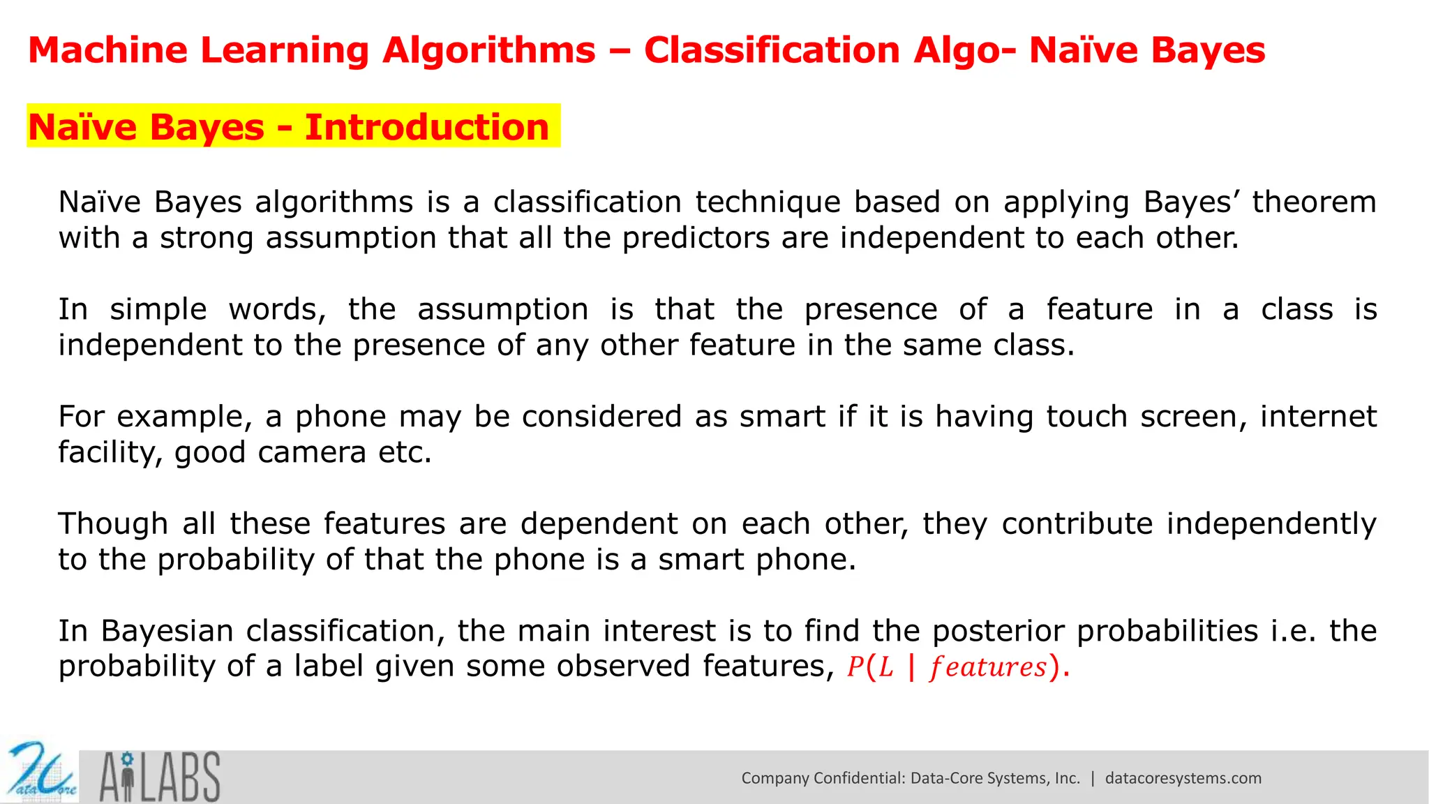
  Machine Learning Algorithms– Classification Algo- Naïve Bayes Naïve Bayes - Introduction Naïve Bayes algorithms is a classification technique based on applying Bayes’ theorem with a strong assumption that all the predictors are independent to each other. In simple words, the assumption is that the presence of a feature in a class is independent to the presence of any other feature in the same class. For example, a phone may be considered as smart if it is having touch screen, internet facility, good camera etc. Though all these features are dependent on each other, they contribute independently to the probability of that the phone is a smart phone. In Bayesian classification, the main interest is to find the posterior probabilities i.e. the probability of a label given some observed features, 𝑃(𝐿 | 𝑓𝑒𝑎𝑡𝑢𝑟𝑒𝑠). Company Confidential: Data-Core Systems, Inc. | datacoresystems.com
• 3.
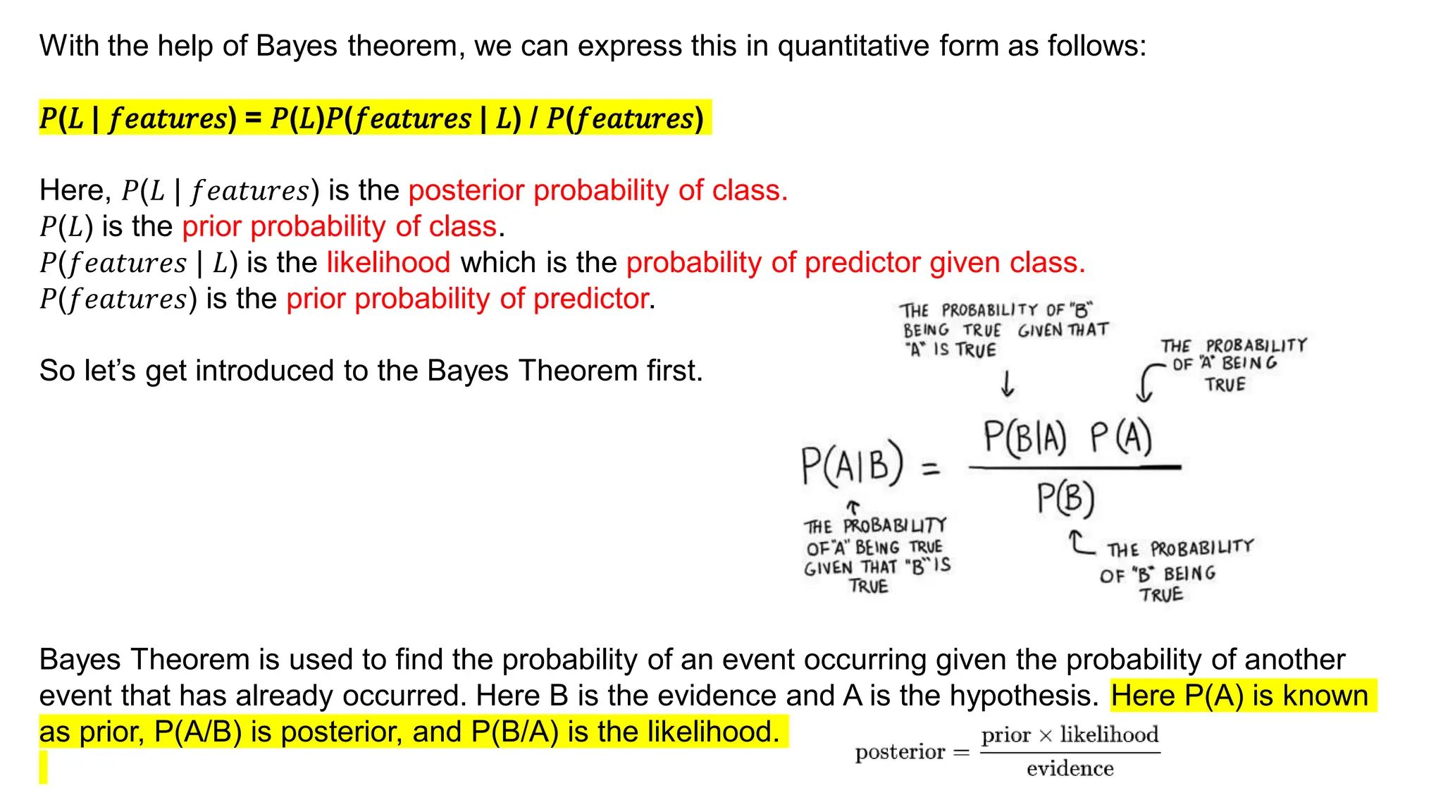
  With the helpof Bayes theorem, we can express this in quantitative form as follows: 𝑃(𝐿 | 𝑓𝑒𝑎𝑡𝑢𝑟𝑒𝑠) = 𝑃(𝐿)𝑃(𝑓𝑒𝑎𝑡𝑢𝑟𝑒𝑠 | 𝐿) / 𝑃(𝑓𝑒𝑎𝑡𝑢𝑟𝑒𝑠) Here, 𝑃(𝐿 | 𝑓𝑒𝑎𝑡𝑢𝑟𝑒𝑠) is the posterior probability of class. 𝑃(𝐿) is the prior probability of class. 𝑃(𝑓𝑒𝑎𝑡𝑢𝑟𝑒𝑠 | 𝐿) is the likelihood which is the probability of predictor given class. 𝑃(𝑓𝑒𝑎𝑡𝑢𝑟𝑒𝑠) is the prior probability of predictor. So let’s get introduced to the Bayes Theorem first. Bayes Theorem is used to find the probability of an event occurring given the probability of another event that has already occurred. Here B is the evidence and A is the hypothesis. Here P(A) is known as prior, P(A/B) is posterior, and P(B/A) is the likelihood.
• 4.
  The name Naiveis used because the presence of one independent feature doesn’t affect (influence or change the value of) other features. The most important assumption that Naive Bayes makes is that all the features are independent of each other. Being less prone to overfitting, Naive Bayes algorithm works on Bayes theorem to predict unknown data sets. Company Confidential: Data-Core Systems, Inc. | datacoresystems.com
• 5.
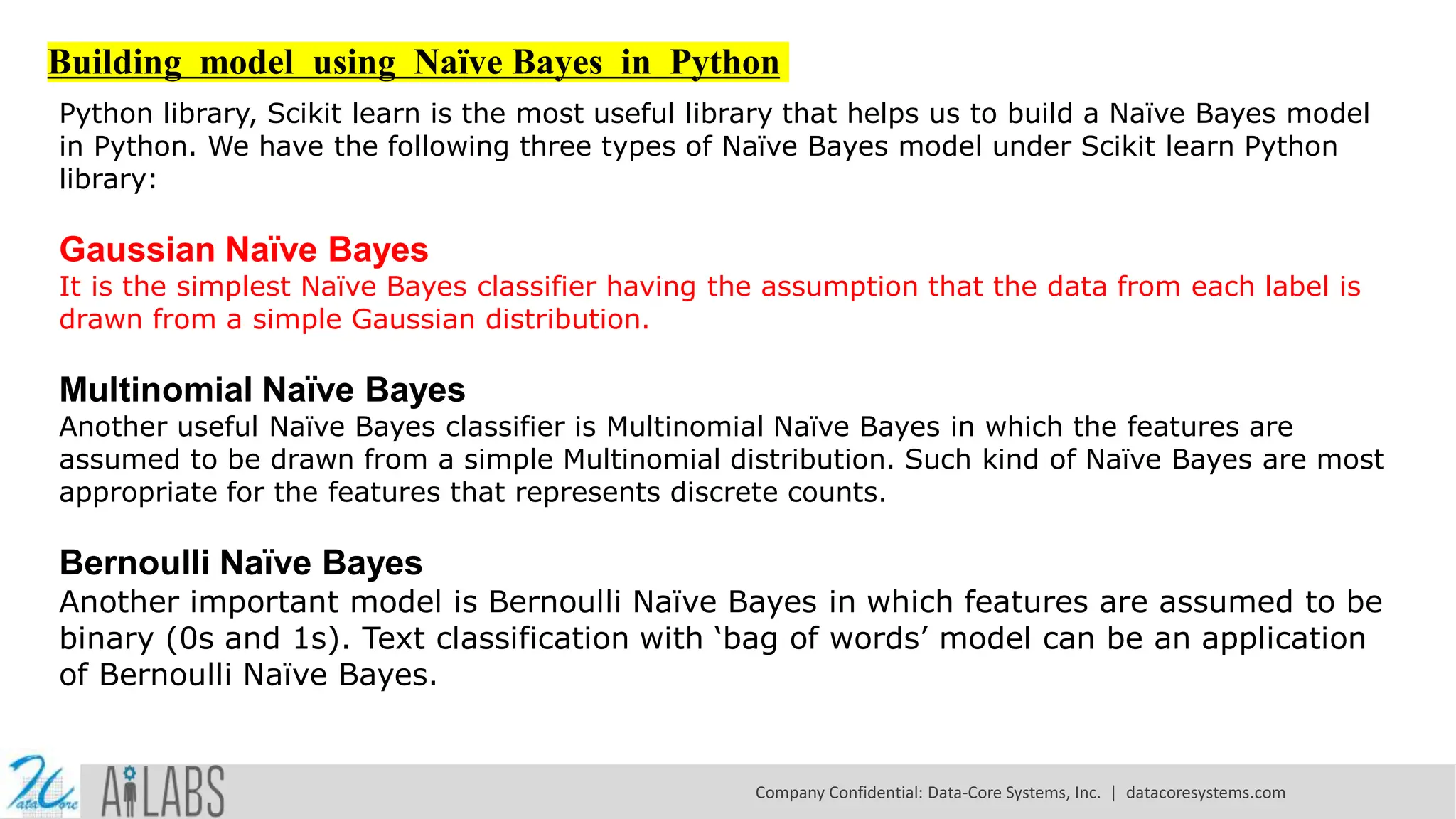
  Building model usingNaïve Bayes in Python Python library, Scikit learn is the most useful library that helps us to build a Naïve Bayes model in Python. We have the following three types of Naïve Bayes model under Scikit learn Python library: Gaussian Naïve Bayes It is the simplest Naïve Bayes classifier having the assumption that the data from each label is drawn from a simple Gaussian distribution. Multinomial Naïve Bayes Another useful Naïve Bayes classifier is Multinomial Naïve Bayes in which the features are assumed to be drawn from a simple Multinomial distribution. Such kind of Naïve Bayes are most appropriate for the features that represents discrete counts. Bernoulli Naïve Bayes Another important model is Bernoulli Naïve Bayes in which features are assumed to be binary (0s and 1s). Text classification with ‘bag of words’ model can be an application of Bernoulli Naïve Bayes. Company Confidential: Data-Core Systems, Inc. | datacoresystems.com
• 6.
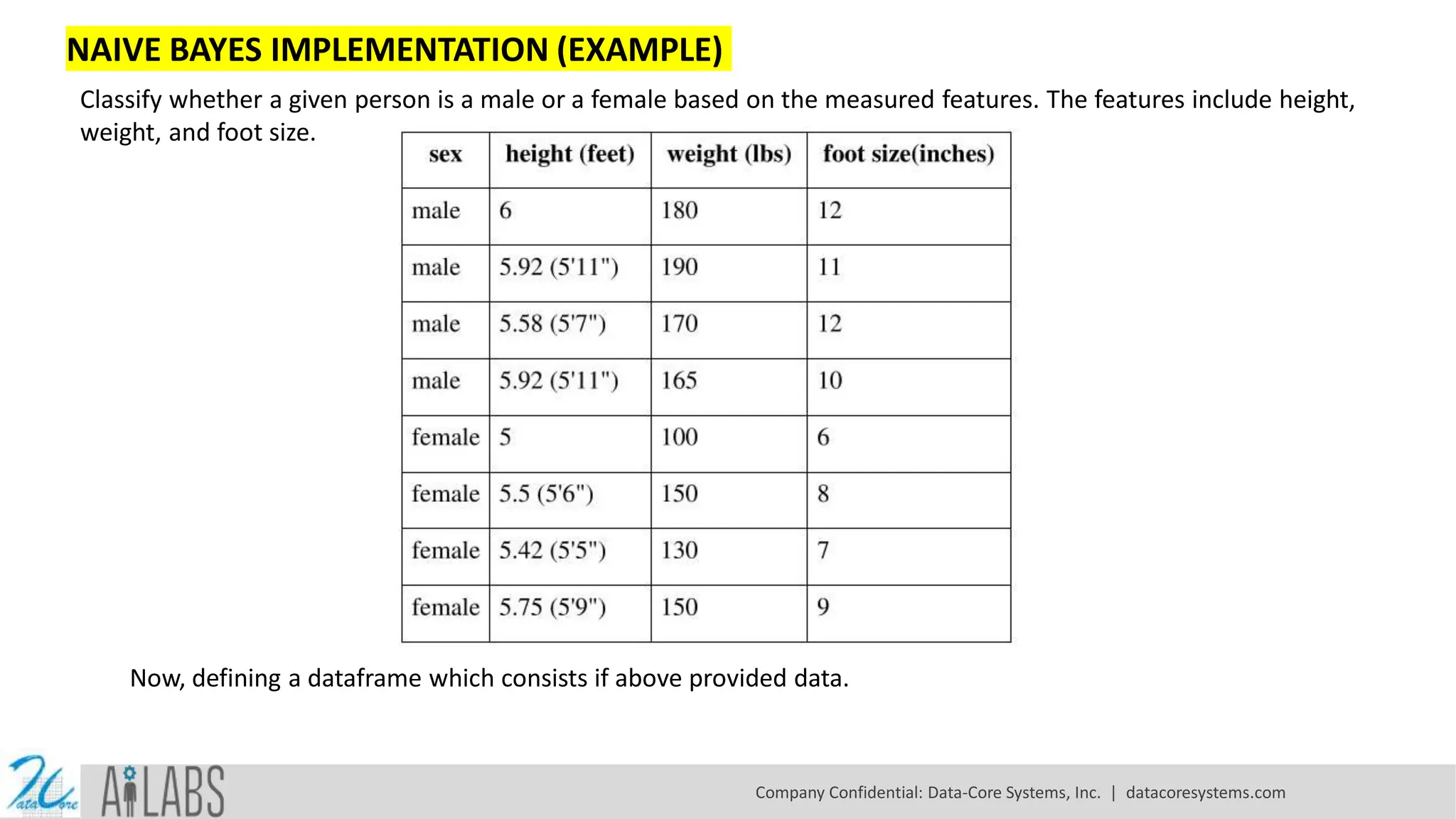
  NAIVE BAYES IMPLEMENTATION(EXAMPLE) Classify whether a given person is a male or a female based on the measured features. The features include height, weight, and foot size. Now, defining a dataframe which consists if above provided data. Company Confidential: Data-Core Systems, Inc. | datacoresystems.com
• 7.
  import pandas aspd import numpy as np # Create an empty dataframe data = pd.DataFrame() # Create our target variable data['Gender'] = ['male','male','male','male','female','female','female','female'] # Create our feature variables data['Height'] = [6,5.92,5.58,5.92,5,5.5,5.42,5.75] data['Weight'] = [180,190,170,165,100,150,130,150] data['Foot_Size'] = [12,11,12,10,6,8,7,9] Creating another data frame containing the feature value of height as 6 feet, weight as 130 lbs and foot size as 8 inches. using Naive Bayes , trying to find whether the gender is male or female. # Create an empty dataframe person = pd.DataFrame() # Create some feature values for this single row person['Height'] = [6] person['Weight'] = [130] person['Foot_Size'] = [8] Company Confidential: Data-Core Systems, Inc. | datacoresystems.com
• 8.
  Calculating the totalnumber of males and females and their probabilities i.e priors: # Number of males n_male = data['Gender'][data['Gender'] == 'male'].count() # Number of females n_female = data['Gender'][data['Gender'] == 'female'].count() # Total rows total_ppl = data['Gender'].count() # Number of males divided by the total rows P_male = n_male/total_ppl # Number of females divided by the total rows P_female = n_female/total_ppl Company Confidential: Data-Core Systems, Inc. | datacoresystems.com
• 9.
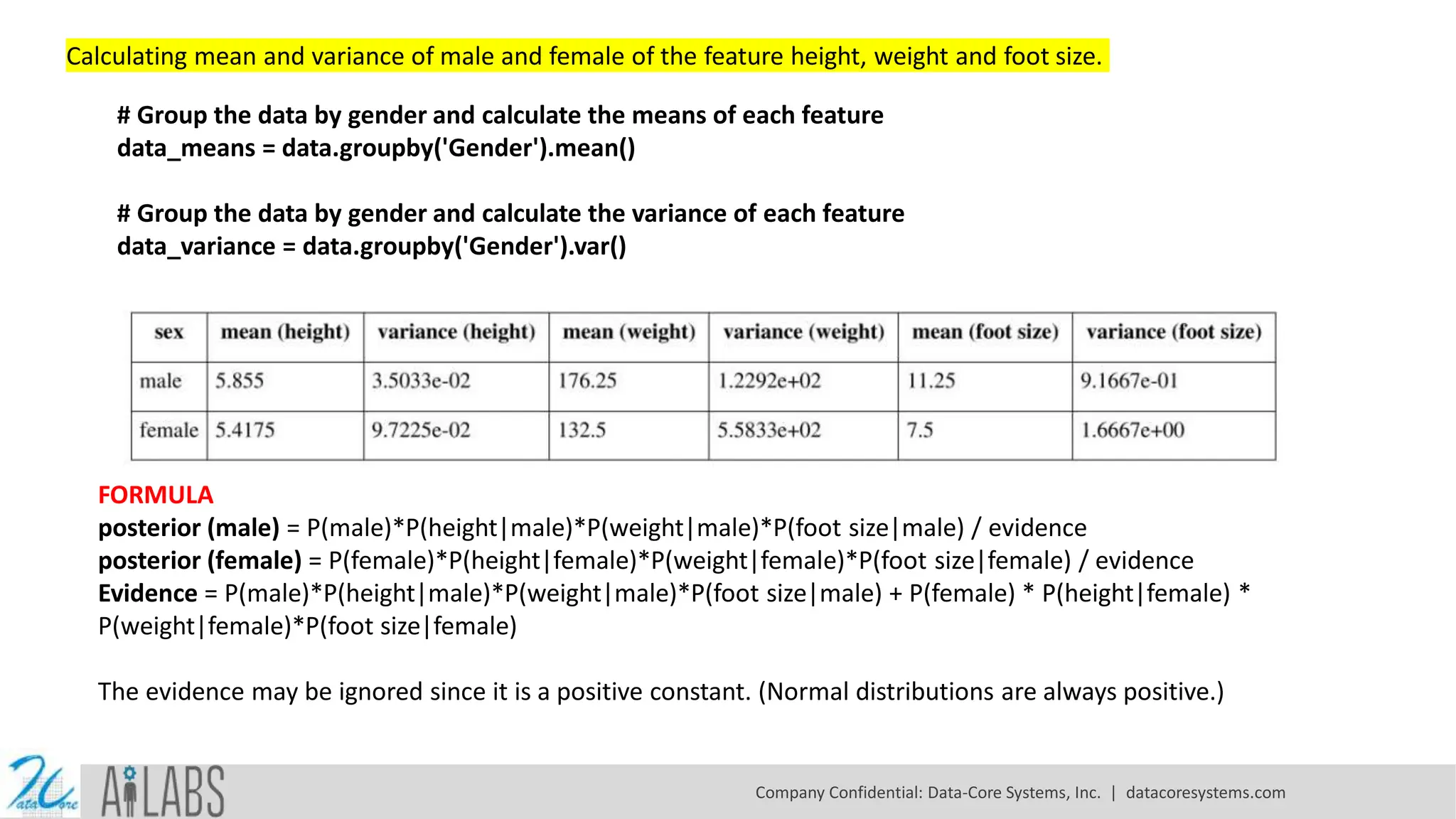
  Calculating mean andvariance of male and female of the feature height, weight and foot size. # Group the data by gender and calculate the means of each feature data_means = data.groupby('Gender').mean() # Group the data by gender and calculate the variance of each feature data_variance = data.groupby('Gender').var() FORMULA posterior (male) = P(male)*P(height|male)*P(weight|male)*P(foot size|male) / evidence posterior (female) = P(female)*P(height|female)*P(weight|female)*P(foot size|female) / evidence Evidence = P(male)*P(height|male)*P(weight|male)*P(foot size|male) + P(female) * P(height|female) * P(weight|female)*P(foot size|female) The evidence may be ignored since it is a positive constant. (Normal distributions are always positive.) Company Confidential: Data-Core Systems, Inc. | datacoresystems.com
• 10.
  CALCULATION Nominal distribution formula CompanyConfidential: Data-Core Systems, Inc. | datacoresystems.com
• 11.
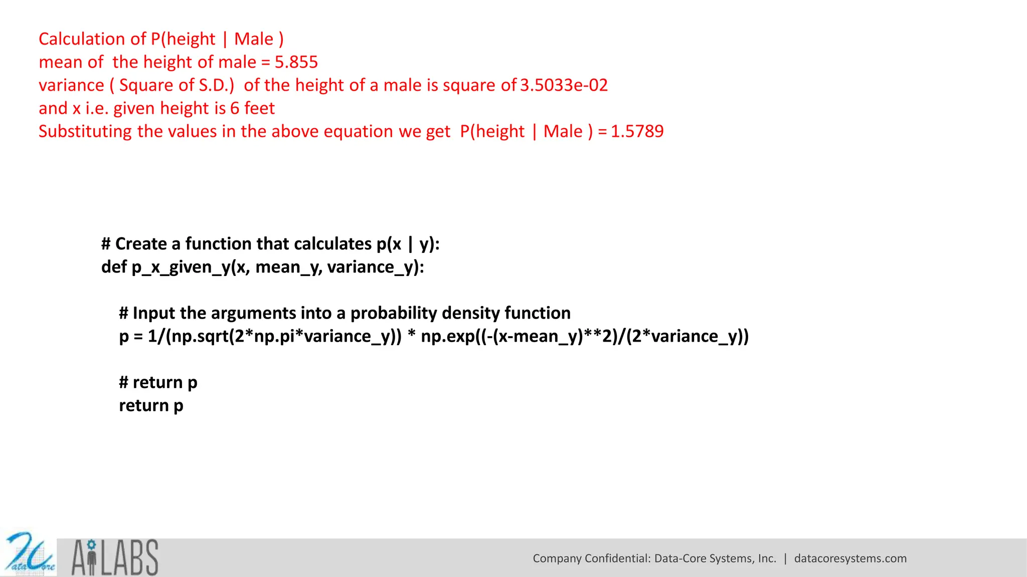
  Calculation of P(height| Male ) mean of the height of male = 5.855 variance ( Square of S.D.) of the height of a male is square of 3.5033e-02 and x i.e. given height is 6 feet Substituting the values in the above equation we get P(height | Male ) = 1.5789 # Create a function that calculates p(x | y): def p_x_given_y(x, mean_y, variance_y): # Input the arguments into a probability density function p = 1/(np.sqrt(2*np.pi*variance_y)) * np.exp((-(x-mean_y)**2)/(2*variance_y)) # return p return p Company Confidential: Data-Core Systems, Inc. | datacoresystems.com
• 12.
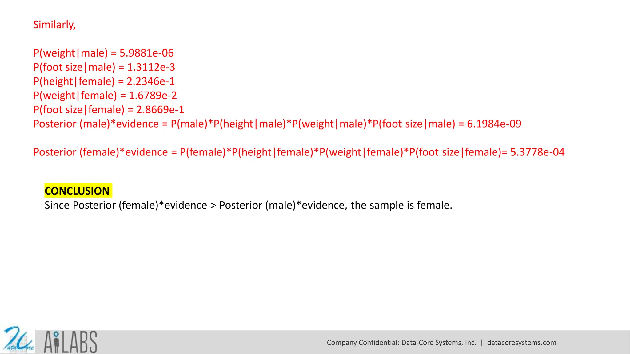
  Similarly, P(weight|male) = 5.9881e-06 P(footsize|male) = 1.3112e-3 P(height|female) = 2.2346e-1 P(weight|female) = 1.6789e-2 P(foot size|female) = 2.8669e-1 Posterior (male)*evidence = P(male)*P(height|male)*P(weight|male)*P(foot size|male) = 6.1984e-09 Posterior (female)*evidence = P(female)*P(height|female)*P(weight|female)*P(foot size|female)= 5.3778e-04 CONCLUSION Since Posterior (female)*evidence > Posterior (male)*evidence, the sample is female. Company Confidential: Data-Core Systems, Inc. | datacoresystems.com
• 13.
  NAIVE BAYES USINGSCIKIT-LEARN import pandas as pd import numpy as np # Create an empty dataframe data = pd.DataFrame() # Create our target variable data['Gender'] = [1,1,1,1,0,0,0,0] #1 is male # Create our feature variables data['Height'] = [6,5.92,5.58,5.92,5,5.5,5.42,5.75] data['Weight'] = [180,190,170,165,100,150,130,150] data['Foot_Size'] = [12,11,12,10,6,8,7,9] # View the data data Though we have very small dataset, we are dividing the dataset into train and test do that it can be used in other model prediction. We are importing gnb() from sklearn and we are training the model with out dataset. Company Confidential: Data-Core Systems, Inc. | datacoresystems.com
• 14.
  X = data.drop(['Gender'],axis=1) y=data.Gender #splitting X and y into training and testing sets from sklearn.model_selection import train_test_split X_train, X_test, y_train, y_test = train_test_split(X, y, test_size=0.4, random_state=1) # training the model on training set from sklearn.naive_bayes import GaussianNB gnb = GaussianNB() gnb.fit(X_train, y_train) # making predictions on the testing set y_pred = gnb.predict(X_test) Company Confidential: Data-Core Systems, Inc. | datacoresystems.com
• 15.
  from sklearn.metrics importclassification_report, confusion_matrix print(classification_report(y, gnb.predict(X))) cm = confusion_matrix(y, gnb.predict(X)) fig, ax = plt.subplots(figsize=(8, 8)) ax.imshow(cm) ax.grid(False) ax.xaxis.set(ticks=(0, 1), ticklabels=('Predicted 0s', 'Predicted 1s')) ax.yaxis.set(ticks=(0, 1), ticklabels=('Actual 0s', 'Actual 1s')) ax.set_ylim(1.5, -0.5) for i in range(2): for j in range(2): ax.text(j, i, cm[i, j], ha='center', va='center', color='red') plt.show() Company Confidential: Data-Core Systems, Inc. | datacoresystems.com
• 16.
  Now, our modelis ready. Let’s use this model to predict on new data. # Create our target variable data1 = pd.DataFrame() # Create our feature variables data1['Height'] = [6] data1['Weight'] = [130] data1['Foot_Size'] = [8] y_pred = gnb.predict(data1) if y_pred==0: print ("female") else: print ("male") Output: Female Company Confidential: Data-Core Systems, Inc. | datacoresystems.com
• 17.
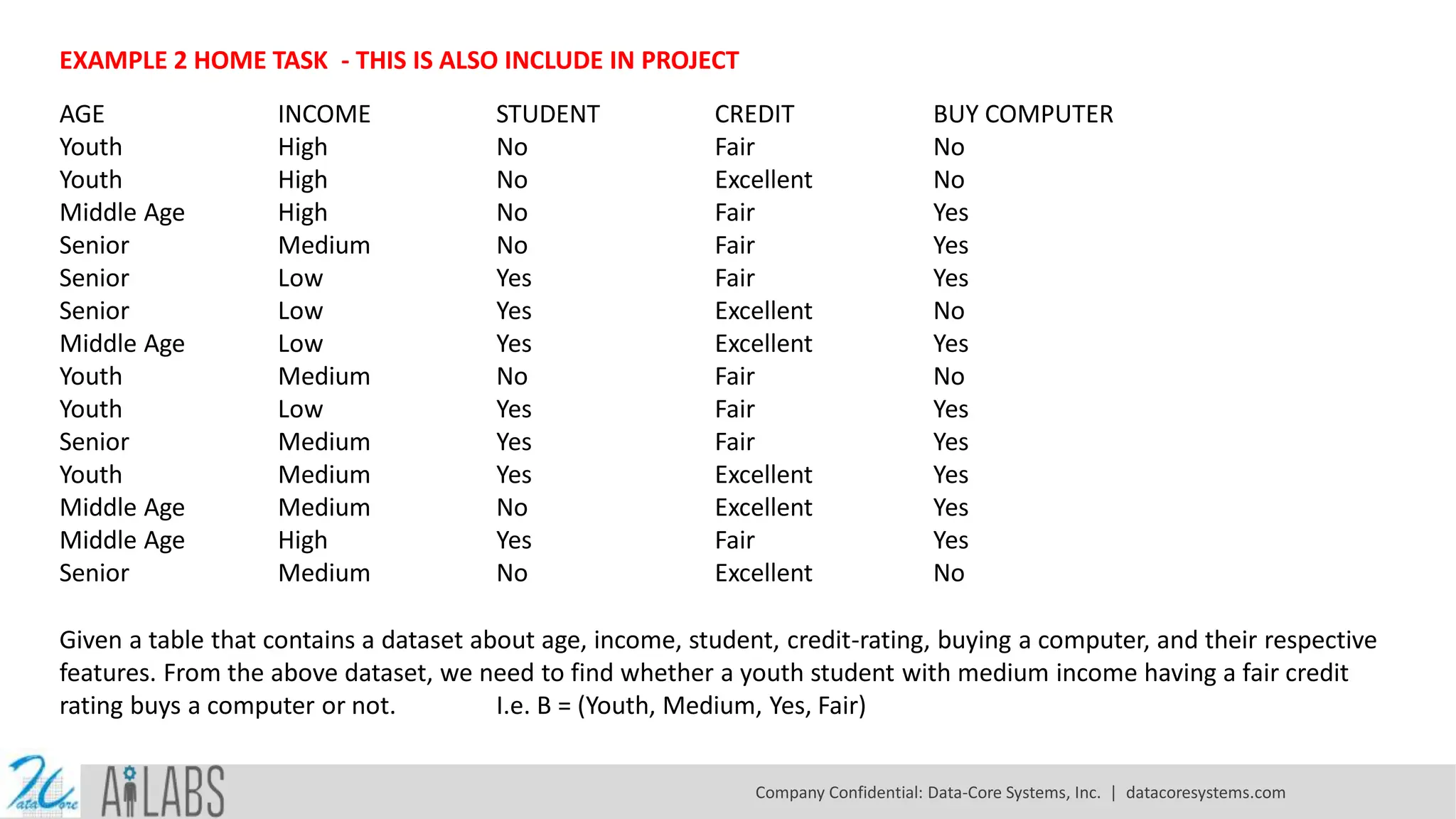
  EXAMPLE 2 HOMETASK - THIS IS ALSO INCLUDE IN PROJECT AGE INCOME STUDENT CREDIT BUY COMPUTER Youth High No Fair No Youth High No Excellent No Middle Age High No Fair Yes Senior Medium No Fair Yes Senior Low Yes Fair Yes Senior Low Yes Excellent No Middle Age Low Yes Excellent Yes Youth Medium No Fair No Youth Low Yes Fair Yes Senior Medium Yes Fair Yes Youth Medium Yes Excellent Yes Middle Age Medium No Excellent Yes Middle Age High Yes Fair Yes Senior Medium No Excellent No Given a table that contains a dataset about age, income, student, credit-rating, buying a computer, and their respective features. From the above dataset, we need to find whether a youth student with medium income having a fair credit rating buys a computer or not. I.e. B = (Youth, Medium, Yes, Fair) Company Confidential: Data-Core Systems, Inc. | datacoresystems.com
• 18.
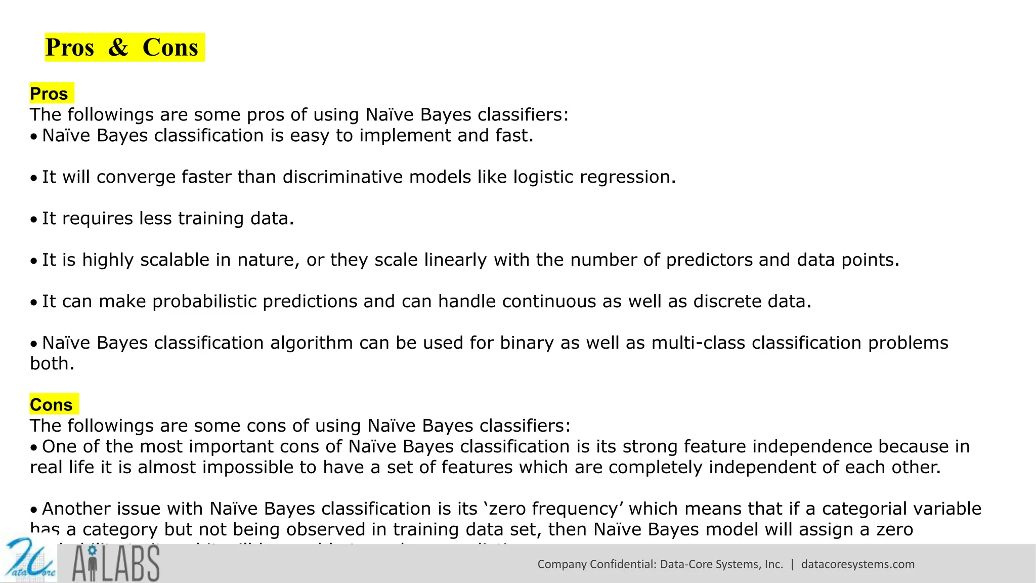
  Pros & Cons Pros Thefollowings are some pros of using Naïve Bayes classifiers: Naïve Bayes classification is easy to implement and fast. It will converge faster than discriminative models like logistic regression. It requires less training data. It is highly scalable in nature, or they scale linearly with the number of predictors and data points. It can make probabilistic predictions and can handle continuous as well as discrete data. Naïve Bayes classification algorithm can be used for binary as well as multi-class classification problems both. Cons The followings are some cons of using Naïve Bayes classifiers: One of the most important cons of Naïve Bayes classification is its strong feature independence because in real life it is almost impossible to have a set of features which are completely independent of each other. Another issue with Naïve Bayes classification is its ‘zero frequency’ which means that if a categorial variable has a category but not being observed in training data set, then Naïve Bayes model will assign a zero probability to it and it will be unable to make a prediction. Company Confidential: Data-Core Systems, Inc. | datacoresystems.com
• 19.
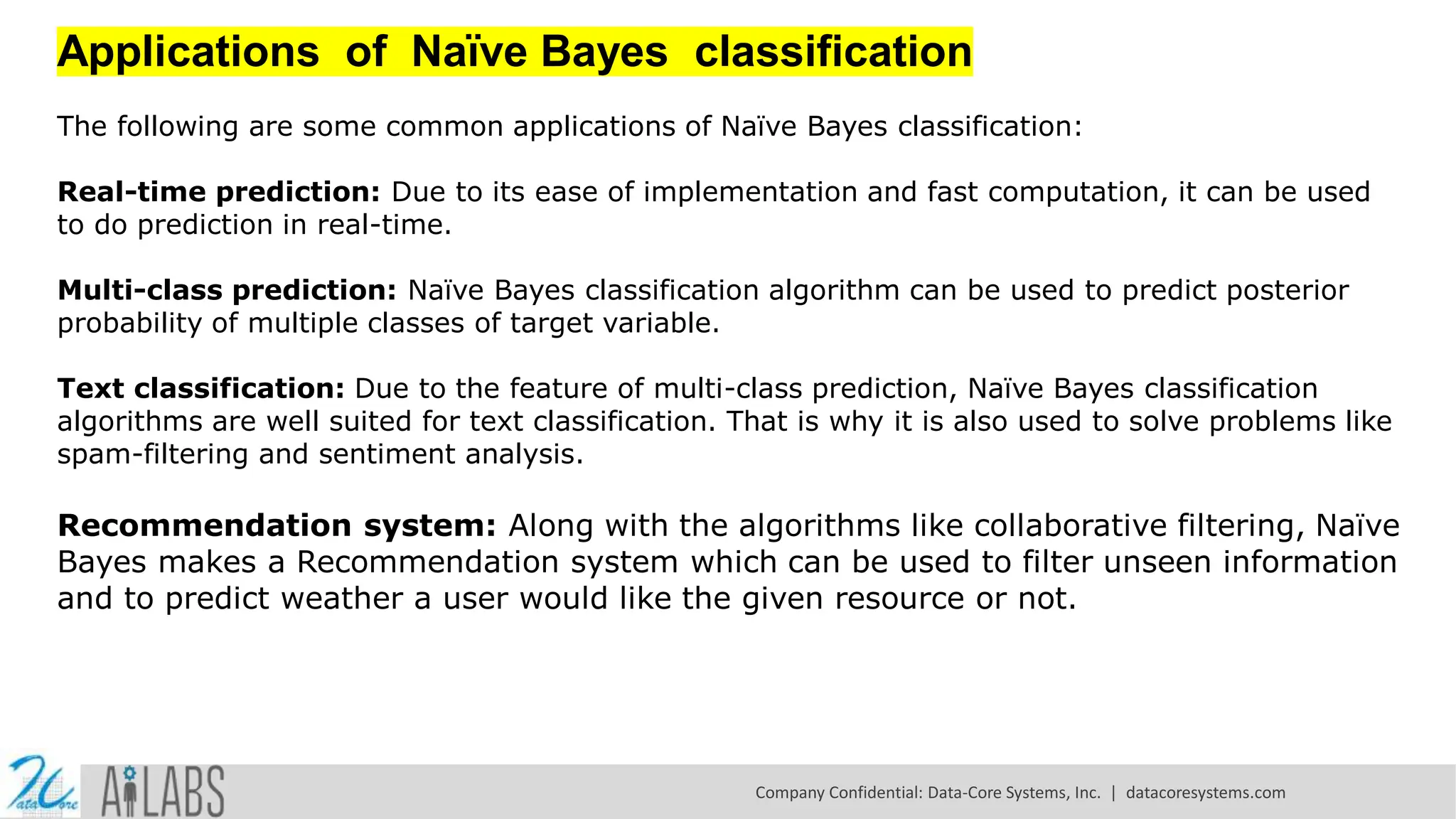
  Applications of NaïveBayes classification The following are some common applications of Naïve Bayes classification: Real-time prediction: Due to its ease of implementation and fast computation, it can be used to do prediction in real-time. Multi-class prediction: Naïve Bayes classification algorithm can be used to predict posterior probability of multiple classes of target variable. Text classification: Due to the feature of multi-class prediction, Naïve Bayes classification algorithms are well suited for text classification. That is why it is also used to solve problems like spam-filtering and sentiment analysis. Recommendation system: Along with the algorithms like collaborative filtering, Naïve Bayes makes a Recommendation system which can be used to filter unseen information and to predict weather a user would like the given resource or not. Company Confidential: Data-Core Systems, Inc. | datacoresystems.com
• 20.
  Thank You Company Confidential:Data-Core Systems, Inc. | datacoresystems.com