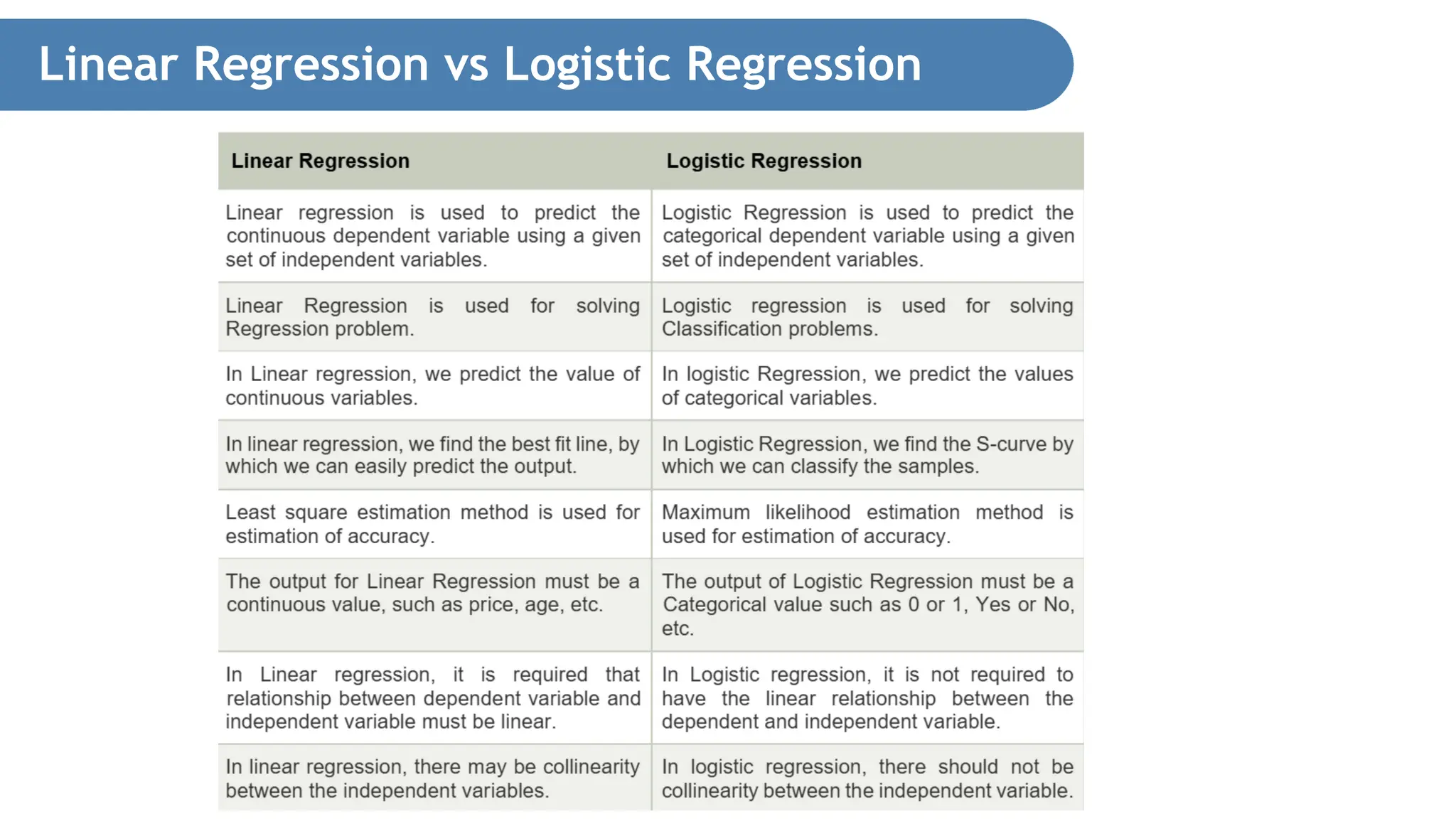
Logistic Regression in machine learning ppt

02/18/2025 • Logistic regression is one of the most popular Machine Learning algorithms, which comes under the Supervised Learning technique. • It is used for predicting the categorical dependent variable using a given set of independent variables. • The outcome must be a categorical or discrete value. It can be either Yes or No, 0 or 1, true or False, etc. but instead of giving the exact value as 0 and 1, it gives the probabilistic values which lie between 0 and 1. • Logistic Regression is much similar to the Linear Regression except that how they are used. Linear Regression is used for solving Regression problems, whereas Logistic regression is used for solving the classification problems. • In Logistic regression, instead of fitting a regression line, we fit an “S” shaped logistic function, which predicts two maximum values (0 or 1). Logistic Regression

02/18/2025 Types of Logistic Regression • Binomial: In binomial Logistic regression, there can be only two possible types of the dependent variables, such as 0 or 1, Pass or Fail, etc. • Multinomial: In multinomial Logistic regression, there can be 3 or more possible unordered types of the dependent variable, such as “cat”, “dogs”, or “sheep” • Ordinal: In ordinal Logistic regression, there can be 3 or more possible ordered types of dependent variables, such as “low”, “Medium”, or “High”. Logistic Regression

02/18/2025 Why do we use Logistic Regression rather than Linear Regression? • It is only used when our dependent variable is binary and in linear regression this dependent variable is continuous. • The second problem is that if we add an outlier in our dataset, the best fit line in linear regression shifts to fit that point. Logistic Regression

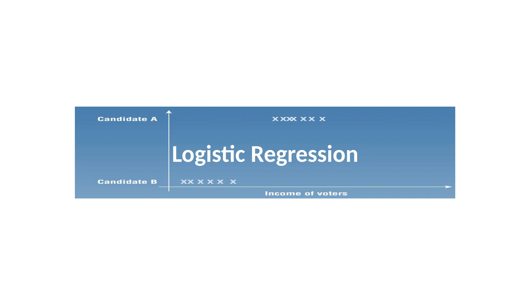
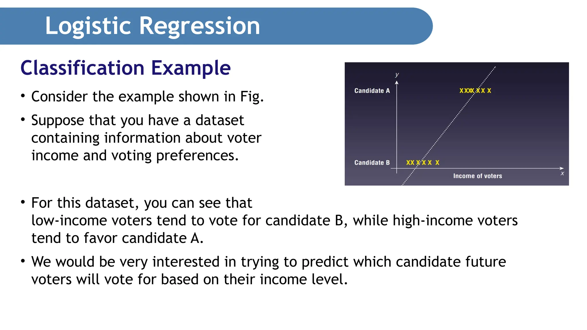
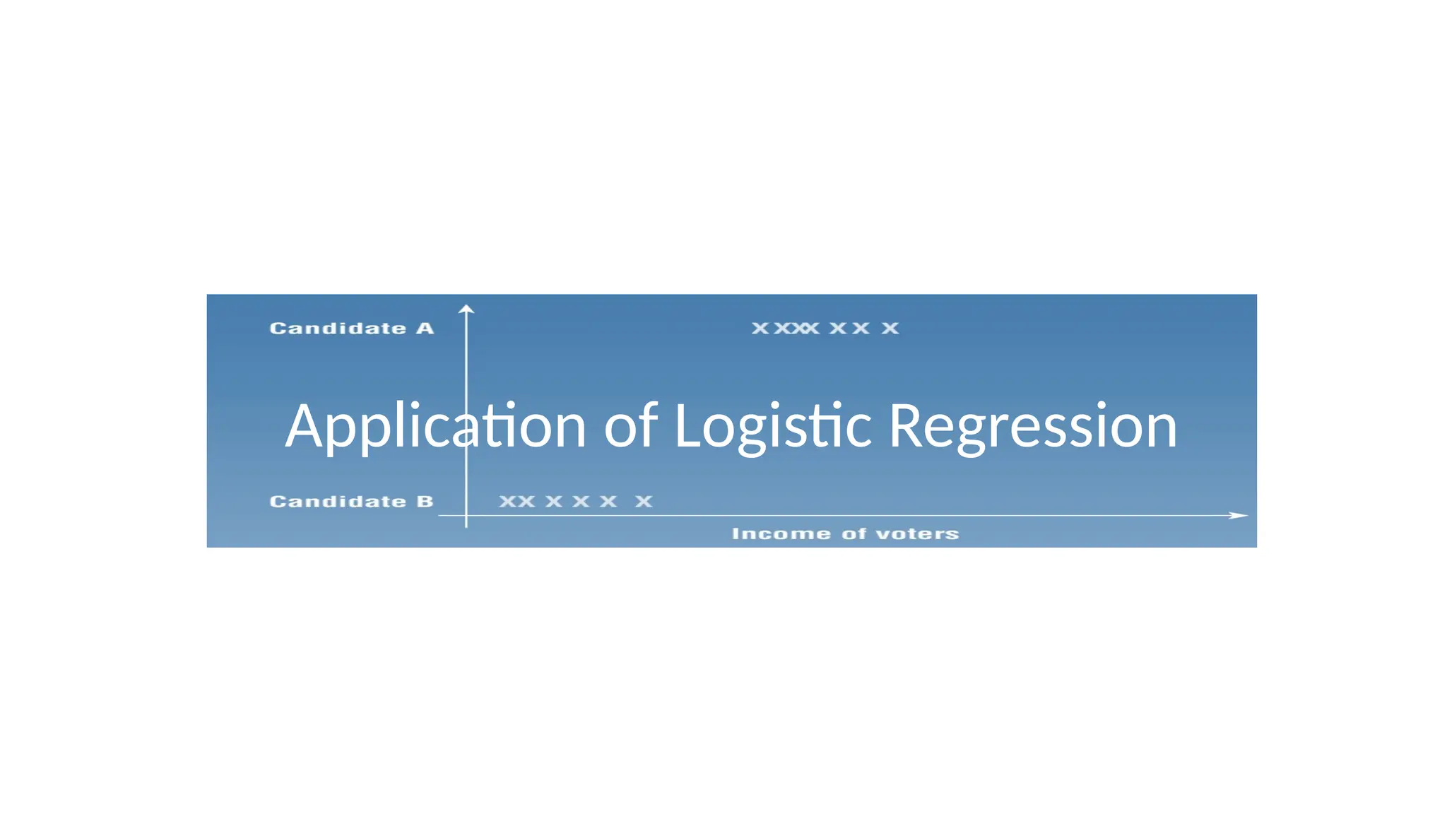
Logistic Regression • Consider the example shown in Fig. • Suppose that you have a dataset containing information about voter income and voting preferences. • For this dataset, you can see that low-income voters tend to vote for candidate B, while high-income voters tend to favor candidate A. • We would be very interested in trying to predict which candidate future voters will vote for based on their income level. Classification Example

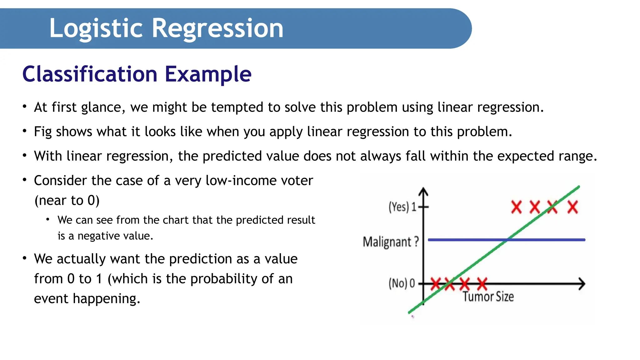
Logistic Regression • At first glance, we might be tempted to solve this problem using linear regression. • Fig shows what it looks like when you apply linear regression to this problem. • With linear regression, the predicted value does not always fall within the expected range. • Consider the case of a very low-income voter (near to 0) • We can see from the chart that the predicted result is a negative value. • We actually want the prediction as a value from 0 to 1 (which is the probability of an event happening. Classification Example

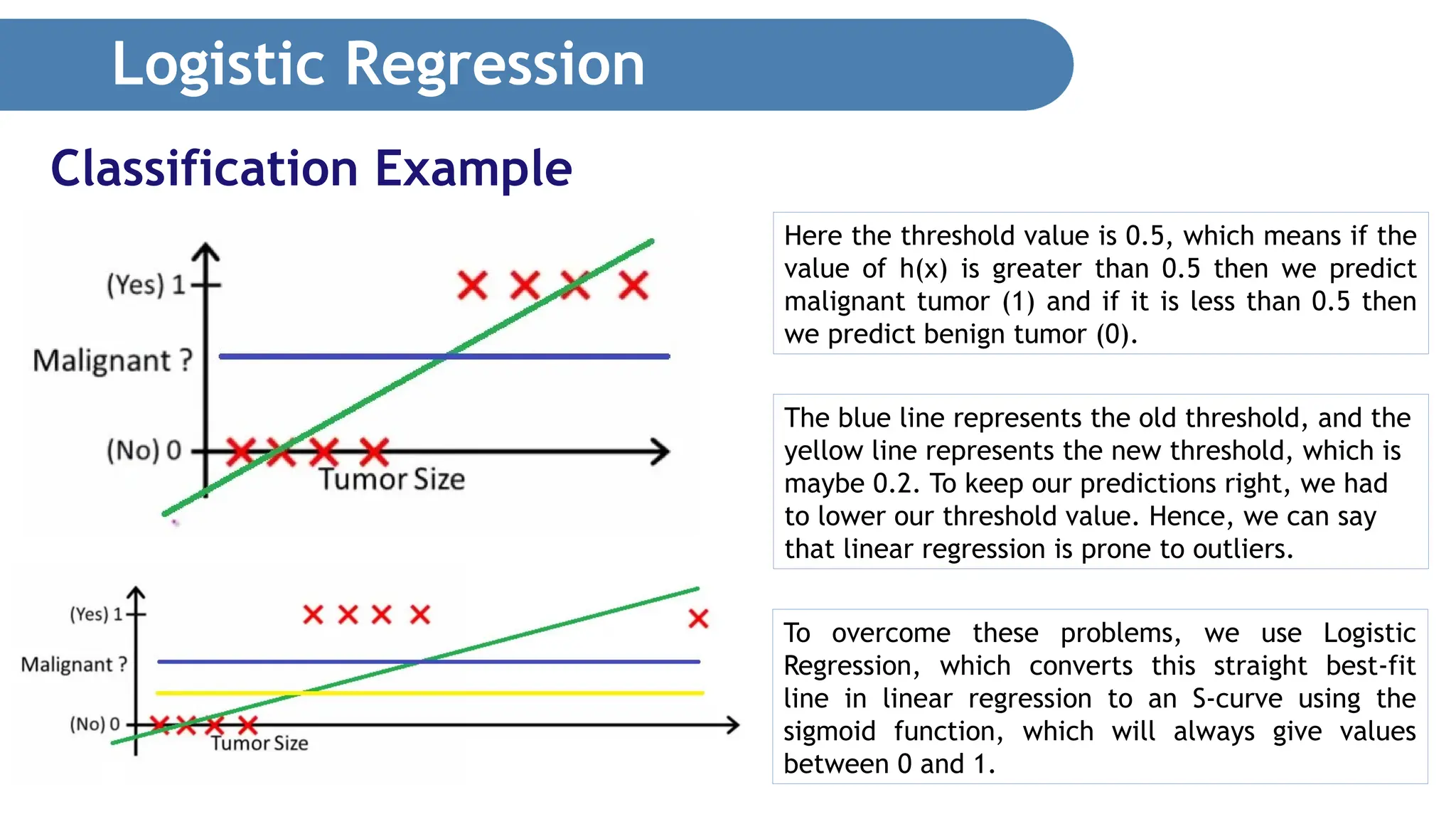
Logistic Regression Classification Example Here the threshold value is 0.5, which means if the value of h(x) is greater than 0.5 then we predict malignant tumor (1) and if it is less than 0.5 then we predict benign tumor (0). The blue line represents the old threshold, and the yellow line represents the new threshold, which is maybe 0.2. To keep our predictions right, we had to lower our threshold value. Hence, we can say that linear regression is prone to outliers. To overcome these problems, we use Logistic Regression, which converts this straight best-fit line in linear regression to an S-curve using the sigmoid function, which will always give values between 0 and 1.

Logistic Regression • Logistic Regression (also called Logit Regression) • Logistic Regression is commonly used to estimate the probability that an instance belongs to a particular class • E.g., what is the probability that this email is spam? • Estimate the probability • If greater than 50%, • then the model predicts that the instance belongs to that class (called the positive class, labeled “1”), • else • it predicts that it does not (i.e., it belongs to the negative class, labeled “0”). • This makes logistic regression a binary classifier. Overview

Logistic Regression • Independent observations: Each observation is independent of the other. meaning there is no correlation between any input variables. • Binary dependent variables: It takes the assumption that the dependent variable must be binary or dichotomous, meaning it can take only two values. For more than two categories SoftMax functions are used. • Linearity relationship between independent variables and log odds: The relationship between the independent variables and the log odds of the dependent variable should be linear. • No outliers: There should be no outliers in the dataset. • Large sample size: The sample size is sufficiently large Assumptions

Logistic Regression • Independent variables: The input characteristics or predictor factors applied to the dependent variable’s predictions. • Dependent variable: The target variable in a logistic regression model, which we are trying to predict. • Logistic function: The formula used to represent how the independent and dependent variables relate to one another. The logistic function transforms the input variables into a probability value between 0 and 1, which represents the likelihood of the dependent variable being 1 or 0. • Odds: It is the ratio of something occurring to something not occurring. it is different from probability as the probability is the ratio of something occurring to everything that could possibly occur. Terminologies involved in Logistic Regression

Logistic Regression • Log-odds: The log-odds, also known as the logit function, is the natural logarithm of the odds. In logistic regression, the log odds of the dependent variable are modeled as a linear combination of the independent variables and the intercept. • Coefficient: The logistic regression model’s estimated parameters, show how the independent and dependent variables relate to one another. • Intercept: A constant term in the logistic regression model, which represents the log odds when all independent variables are equal to zero. • Maximum likelihood estimation: The method used to estimate the coefficients of the logistic regression model, which maximizes the likelihood of observing the data given the model. Terminologies involved in Logistic Regression

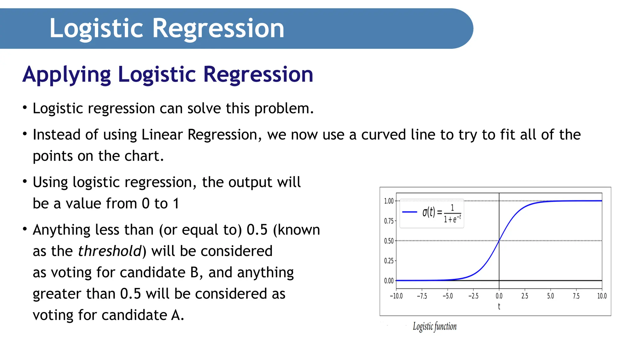
Logistic Regression • Logistic regression can solve this problem. • Instead of using Linear Regression, we now use a curved line to try to fit all of the points on the chart. • Using logistic regression, the output will be a value from 0 to 1 • Anything less than (or equal to) 0.5 (known as the threshold) will be considered as voting for candidate B, and anything greater than 0.5 will be considered as voting for candidate A. Applying Logistic Regression

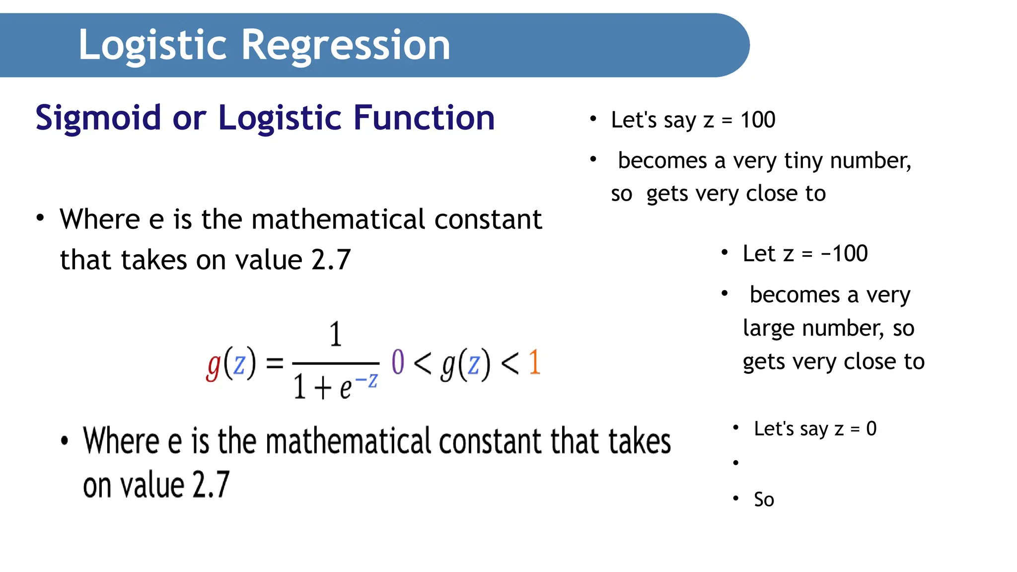
Logistic Regression • Where e is the mathematical constant that takes on value 2.7 Sigmoid or Logistic Function • Let's say z = 100 • becomes a very tiny number, so gets very close to • Let z = −100 • becomes a very large number, so gets very close to • Let's say z = 0 • • So

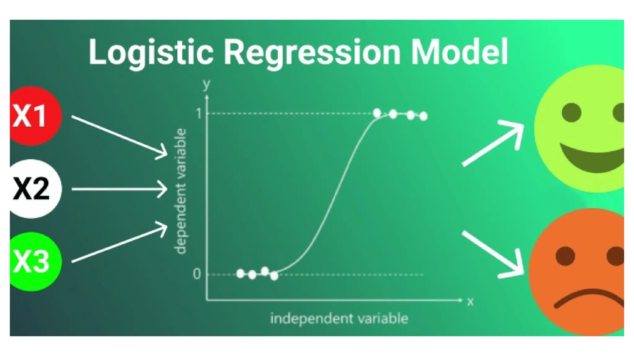
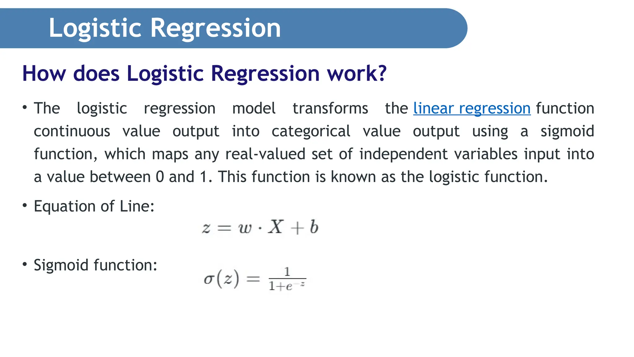
Logistic Regression • The logistic regression model transforms the linear regression function continuous value output into categorical value output using a sigmoid function, which maps any real-valued set of independent variables input into a value between 0 and 1. This function is known as the logistic function. • Equation of Line: • Sigmoid function: How does Logistic Regression work?

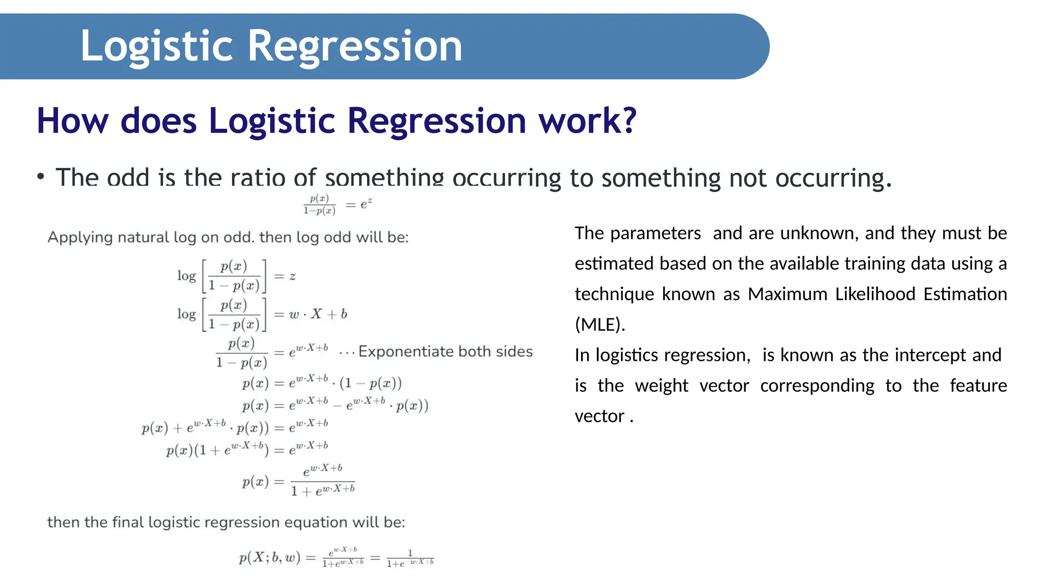
Logistic Regression • The odd is the ratio of something occurring to something not occurring. How does Logistic Regression work? The parameters and are unknown, and they must be estimated based on the available training data using a technique known as Maximum Likelihood Estimation (MLE). In logistics regression, is known as the intercept and is the weight vector corresponding to the feature vector .

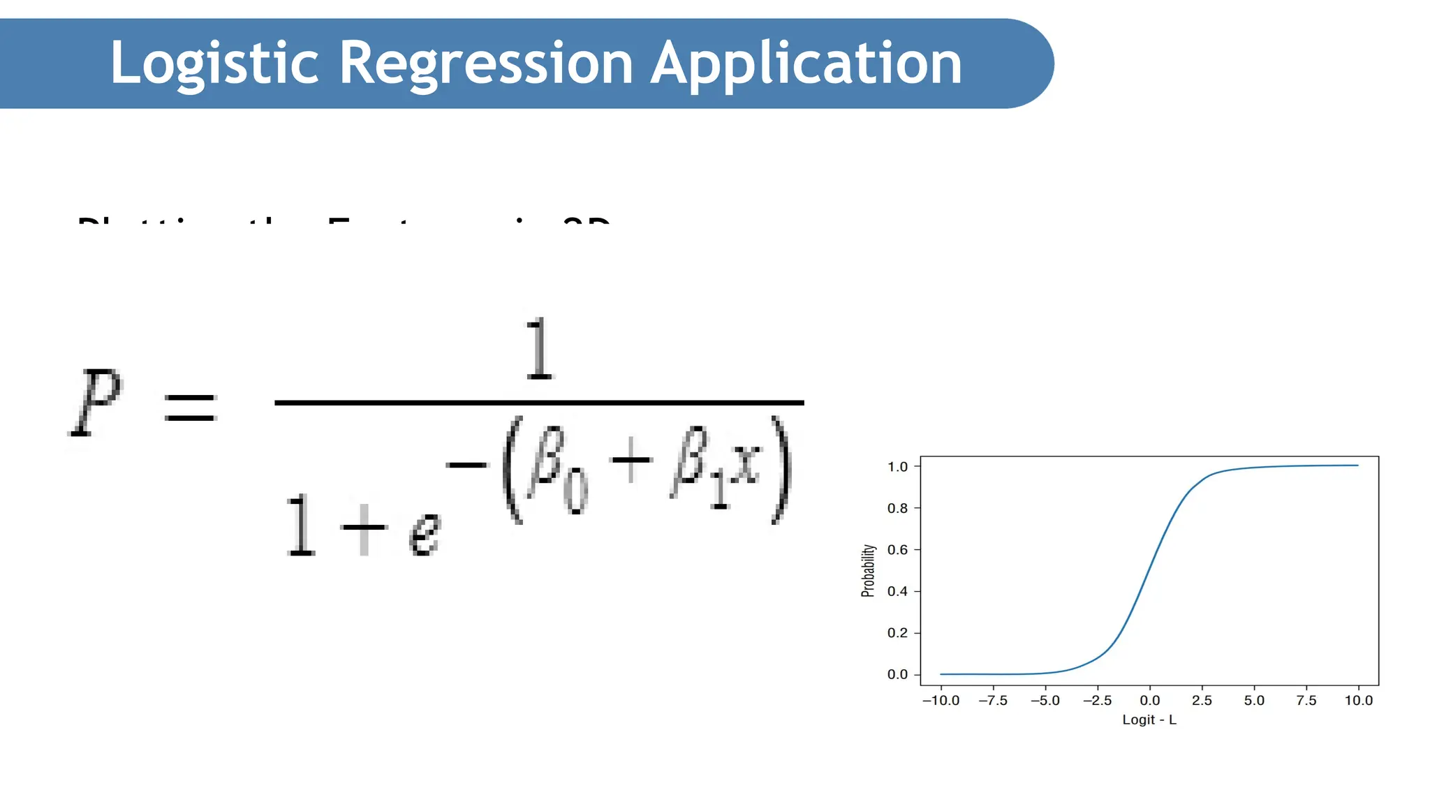
Logistic Regression • The following code snippet shows how the sigmoid curve is obtained: def sigmoid(x): return (1 / (1 + np.exp(-x))) x = np.arange(-10, 10, 0.0001) y = [sigmoid(n) for n in x] plt.plot(x,y) plt.xlabel("Logit - L") plt.ylabel("Probability") • Fig shows the sigmoid curve. Plotting Sigmoid Curve

Application of Logistic Regression

Logistic Regression Application • Scikit-learn includes the Breast Cancer Wisconsin (Diagnostic) Data Set. • It is a popular dataset often used for illustrating binary classifications. • The dataset contains 569 samples and 30 features • These features are computed from a digitized image of a fine needle aspirate (FNA) of a breast mass. • The label (outcome) of the dataset is a binary classification—M for malignant or B for benign. • For more information: • https://archive.ics.uci.edu/ml/datasets/Breast+Cancer+Wisconsin+(Diagnostic) Breast Cancer Dataset

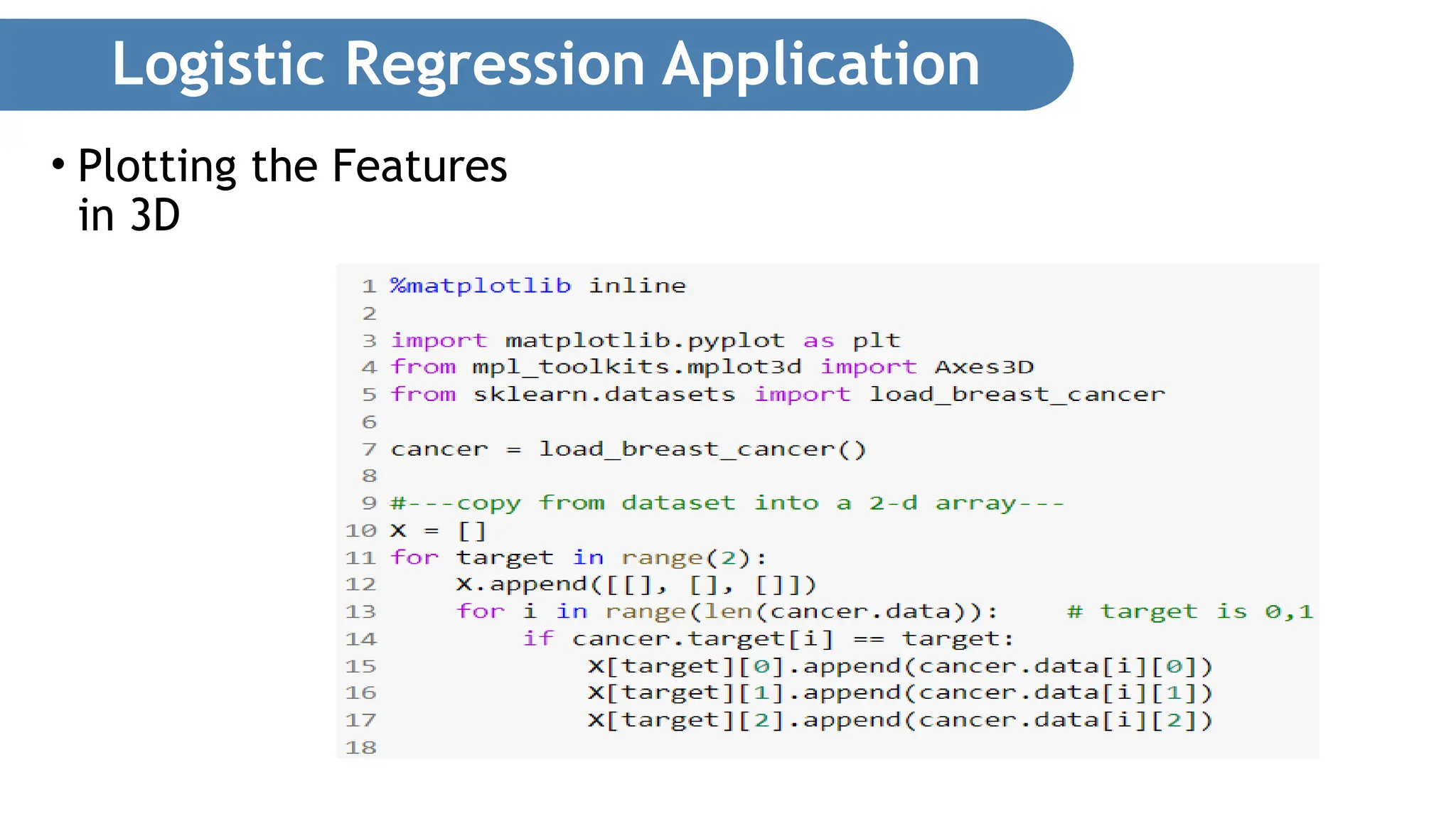
Logistic Regression Application • First, load the Breast Cancer dataset by first importing the datasets module from sklearn. • Then use the load _ breast _ cancer() function as follows: from sklearn.datasets import load_breast_cancer cancer = load_breast_cancer() Examining the Relationship Between Features

Logistic Regression Application • Let’s plot the first two features of the dataset in 2D and examine their relationships. • The following code snippet: • Loads the Breast Cancer dataset • Copies the first two features of the dataset into a two-dimensional list • Plots a scatter plot showing the distribution of points for the two features • Displays malignant growths in red and benign growths in blue Plotting the Features in 2D

Logistic Regression Application • Plotting the Features in 2D

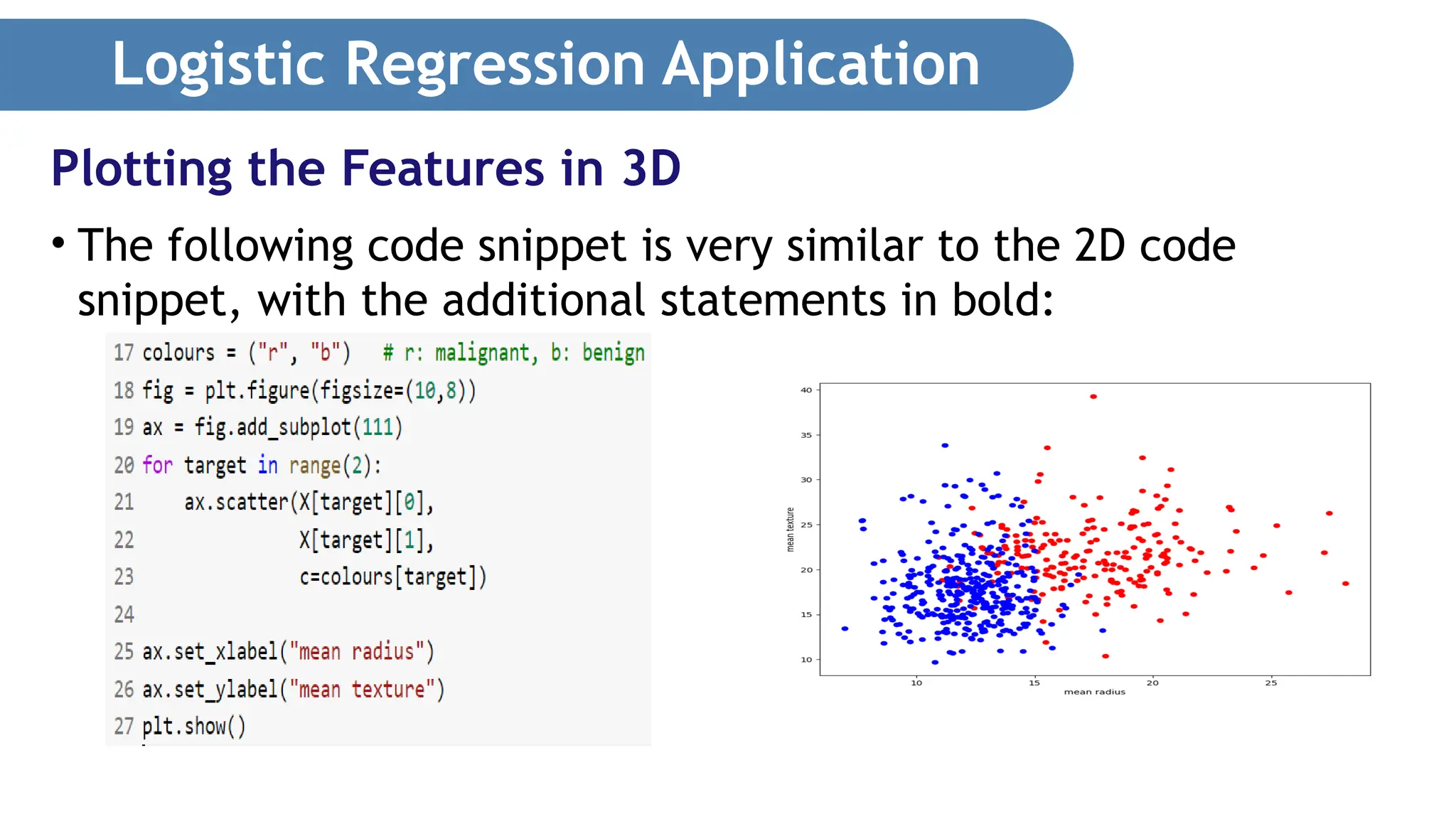
Logistic Regression Application • The following code snippet is very similar to the 2D code snippet, with the additional statements in bold: Plotting the Features in 3D

Logistic Regression Application • Plotting the Features in 3D

Logistic Regression Application • Running the following command displays the list of features of this dataset. • >>>cancer.feature_names • >>>array(['mean radius', 'mean texture', 'mean perimeter', 'mean area', 'mean smoothness', 'mean compactness', 'mean concavity', 'mean concave points', 'mean symmetry', 'mean fractal dimension', 'radius error', 'texture error', 'perimeter error', 'area error', 'smoothness error', 'compactness error', 'concavity error', 'concave points error', 'symmetry error', 'fractal dimension error', 'worst radius', 'worst texture', 'worst perimeter', 'worst area', 'worst smoothness', 'worst compactness', 'worst concavity', 'worst concave points', 'worst symmetry', 'worst fractal dimension'], dtype='<U23') Features of the Dataset

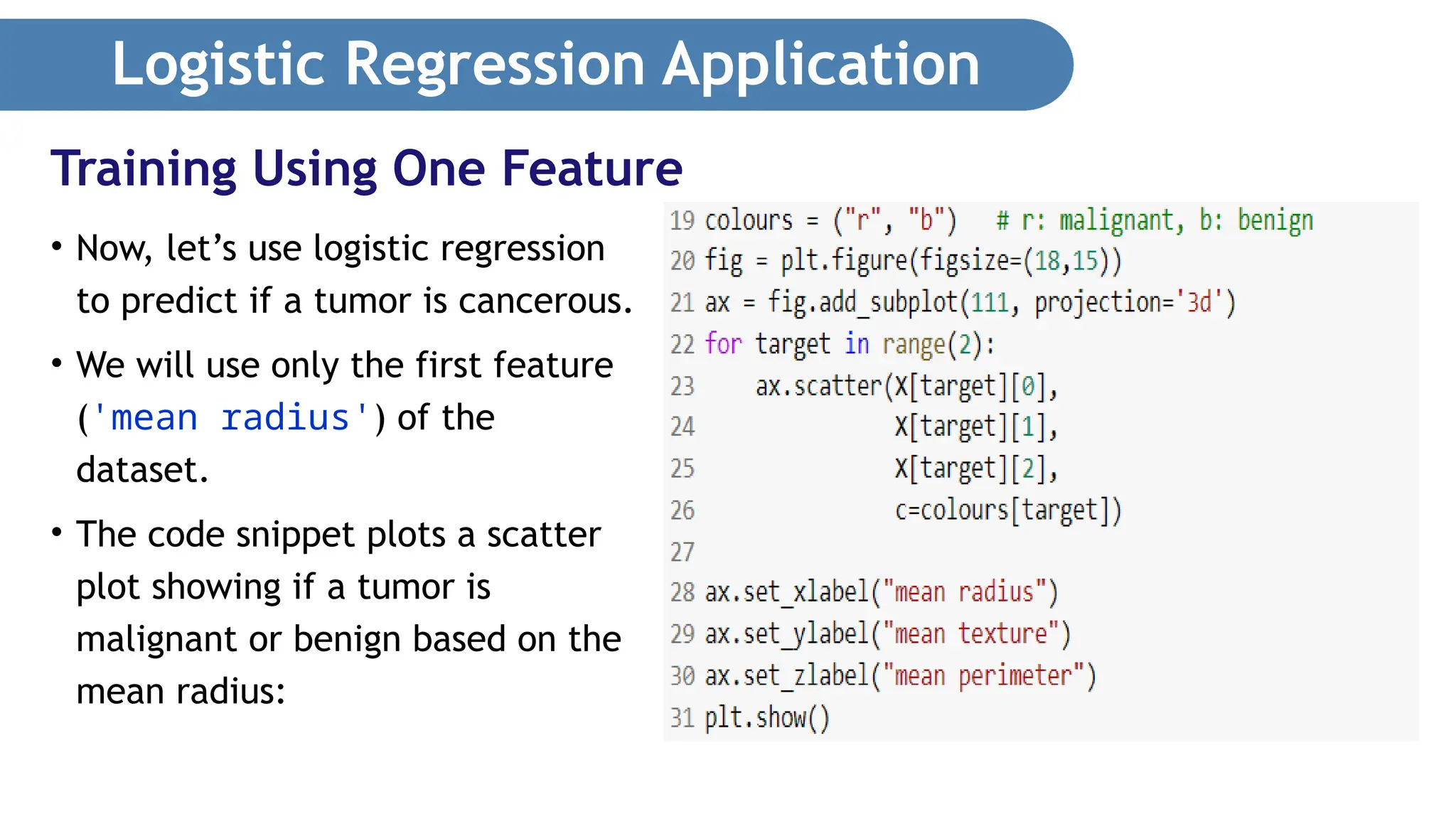
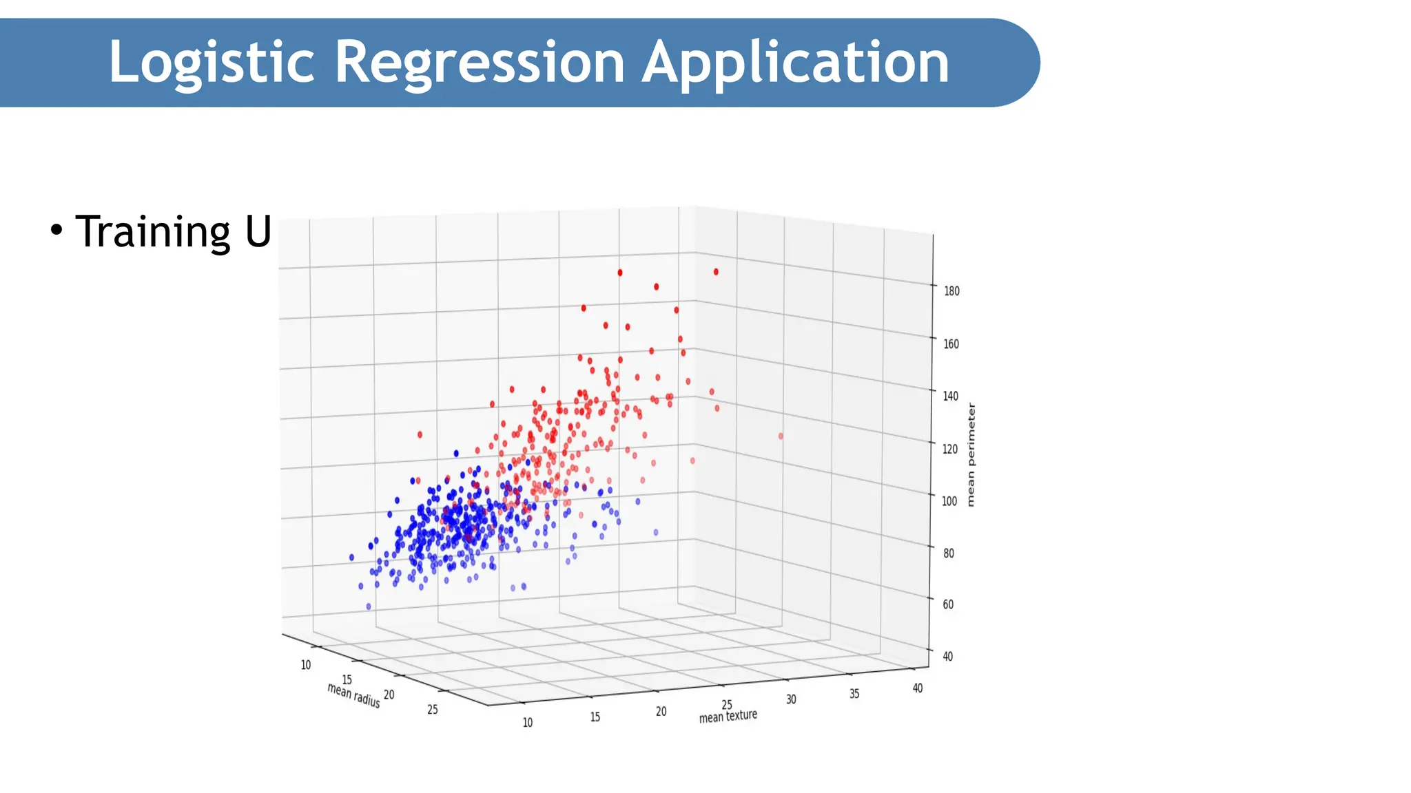
Logistic Regression Application • Now, let’s use logistic regression to predict if a tumor is cancerous. • We will use only the first feature ('mean radius') of the dataset. • The code snippet plots a scatter plot showing if a tumor is malignant or benign based on the mean radius: Training Using One Feature

Logistic Regression Application • Training Using One Feature

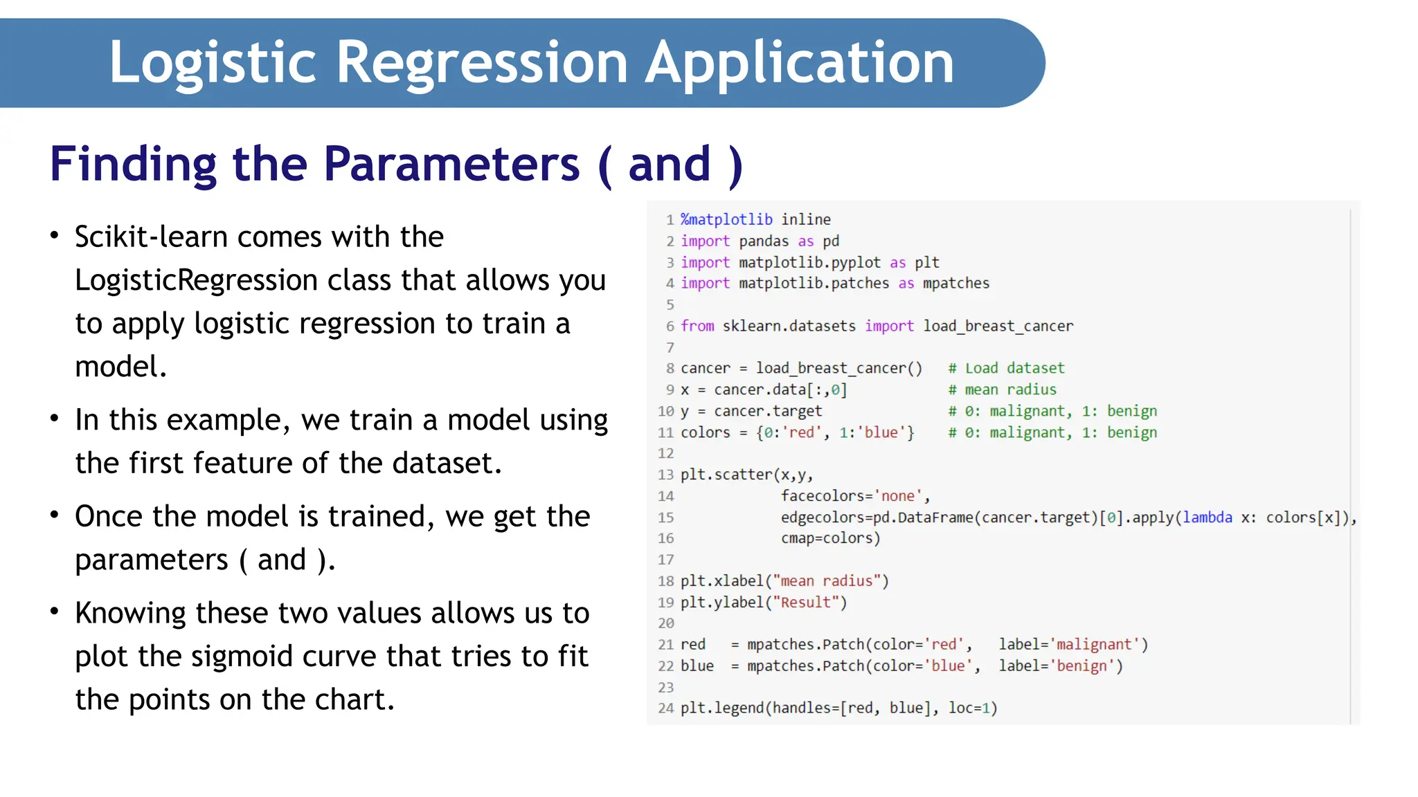
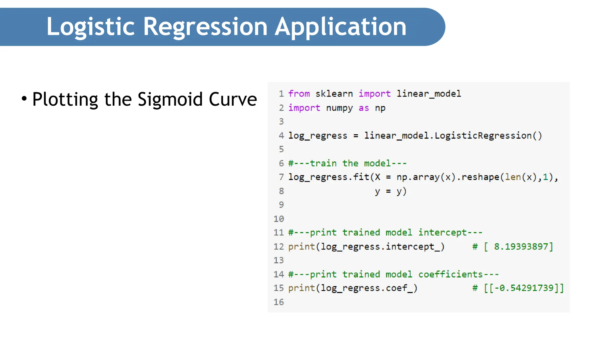
Logistic Regression Application • Scikit-learn comes with the LogisticRegression class that allows you to apply logistic regression to train a model. • In this example, we train a model using the first feature of the dataset. • Once the model is trained, we get the parameters ( and ). • Knowing these two values allows us to plot the sigmoid curve that tries to fit the points on the chart. Finding the Parameters ( and )

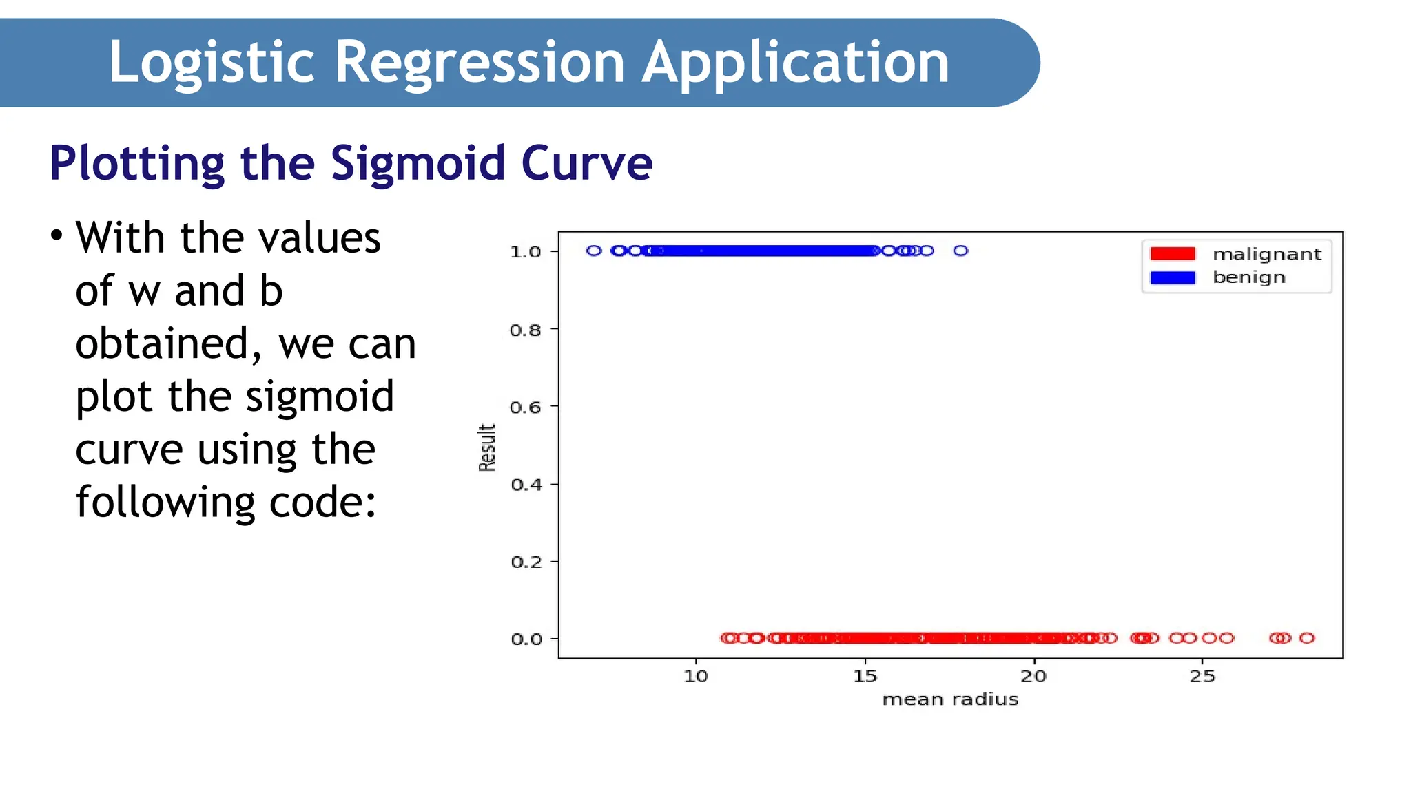
Logistic Regression Application • With the values of w and b obtained, we can plot the sigmoid curve using the following code: Plotting the Sigmoid Curve

Logistic Regression Application • Plotting the Sigmoid Curve

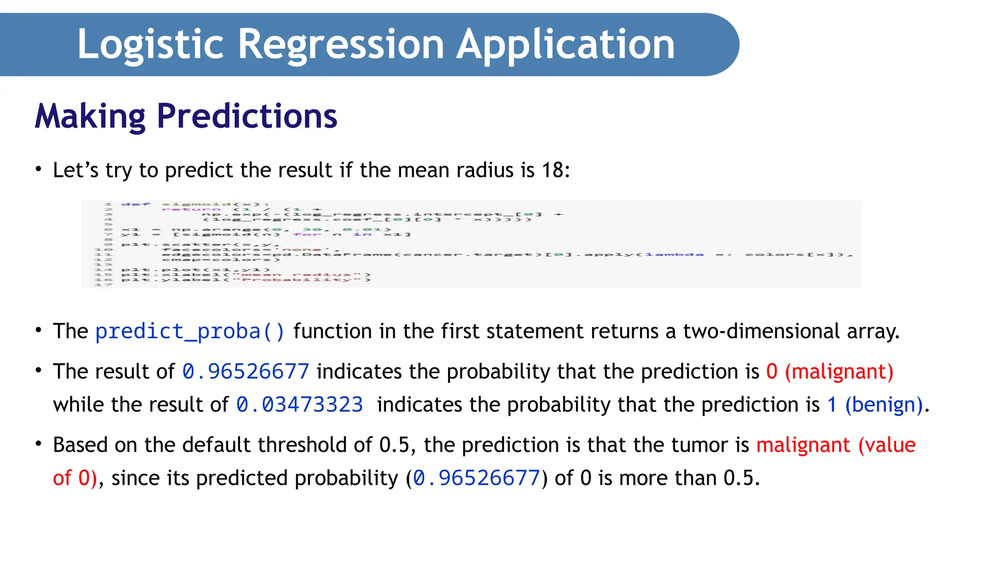
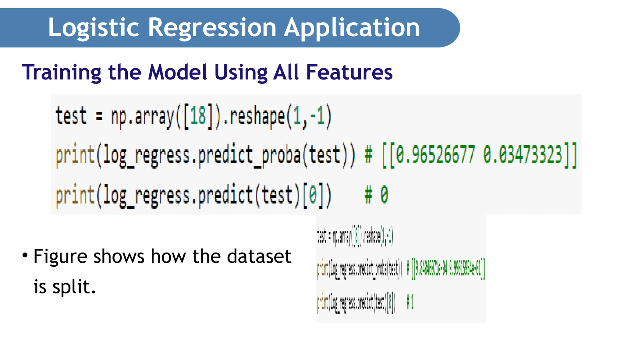
Logistic Regression Application • Let’s try to predict the result if the mean radius is 18: • The predict_proba() function in the first statement returns a two-dimensional array. • The result of 0.96526677 indicates the probability that the prediction is 0 (malignant) while the result of 0.03473323 indicates the probability that the prediction is 1 (benign). • Based on the default threshold of 0.5, the prediction is that the tumor is malignant (value of 0), since its predicted probability (0.96526677) of 0 is more than 0.5. Making Predictions

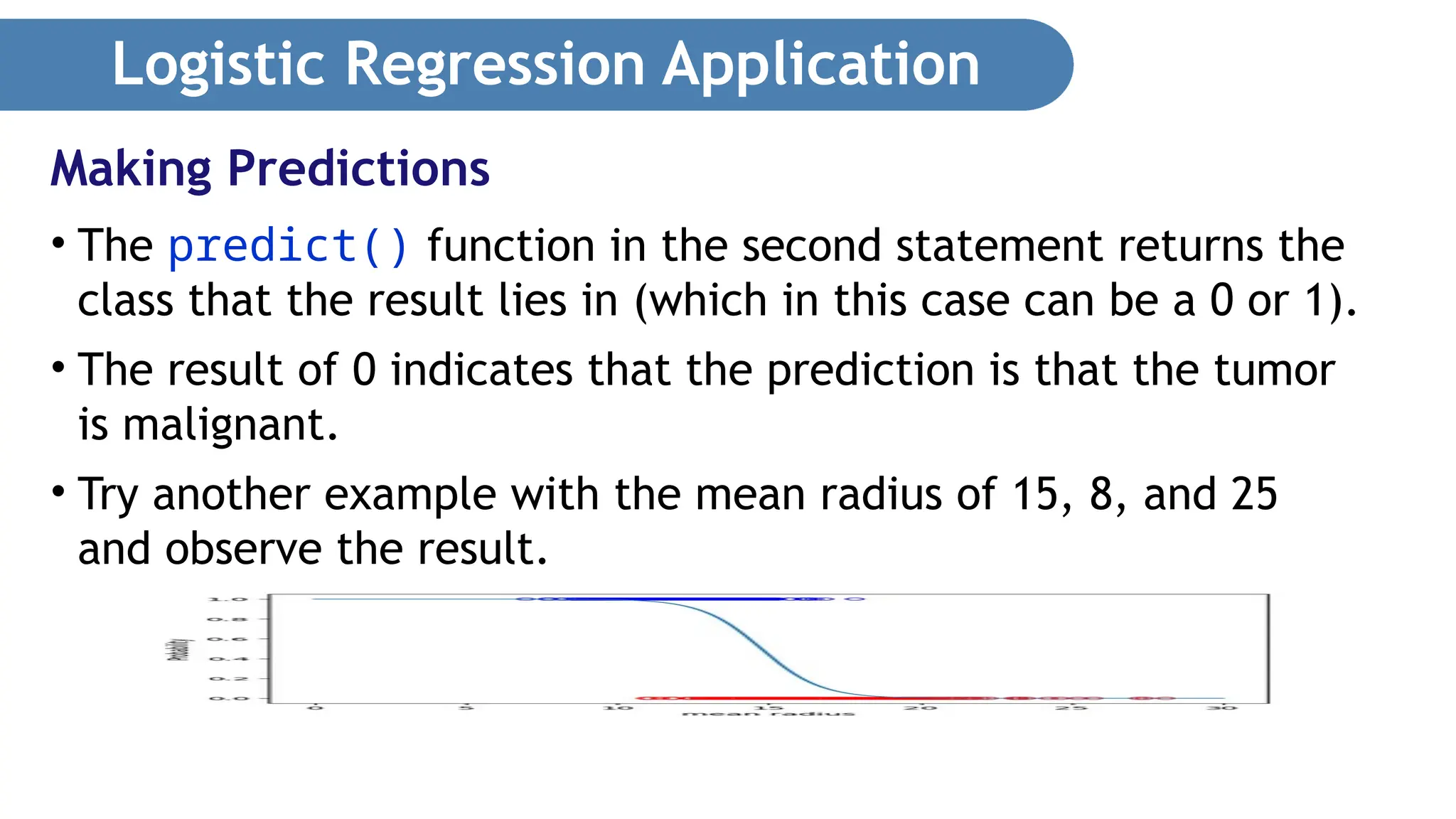
Logistic Regression Application • The predict() function in the second statement returns the class that the result lies in (which in this case can be a 0 or 1). • The result of 0 indicates that the prediction is that the tumor is malignant. • Try another example with the mean radius of 15, 8, and 25 and observe the result. Making Predictions

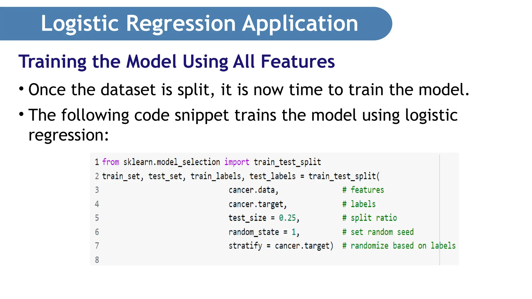
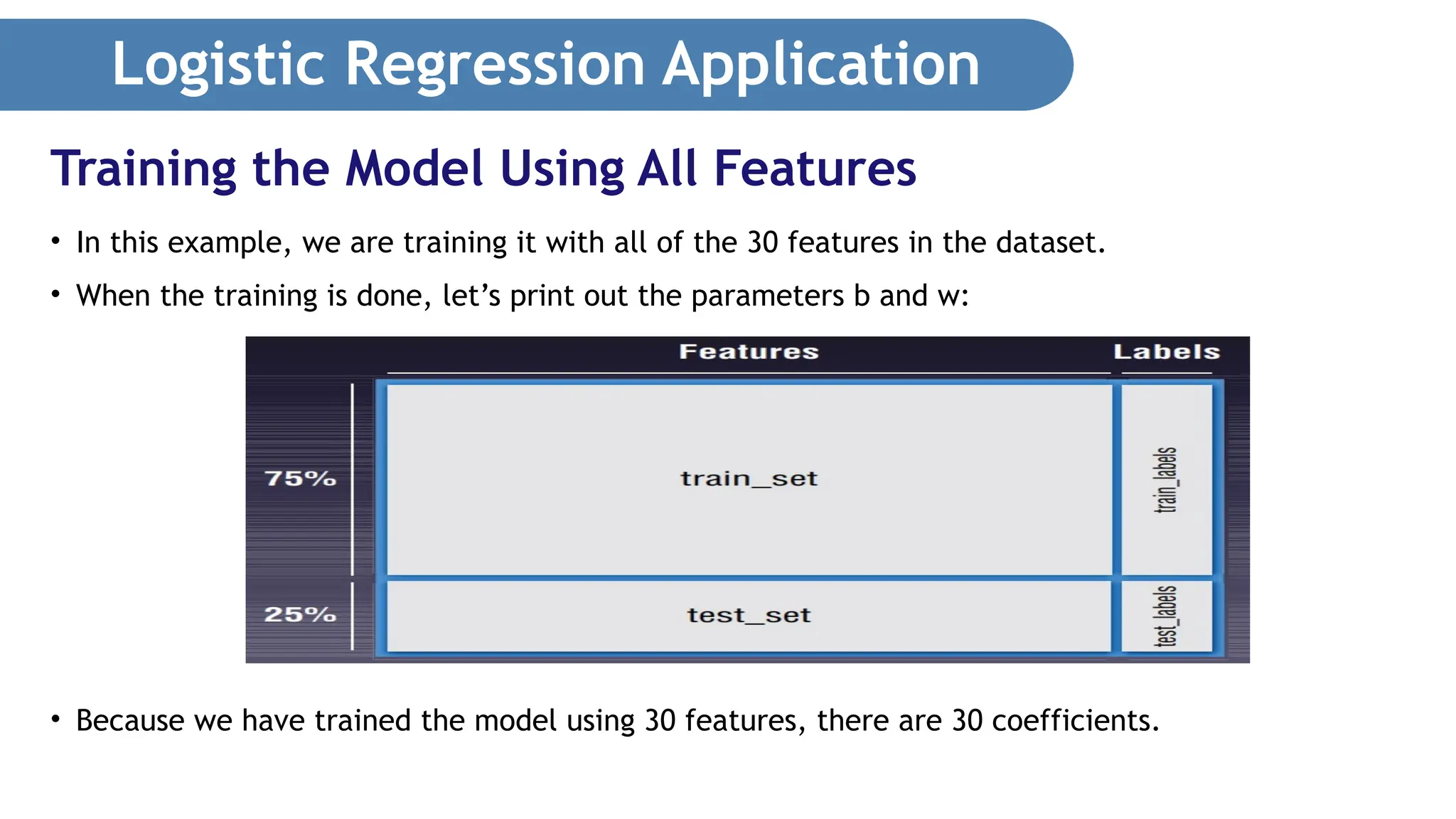
Logistic Regression Application • Let’s now try to train the model using all of the features and then see how well it can accurately perform the prediction. • First, load the dataset: from sklearn.datasets import load_breast_cancer cancer = load_breast_cancer() # Load dataset • Instead of training the model using all of the rows in the dataset, we are going to split it into two sets, one for training and one for testing, using train_test_split() function. • This function splits the data into training and test subsets randomly. • The following code snippet splits the dataset into a 75 percent training and 25 percent testing set: Training the Model Using All Features

Logistic Regression Application • Figure shows how the dataset is split. Training the Model Using All Features

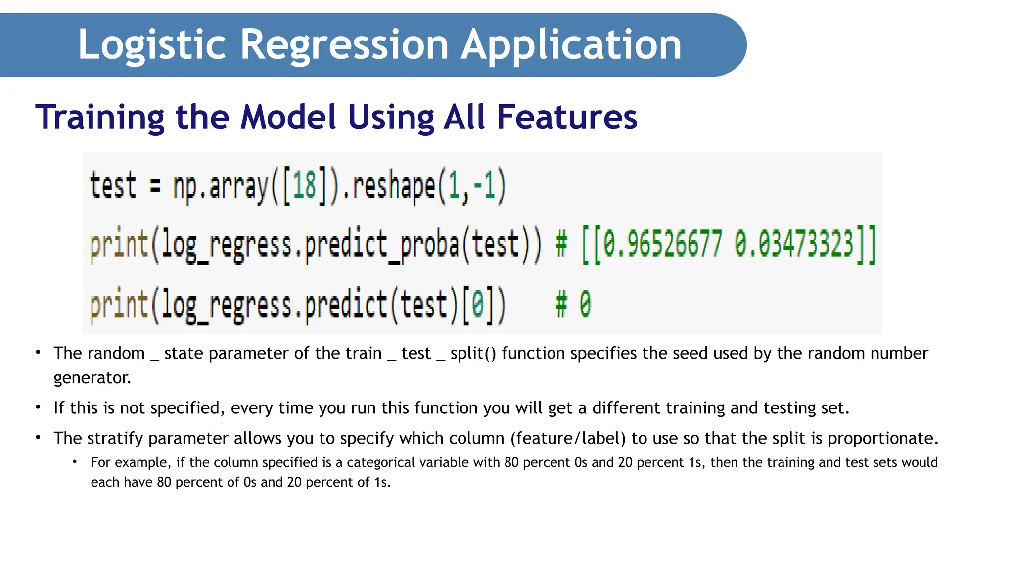
Logistic Regression Application • The random _ state parameter of the train _ test _ split() function specifies the seed used by the random number generator. • If this is not specified, every time you run this function you will get a different training and testing set. • The stratify parameter allows you to specify which column (feature/label) to use so that the split is proportionate. • For example, if the column specified is a categorical variable with 80 percent 0s and 20 percent 1s, then the training and test sets would each have 80 percent of 0s and 20 percent of 1s. Training the Model Using All Features

Logistic Regression Application • Once the dataset is split, it is now time to train the model. • The following code snippet trains the model using logistic regression: Training the Model Using All Features

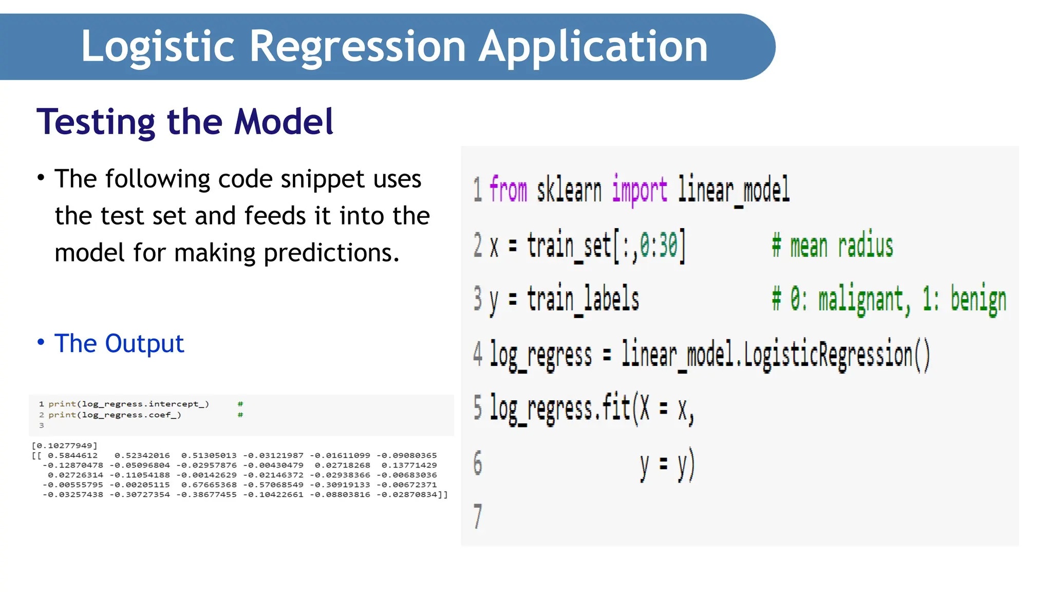
Logistic Regression Application • In this example, we are training it with all of the 30 features in the dataset. • When the training is done, let’s print out the parameters b and w: • Because we have trained the model using 30 features, there are 30 coefficients. Training the Model Using All Features

Logistic Regression Application • The following code snippet uses the test set and feeds it into the model for making predictions. • The Output Testing the Model

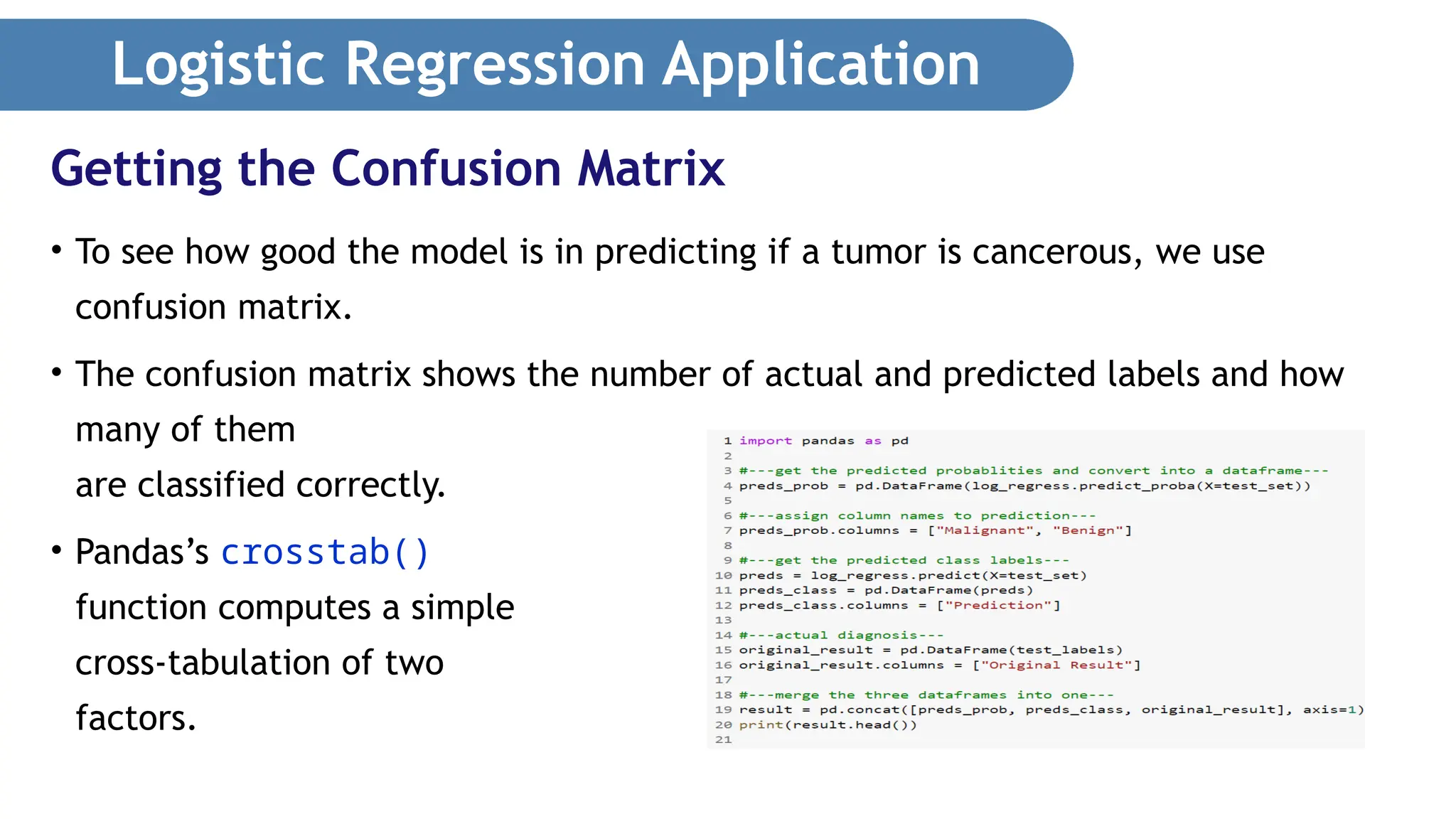
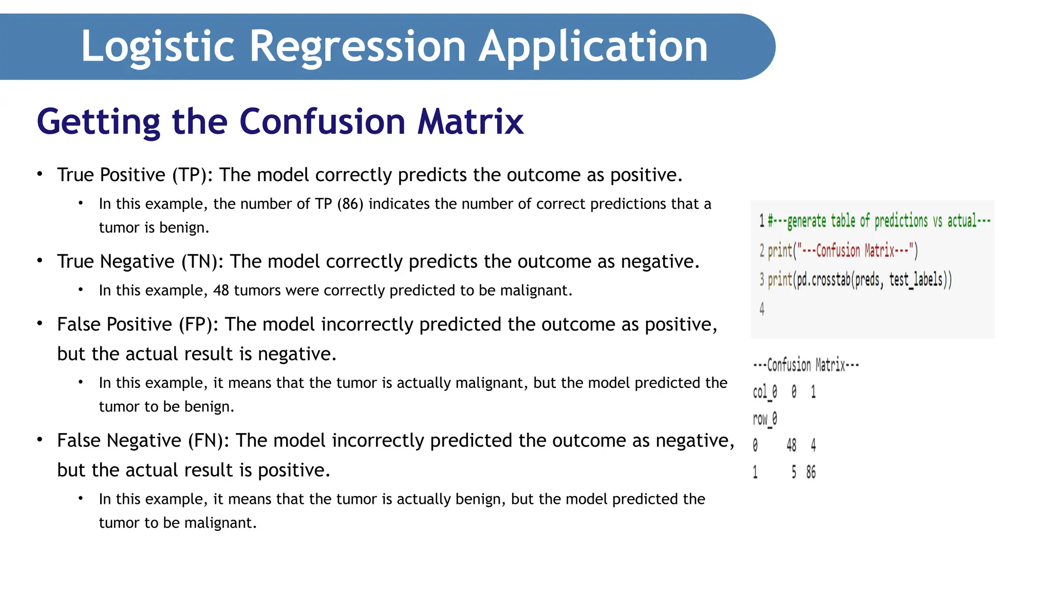
Logistic Regression Application • To see how good the model is in predicting if a tumor is cancerous, we use confusion matrix. • The confusion matrix shows the number of actual and predicted labels and how many of them are classified correctly. • Pandas’s crosstab() function computes a simple cross-tabulation of two factors. Getting the Confusion Matrix

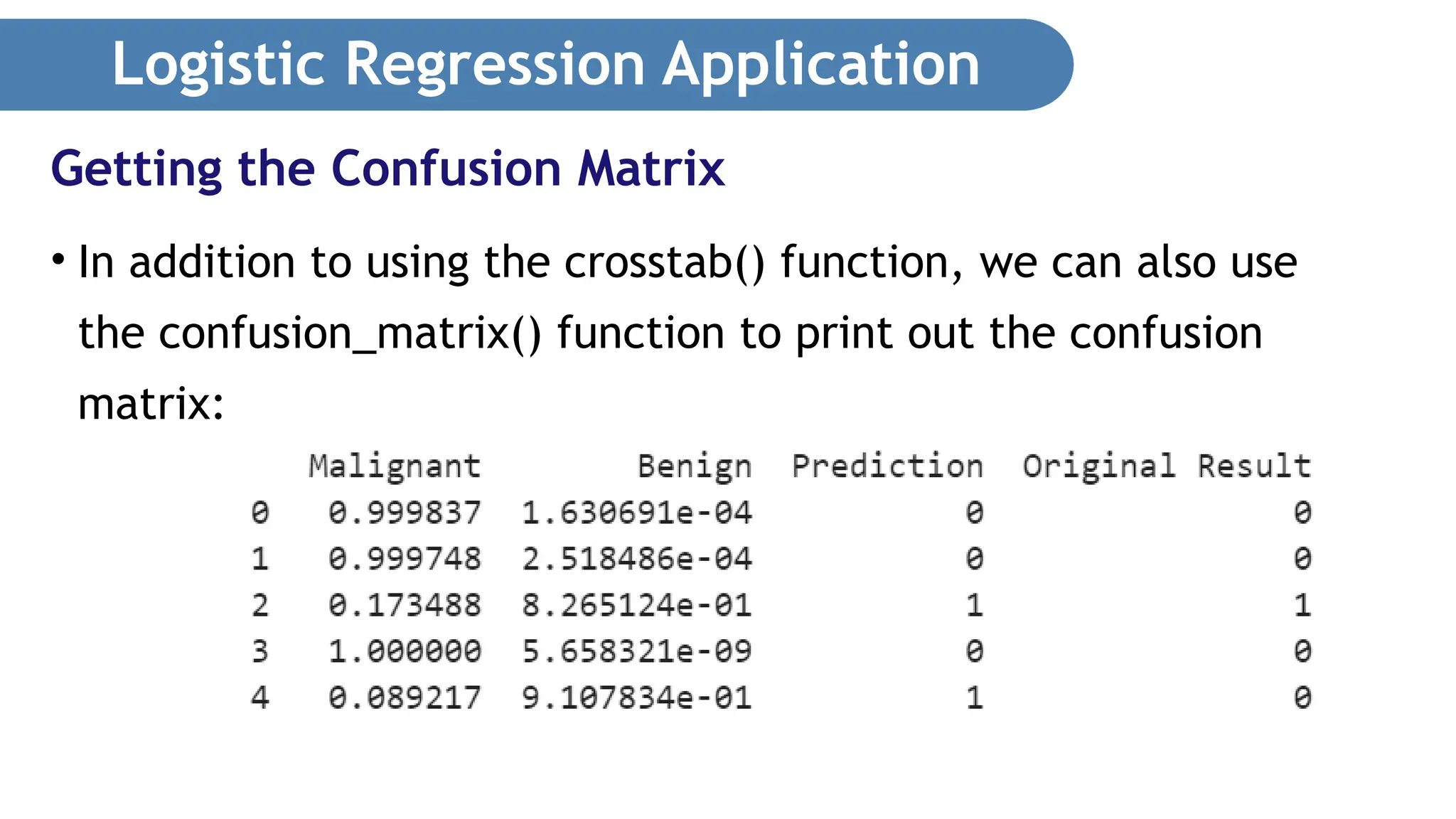
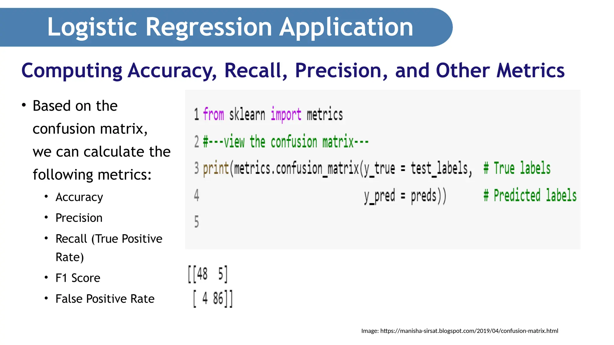
Logistic Regression Application • In addition to using the crosstab() function, we can also use the confusion_matrix() function to print out the confusion matrix: Getting the Confusion Matrix

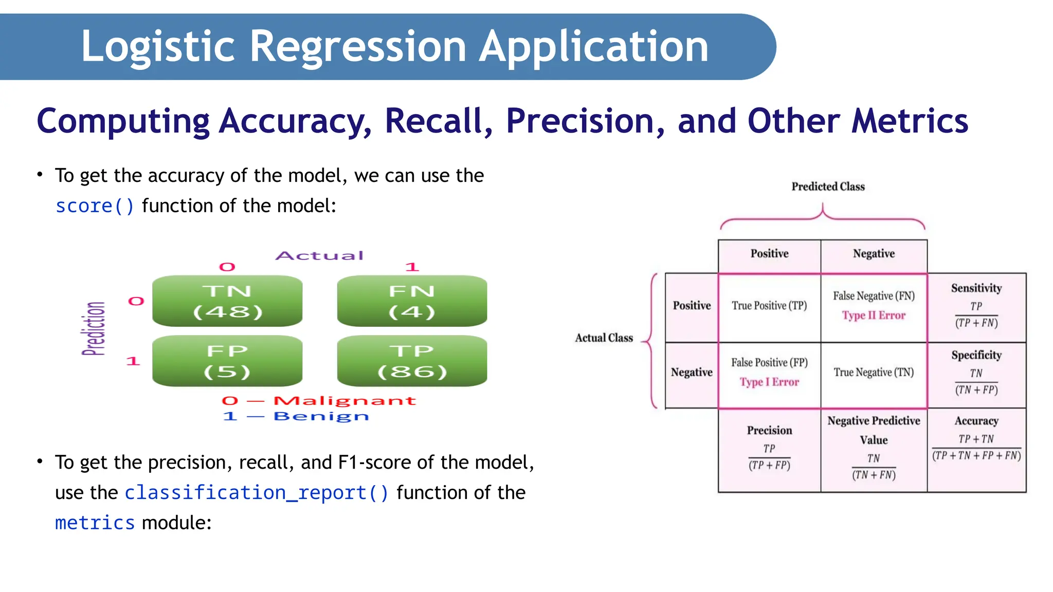
Logistic Regression Application • The output is interpreted as shown below: • The columns represent the actual diagnosis (0 for malignant and 1 for benign). • The rows represent the prediction. • Each individual box represents one of the following: • True Negative (TN), True Positive (TP), False Negative (FN), False Positive (FP) Getting the Confusion Matrix

Logistic Regression Application • True Positive (TP): The model correctly predicts the outcome as positive. • In this example, the number of TP (86) indicates the number of correct predictions that a tumor is benign. • True Negative (TN): The model correctly predicts the outcome as negative. • In this example, 48 tumors were correctly predicted to be malignant. • False Positive (FP): The model incorrectly predicted the outcome as positive, but the actual result is negative. • In this example, it means that the tumor is actually malignant, but the model predicted the tumor to be benign. • False Negative (FN): The model incorrectly predicted the outcome as negative, but the actual result is positive. • In this example, it means that the tumor is actually benign, but the model predicted the tumor to be malignant. Getting the Confusion Matrix

Logistic Regression Application • Based on the confusion matrix, we can calculate the following metrics: • Accuracy • Precision • Recall (True Positive Rate) • F1 Score • False Positive Rate Computing Accuracy, Recall, Precision, and Other Metrics Image: https://manisha-sirsat.blogspot.com/2019/04/confusion-matrix.html

Logistic Regression Application • To understand the concept of precision and recall, consider the following scenario • If a malignant tumor is represented as negative and a benign tumor is represented as positive, then: • If the precision or recall is high, it means that more patients with benign tumors are diagnosed correctly, which indicates that the algorithm is good. • If the precision is low, it means that more patients with malignant tumors are diagnosed as benign. • If the recall is low, it means that more patients with benign tumors are diagnosed as malignant. Computing Accuracy, Recall, Precision, and Other Metrics

Logistic Regression Application • Having a low precision is more serious than a low recall (although wrongfully diagnosed as having breast cancer when you do not have it will likely result in unnecessary treatment and mental anguish) because it causes the patient to miss treatment and potentially causes death. • Hence, for cases like diagnosing breast cancer, it’s important to consider both the precision and recall metrics when evaluating the effectiveness of an ML algorithm. Computing Accuracy, Recall, Precision, and Other Metrics

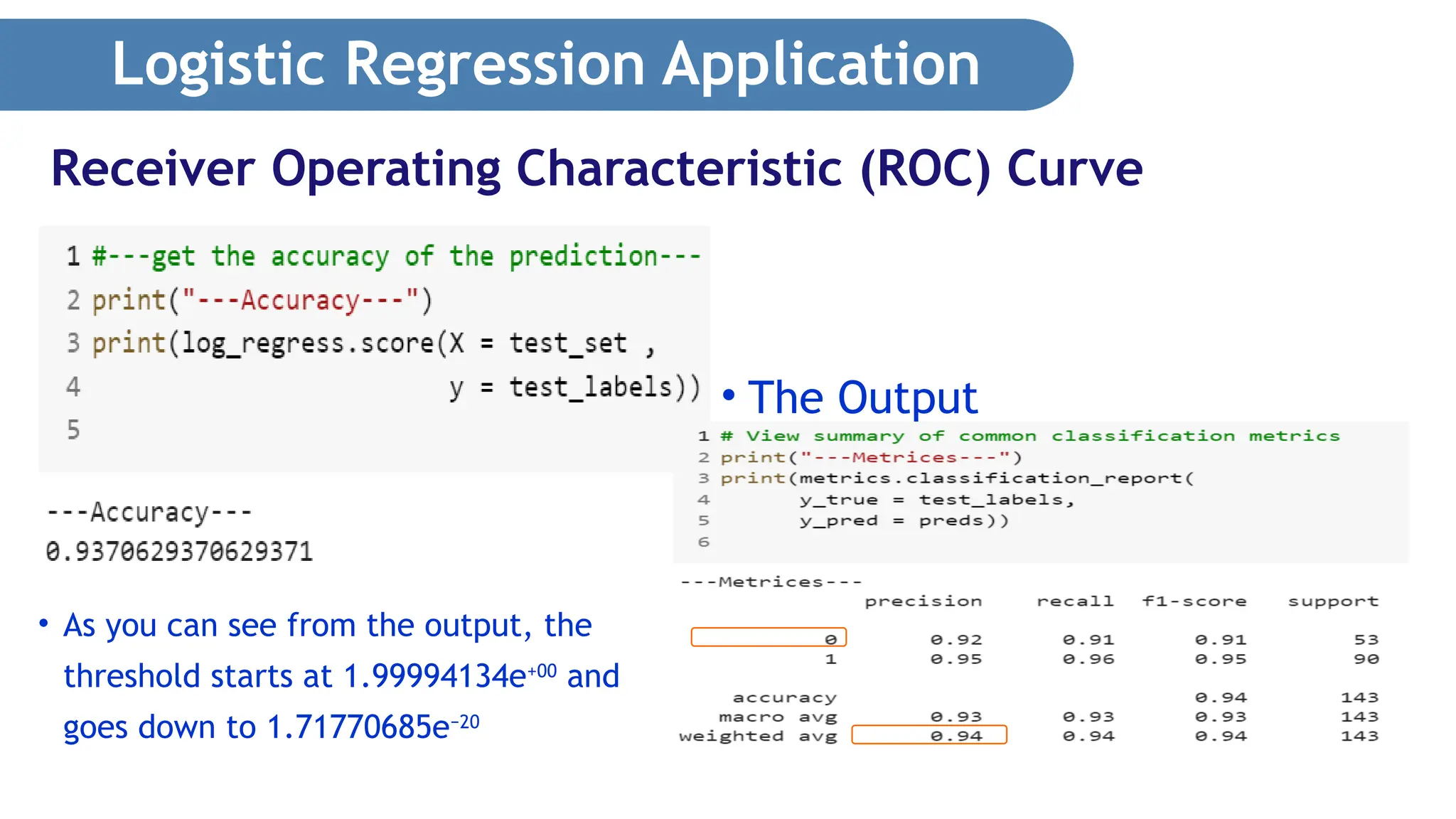
Logistic Regression Application • To get the accuracy of the model, we can use the score() function of the model: • To get the precision, recall, and F1-score of the model, use the classification_report() function of the metrics module: Computing Accuracy, Recall, Precision, and Other Metrics

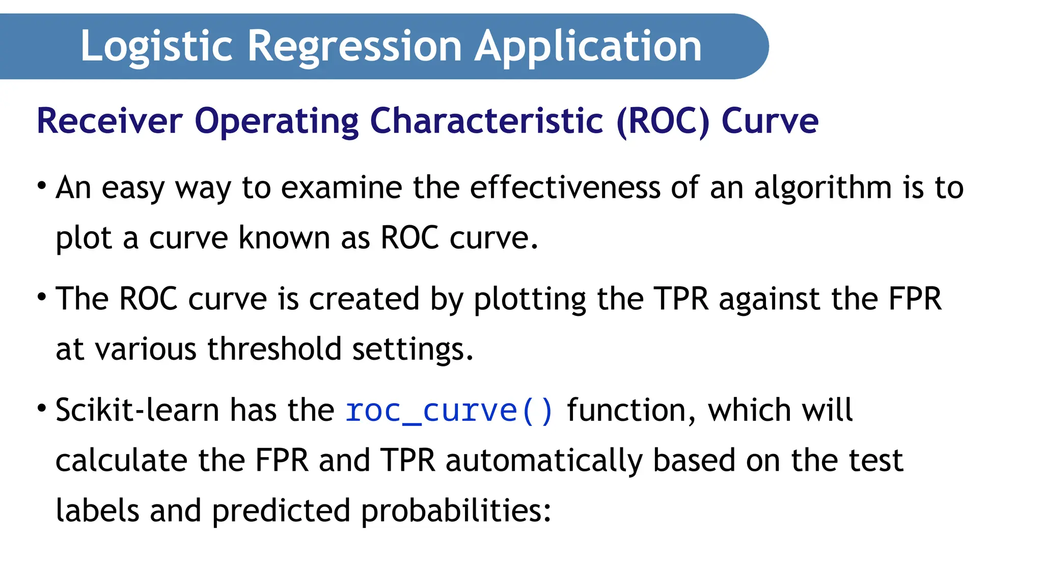
Logistic Regression Application • An easy way to examine the effectiveness of an algorithm is to plot a curve known as ROC curve. • The ROC curve is created by plotting the TPR against the FPR at various threshold settings. • Scikit-learn has the roc_curve() function, which will calculate the FPR and TPR automatically based on the test labels and predicted probabilities: Receiver Operating Characteristic (ROC) Curve

Logistic Regression Application • The Output Receiver Operating Characteristic (ROC) Curve • As you can see from the output, the threshold starts at 1.99994134e+00 and goes down to 1.71770685e−20

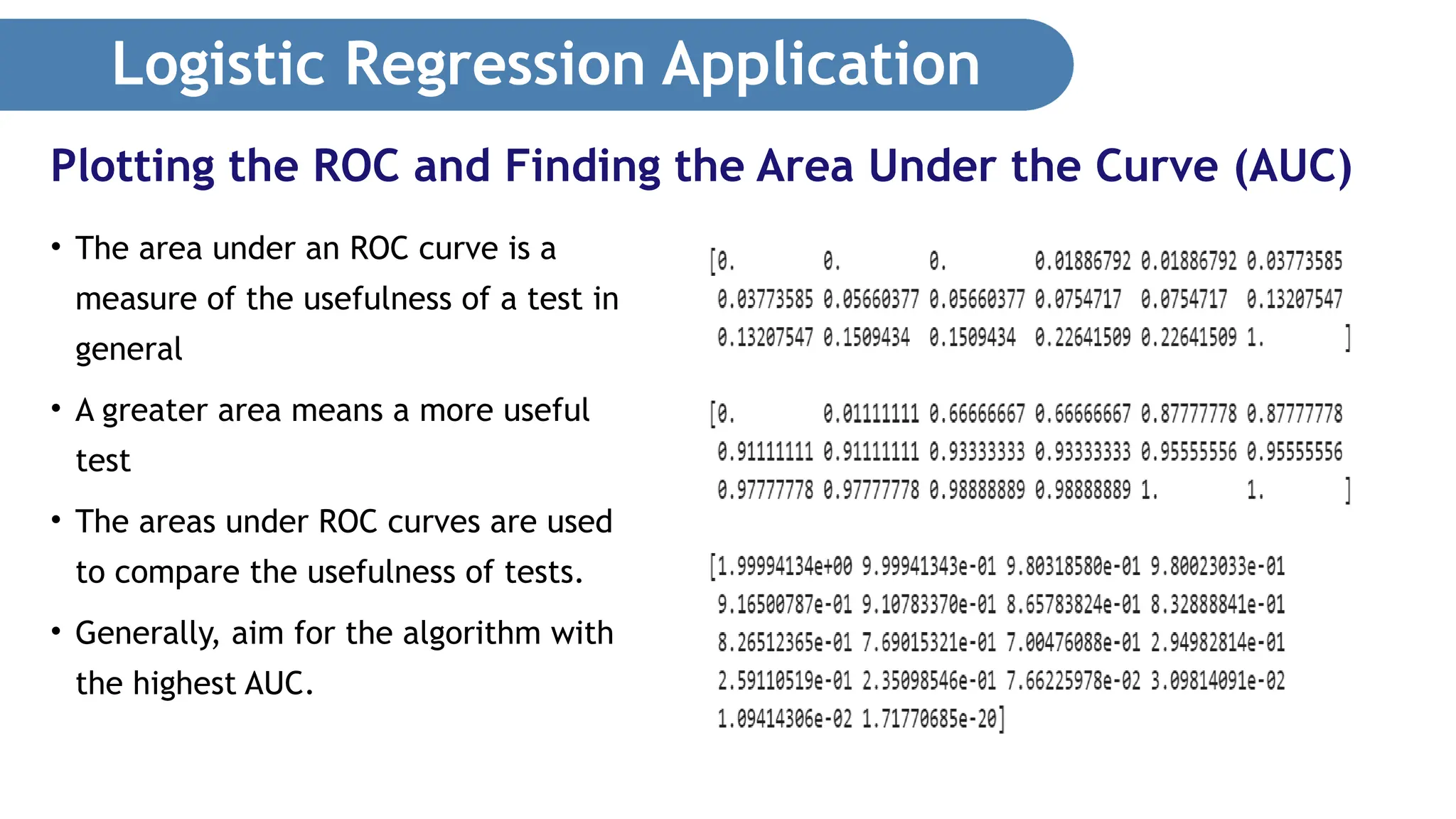
Logistic Regression Application • To plot the ROC, we use matplotlib to plot a line chart using the values stored in the fpr and tpr variables. • We can use the auc() function to find the area under the ROC: Plotting the ROC and Finding the Area Under the Curve (AUC)

Logistic Regression Application • The area under an ROC curve is a measure of the usefulness of a test in general • A greater area means a more useful test • The areas under ROC curves are used to compare the usefulness of tests. • Generally, aim for the algorithm with the highest AUC. Plotting the ROC and Finding the Area Under the Curve (AUC)

Linear Regression vs Logistic Regression

Logistic Regression • Python Machine Learning by Wei-Meng Lee • https://www.geeksforgeeks.org/understanding-logistic-regress ion • https://www.analyticsvidhya.com/blog/2021/08/conceptual- understanding-of-logistic-regression-for-data-science-beginner s/ • https://www.javatpoint.com/logistic-regression-in-machine-le arning Reference

Logistic Regression in machine learning ppt

More Related Content

Similar to Logistic Regression in machine learning ppt

Recently uploaded

Logistic Regression in machine learning ppt