Downloaded 87 times


![Broadcasting >>>importnumpyasnp >>>a=np.array([0,1,2,3]) >>>a*3 array([0,3,6,9]) >>>np.exp(a) array([ 1. , 2.71828183, 7.3890561, 20.08553692]) expis called a universal function. 10 / 26](https://image.slidesharecdn.com/introductiontonumpyformachinelearningprogrammers-150403214922-conversion-gate01/75/Introduction-to-NumPy-for-Machine-Learning-Programmers-10-2048.jpg)
![Broadcasting (2D) >>>importnumpyasnp >>>a=np.arange(9).reshape((3,3)) >>>b=np.array([1,2,3]) >>>a array([[0,1,2], [3,4,5], [6,7,8]]) >>>b array([1,2,3]) >>>a*b array([[0, 2, 6], [3, 8,15], [6,14,24]]) 11 / 26](https://image.slidesharecdn.com/introductiontonumpyformachinelearningprogrammers-150403214922-conversion-gate01/75/Introduction-to-NumPy-for-Machine-Learning-Programmers-11-2048.jpg)
![Indexing >>>importnumpyasnp >>>a=np.arange(10) >>>a array([0,1,2,3,4,5,6,7,8,9]) >>>indices=np.arange(0,10,2) >>>indices array([0,2,4,6,8]) >>>a[indices]=0 >>>a array([0,1,0,3,0,5,0,7,0,9]) >>>b=np.arange(100,600,100) >>>b array([100,200,300,400,500]) >>>a[indices]=b >>>a array([100, 1,200, 3,300, 5,400, 7,500, 9]) 12 / 26](https://image.slidesharecdn.com/introductiontonumpyformachinelearningprogrammers-150403214922-conversion-gate01/75/Introduction-to-NumPy-for-Machine-Learning-Programmers-12-2048.jpg)
![Boolean Indexing >>>a=np.array([1,2,3]) >>>b=np.array([False,True,True]) >>>a[b] array([2,3]) >>>c=np.arange(-3,4) >>>c array([-3,-2,-1, 0, 1, 2, 3]) >>>d=c>0 >>>d array([False,False,False,False, True, True, True],dtype=bool) >>>c[d] array([1,2,3]) >>>c[c>0] array([1,2,3]) >>>c[np.logical_and(c>=0,c%2==0)] array([0,2]) >>>c[np.logical_or(c>=0,c%2==0)] array([-2, 0, 1, 2, 3]) 13 / 26](https://image.slidesharecdn.com/introductiontonumpyformachinelearningprogrammers-150403214922-conversion-gate01/75/Introduction-to-NumPy-for-Machine-Learning-Programmers-13-2048.jpg)
![Cf. In Pandas >>>importpandasaspd >>>importnumpyasnp >>>df=pd.DataFrame(np.random.randn(5,3),columns=["A","B","C"]) >>>df A B C 0 1.084117-0.626930-1.818375 1 1.717066 2.554761-0.560069 2-1.355434-0.464632 0.322603 3 0.013824 0.298082-1.405409 4 0.743068 0.292042-1.002901 [5rowsx3columns] >>>df[df.A>0.5] A B C 0 1.084117-0.626930-1.818375 1 1.717066 2.554761-0.560069 4 0.743068 0.292042-1.002901 [3rowsx3columns] >>>df[(df.A>0.5)&(df.B>0)] A B C 1 1.717066 2.554761-0.560069 4 0.743068 0.292042-1.002901 [2rowsx3columns] 14 / 26](https://image.slidesharecdn.com/introductiontonumpyformachinelearningprogrammers-150403214922-conversion-gate01/75/Introduction-to-NumPy-for-Machine-Learning-Programmers-14-2048.jpg)
![Inside _solve_cholesky_kernel K.flat[::n_samples+1]+=alpha[0] try: dual_coef=linalg.solve(K,y,sym_pos=True, overwrite_a=False) exceptnp.linalg.LinAlgError: (sklearn.h/linear_model/ridge.py L138-146, comments omitted) invshould not be used; solveis faster (general knowledge in numerical computation) flat??? (K + αI y) −1 17 / 26](https://image.slidesharecdn.com/introductiontonumpyformachinelearningprogrammers-150403214922-conversion-gate01/75/Introduction-to-NumPy-for-Machine-Learning-Programmers-17-2048.jpg)
![K.flat[::n_samples+1]+=alpha[0] try: dual_coef=linalg.solve(K,y,sym_pos=True, overwrite_a=False) exceptnp.linalg.LinAlgError: (sklearn.h/linear_model/ridge.py L138-146, comments omitted) K.flat[::n_samples+1]+=alpha[0] is equivalent to K+=alpha[0]*np.eyes(n_samples) (The size of is n_samples n_samples) The upper is an inplace version. K × 19 / 26](https://image.slidesharecdn.com/introductiontonumpyformachinelearningprogrammers-150403214922-conversion-gate01/75/Introduction-to-NumPy-for-Machine-Learning-Programmers-19-2048.jpg)
![Algorithm of NMF Projected gradient descent (Lin 2007): where Convergence condition: where (Note: ) = P [ − α∇f( )]Θ (k+1) Θ (k) Θ (k) P [x = max(0, )]i xi f( ) ≤ ϵ f( )∥ ∥∇ P Θ (k) ∥ ∥ ∥ ∥∇ P Θ (1) ∥ ∥ f(Θ) = {∇ P ∇f(Θ)i min (0, ∇f(Θ ))i if > 0θi if = 0θi ≥ 0θi 22 / 26](https://image.slidesharecdn.com/introductiontonumpyformachinelearningprogrammers-150403214922-conversion-gate01/75/Introduction-to-NumPy-for-Machine-Learning-Programmers-22-2048.jpg)
![Computation of where Code: proj_norm=norm(np.r_[gradW[np.logical_or(gradW<0,W>0)], gradH[np.logical_or(gradH<0,H>0)]]) (sklearn/decomposition/nmf.py L500-501) norm: utility function of scikit-learn which computes L2-norm np.r_: concatenation of arrays f(Θ)∥∥∇ P ∣∣ f(Θ) = {∇ P ∇f(Θ)i min (0, ∇f(Θ ))i if > 0θi if = 0θi 23 / 26](https://image.slidesharecdn.com/introductiontonumpyformachinelearningprogrammers-150403214922-conversion-gate01/75/Introduction-to-NumPy-for-Machine-Learning-Programmers-23-2048.jpg)
![means Code: proj_norm=norm(np.r_[gradW[np.logical_or(gradW<0,W>0)], gradH[np.logical_or(gradH<0,H>0)]]) (sklearn/decomposition/nmf.py L500-501) gradW[np.logical_or(gradW<0,W>0)], means that an element is employed if or , and discarded otherwise. Only non-zero elements remains after indexing. f(Θ) = {∇ P ∇f(Θ)i min (0, ∇f(Θ ))i if > 0θi if = 0θi f(Θ) =∇ P ⎧ ⎩ ⎨ ⎪ ⎪ ∇f(Θ)i ∇f(Θ)i 0 if > 0θi if = 0 and ∇f(Θ < 0θi )i otherwise ∇f(Θ < 0)i > 0θi 24 / 26](https://image.slidesharecdn.com/introductiontonumpyformachinelearningprogrammers-150403214922-conversion-gate01/75/Introduction-to-NumPy-for-Machine-Learning-Programmers-24-2048.jpg)

This document serves as an introduction to NumPy for machine learning programmers, detailing its basic usage, performance optimization techniques, and practical applications such as ridge regression and non-negative matrix factorization. It emphasizes the importance of leveraging built-in libraries for efficient computations in Python and includes various code examples to illustrate these concepts. The presentation concludes by encouraging the study of source code, particularly from scikit-learn, to enhance understanding of machine learning algorithms.
Introduction to NumPy targeting those implementing ML in Python. Overview includes preliminaries, usage, indexing, broadcasting, scikit-learn case study, and conclusion.
Kimikazu Kato, Chief Scientist at Silver Egg Technology with expertise in algorithm design and a Ph.D. in Computer Science.
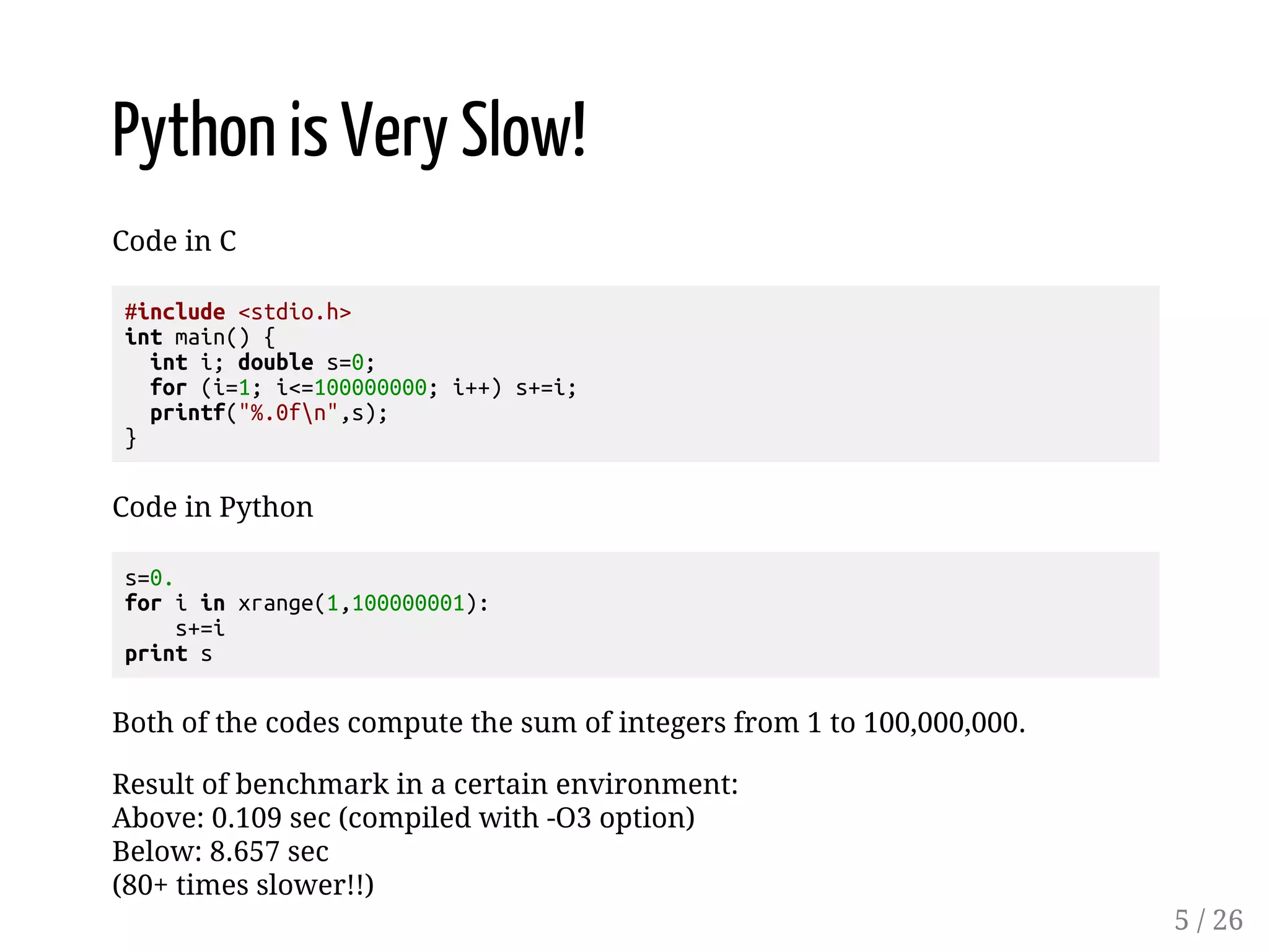
Highlighting Python's inefficiencies compared to C, demonstrating performance benchmarks, and discussing optimal coding practices for enhanced speed.
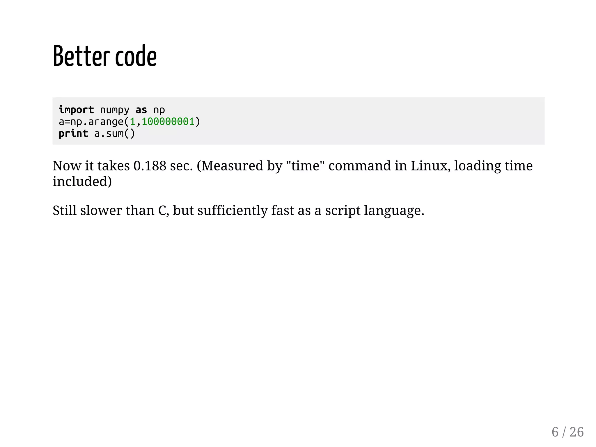
Guidelines for better performance in Python through NumPy, focusing on indexing, broadcasting, and memory management.
Examples of Boolean indexing in NumPy arrays, including comparisons and conditions, supplemented with a pandas DataFrame example.
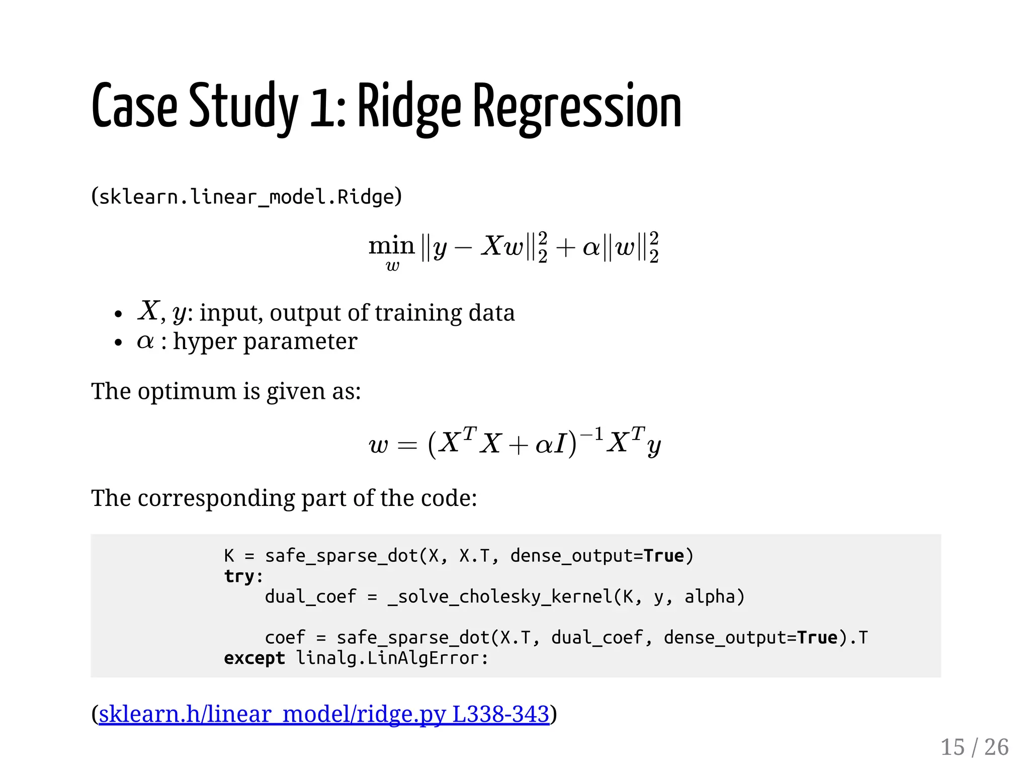
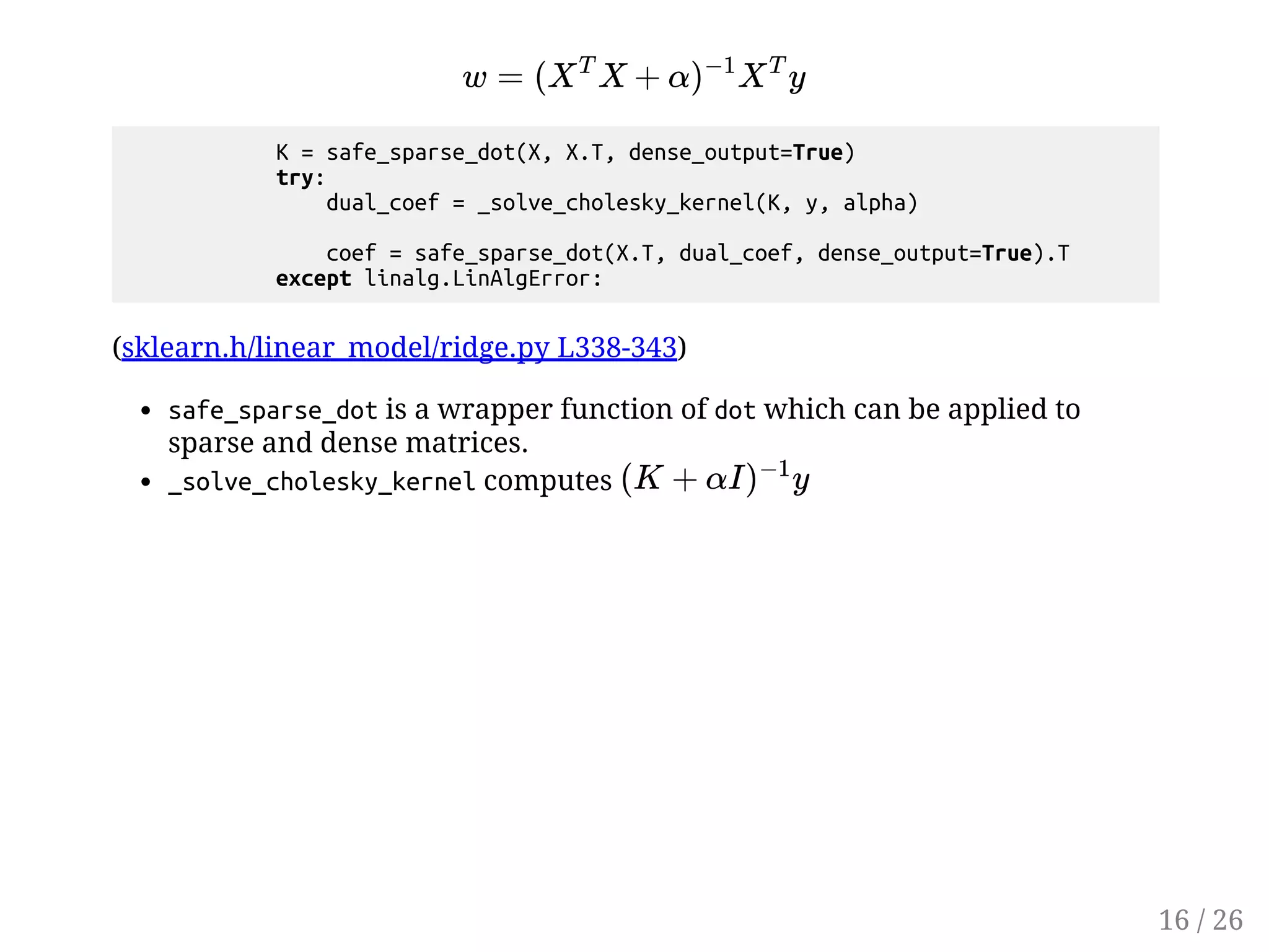
Explaining Ridge regression through scikit-learn, highlighting key equations, the role of matrices, and performance enhancements.
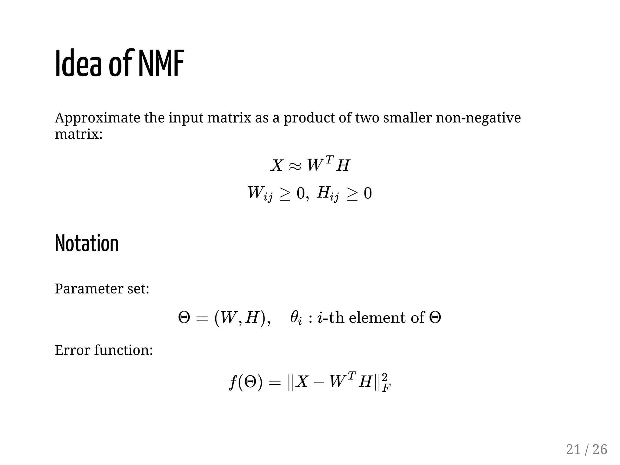
Introduction to NMF, the algorithm's approach to approximate matrices, and its application in tasks like face detection.
Summary of best practices using NumPy and references for further reading on scikit-learn and NumPy enhancements.