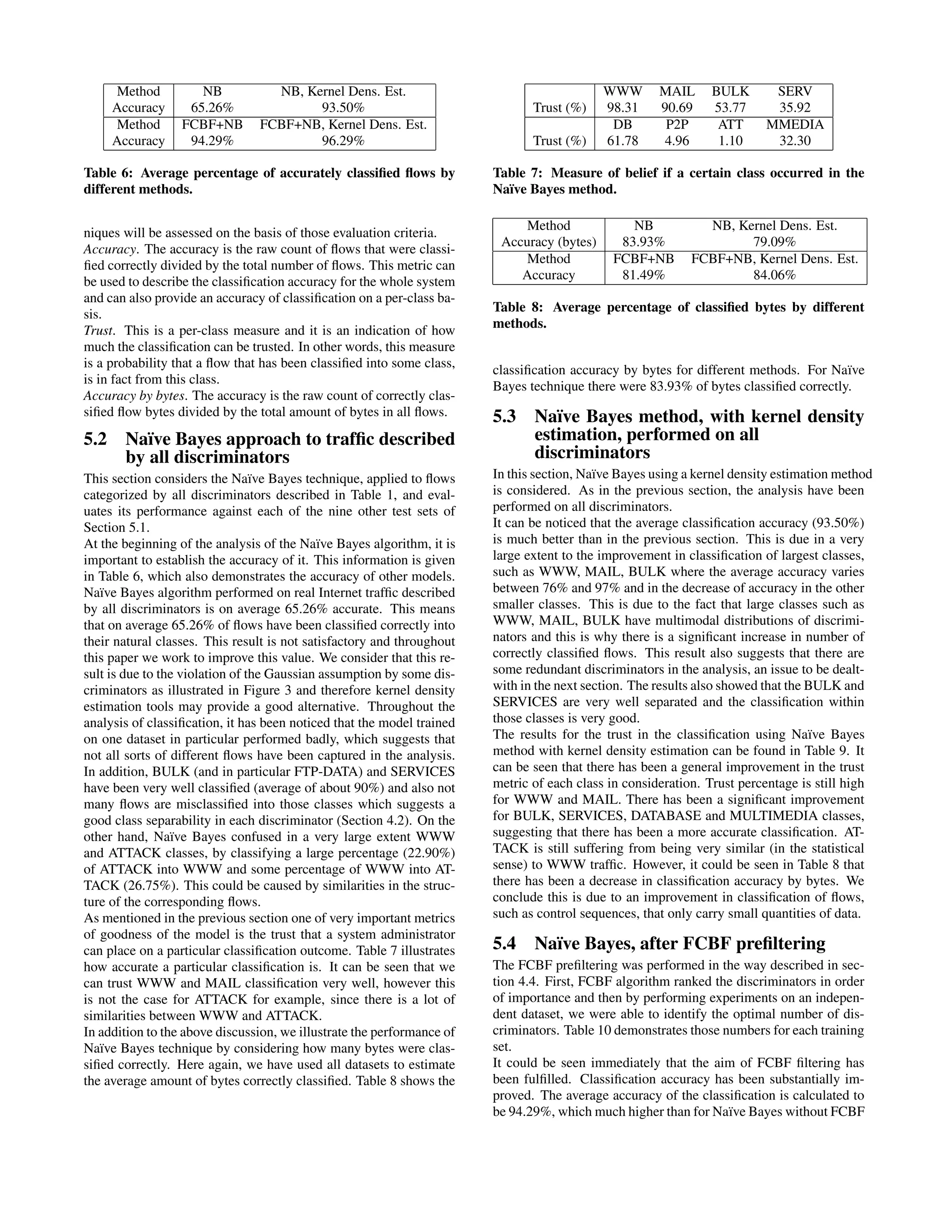
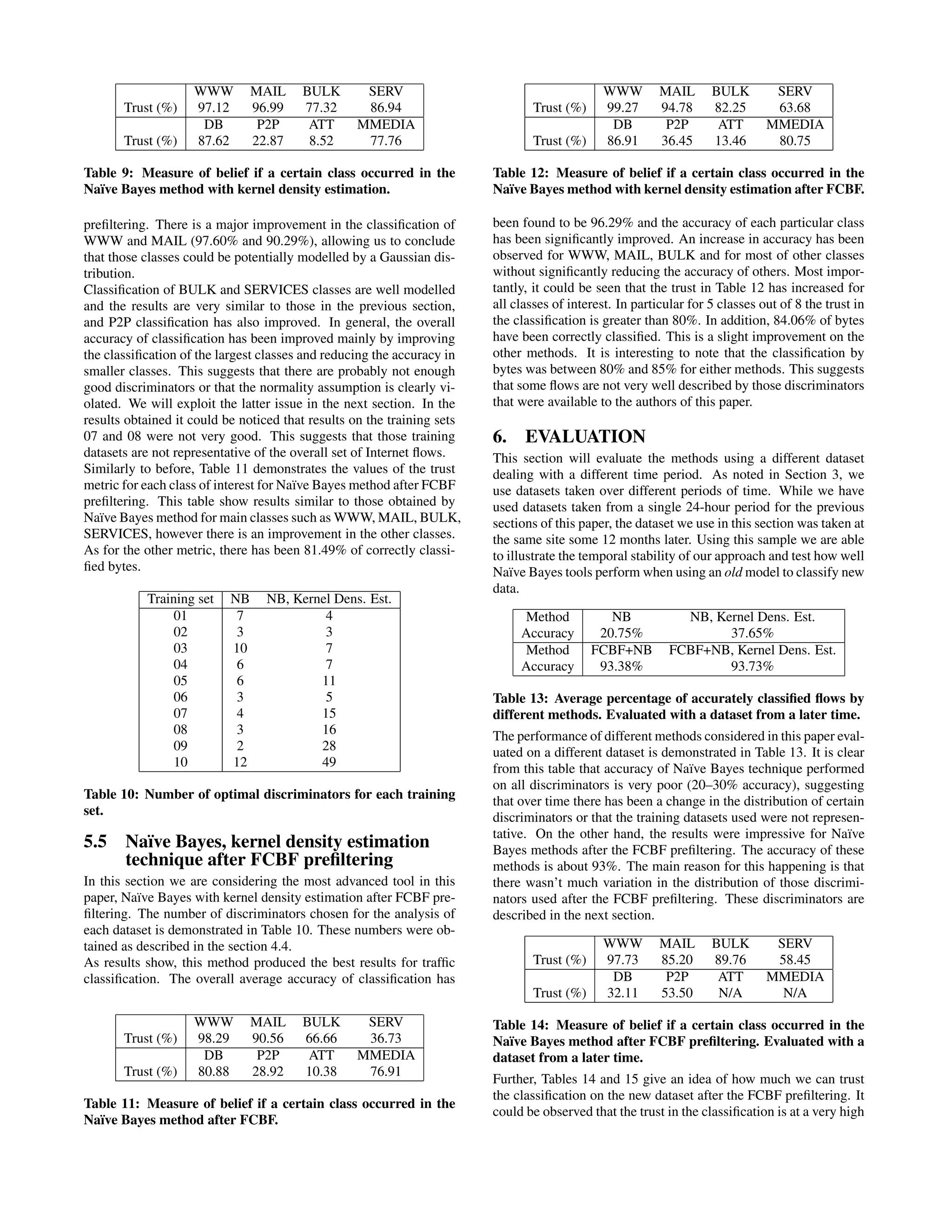
Internet Traffic Classification Using Bayesian Analysis Techniques

Internet Traffic Classification Using Bayesian Analysis Techniques

• 1.
  Internet Traffic ClassificationUsing Bayesian Analysis Techniques Andrew W. Moore ∗ University of Cambridge andrew.moore@cl.cam.ac.uk Denis Zuev † University of Oxford denis.zuev@maths.ox.ac.uk ABSTRACT Accurate traffic classification is of fundamental importance to nu- merous other network activities, from security monitoring to ac- counting, and from Quality of Service to providing operators with useful forecasts for long-term provisioning. We apply a Na¨ıve Bayes estimator to categorize traffic by application. Uniquely, our work capitalizes on hand-classified network data, using it as input to a supervised Na¨ıve Bayes estimator. In this paper we illustrate the high level of accuracy achievable with the Na¨ıve Bayes estima- tor. We further illustrate the improved accuracy of refined variants of this estimator. Our results indicate that with the simplest of Na¨ıve Bayes estima- tor we are able to achieve about 65% accuracy on per-flow clas- sification and with two powerful refinements we can improve this value to better than 95%; this is a vast improvement over traditional techniques that achieve 50–70%. While our technique uses train- ing data, with categories derived from packet-content, all of our training and testing was done using header-derived discriminators. We emphasize this as a powerful aspect of our approach: using samples of well-known traffic to allow the categorization of traffic using commonly-available information alone. Categories and Subject Descriptors I.5.1 [Computing Methodologies]: Pattern RecognitionModels; C.2.3 [Computer Communications-Networks]: Network Oper- ationsNetwork Monitoring; C.2.m [Computer Communications- Networks]: Miscellaneous General Terms Measurement, Algorithms Keywords Flow classification, Internet traffic, Traffic identification ∗Andrew Moore thanks the Intel Corporation for its generous sup- port of his research fellowship. †This work was completed when Denis Zuev was employed by In- tel Research, Cambridge. Permission to make digital or hard copies of all or part of this work for personal or classroom use is granted without fee provided that copies are not made or distributed for profit or commercial advantage and that copies bear this notice and the full citation on the first page. To copy otherwise, to republish, to post on servers or to redistribute to lists, requires prior specific permission and/or a fee. SIGMETRICS’05, June 6–10, 2005, Banff, Alberta, Canada. Copyright 2005 ACM 1-59593-022-1/05/0006 ...$5.00. 1. INTRODUCTION Accurate network traffic classification is fundamental to numer- ous network activities, from security monitoring to accounting, and from Quality of Service to providing operators with useful forecasts for long-term provisioning. Yet, classification schemes are difficult to operate correctly because the knowledge commonly available to the network, i.e. packet-headers, often does not contain sufficient information to allow for an accurate methodology. This leads to traditional techniques for traffic/flow classification that are often no-more accurate than 50–70% [1, 2, 3]. Our work uses supervised Machine-Learning to classify network traffic. Uniquely, we use data that has been hand-classified (based upon flow content) to one of a number of categories. Sets of data consisting of the (hand-assigned) category combined with descrip- tions of the classified flows (e.g., flow length, port numbers, time between consecutive flows) are used to train the classifier. We test our algorithm using data-sets consisting of only the object descrip- tions and then compare the predicted category with the actual cate- gory for each object. In the process of applying Na¨ıve Bayes we plan to provide insight into the behavior of this technique itself. We will illustrate the sen- sitivity of the Na¨ıve algorithm to its initial assumptions and we plan to demonstrate that the use of two techniques, one to break the Gaussian assumptions and the other to improve the quality of discriminators as input, lead to significant improvements in the ac- curacy of the Na¨ıve Bayes technique. We consider this paper illustrates the application of a powerful technique to a field different to those to which it has been previ- ously applied. We do this in anticipation of further work exploiting the techniques we describe as well as encouraging more research to bring new techniques to bear on this problem space. 1.1 Motivation As we noted earlier, the classification of traffic is an enabling func- tion for a variety of other applications and topics, including Quality of Service, security and intrusion-detection, monitoring. Further, Karagiannis et al. [4] identify an additional application of traffic categorization; they note that the growth or decline of particular traffic types can have a direct impact on social and political deci- sions, citing the perceived and actual growth of peer-2-peer net- works. Our work is made unique by the use of Internet traffic that has been manually classified. We use this traffic both for the training and testing of our algorithm. The data-set, along with the manual clas- sification process, is described elsewhere [5]. In contrast with the full-payload data used to enable precise classification, our method, once trained with data of a known classification, is able to be used to classify data for which only the TCP-headers are available.
• 2.
  Passively-collected packet-header traces,such as those performed by NLANR/MNA[7] and WAND[8], are commonly available and overcome issues of confidentiality and privacy. This widens the application of our procedure, enabling the categorization of traffic with a given accuracy and a known level of trust 1 . 2. RELATED WORK Due to its fundamental nature and its underpinning of many other techniques, the field of traffic classification has maintained contin- uous interest. For example, the most common technique for the identification of Internet network applications through traffic monitoring relies on the use of well known ports: an analysis of the headers of packets is used to identify traffic associated with a particular port and thus of a particular application [1, 2]. It is well known that such a pro- cess is likely to lead to inaccurate estimates of the amount of traffic carried by different applications given that specific protocols, such as HTTP, are frequently used to relay other types of traffic, e.g. a VLAN over HTTP. In addition, emerging services avoid the use of well known ports altogether, e.g. some peer-to-peer applications. Our work is presented in the light of these traditional classification techniques diminishing in effectiveness. Other authors that have noted the relationship between the class of traffic and its observed statistical properties include Paxson [6] who reports on the distribution of flow-bytes and flow-packets for a number of specific applications. While not considering the wider use of joint distributions for iden- tifying classes of traffic, Claffy [7] did observe that DNS traffic was clearly identifiable using the joint-distribution of flow-duration and the number of packets transferred. In an analysis of Internet chat systems, Dewes et al. [8] make ef- fective use of the packet-size profile of particular applications. The authors note that packets relevant to their studies tend towards a specific size-profile, limiting themselves to this profile allowed for a more precise selection of traffic relevant to their study. While not strictly classification, Floyd & Paxson [9] observe that simple (Poisson) models are unable to effectively capture some network characteristics. However, they did find a Poisson process could describe a number of events caused directly by the user; such as telnet packets within flows and connection arrivals for ftp-data. This paper is not the forum for a survey of the entire Machine Learning field. However, our approach may be contrasted with pre- vious work which attempts the classification of network traffic. We present a sample of such papers here. Roughan et al. [10] perform classification of traffic flows into a small number of classes suitable for Quality of Service applica- tions. The authors identify the set of useful features that will allow discrimination between classes. Limited by the amount of training data, the authors demonstrate the performance of nearest neighbor, LDA and QDA algorithms using several suitable features. In contrast, McGregor et al. [11] seek to identify traffic with sim- ilar observable properties and apply an untrained classifier to this problem. The untrained classifier has the advantage of identifying groups/classes of traffic with similar properties but does not directly assist in understanding what or why applications have been grouped this way. However, such a technique may be suitable for applying the first series of classification where the traffic is completely un- known and no previous classification has been previously applied. Soule et al. [12] attempt flow classification with a mind to iden- tifying membership among a smaller group of classes: the ele- phant flows — those of long-life and large data-content — and non- 1 Trust is defined in Section 5.1. elephant flows. Their method models flow histograms using Dirich- let Mixture Processes for random distributions which, combined with an inference procedure based on the Simulated Annealing Expectation Maximisation, allows estimation of flow-membership probability. The work of Hern´andex-Campos et al. [13] is intended to provide accurate information for their simulation work. To this end they use a hierarchical model represented as a dendrogram with each object representing the transfer of communications data between applications. A classification scheme based upon this representa- tion allows them to describe representative traffic patterns for input to the simulation work but does not intend to allow identification of the traffic itself. The field of security also uses ML techniques. However, they are attempting to do something fundamentally different from us where we are attempting to categories all traffic, intrusion-detection and related fields attempt to perform signature matching in order to identify intrusion or malicious software by it’s peculiar behavior among the continuum of otherwise legitimate activity. 3. EXPERIMENTAL SETUP Throughout this study we have used data collected by the high- performance network monitor described in [14]. We use its loss- limited, full-payload capture to disk providing time-stamps with resolution of better than 35 nanoseconds. We examine data for several different periods in time from one site on the Internet. This site is a research-facility host to about 1,000 users connected to the Internet via a full-duplex Gigabit Ethernet link. Full-duplex traffic on this connection was monitored for each traffic-set. The site we examined hosts several Biology-related facilities, col- lectively referred to as a Genome Campus. There are three insti- tutions on-site that employ about 1,000 researchers, administrators and technical staff. This campus is connected to the Internet via a full-duplex Gigabit Ethernet link. It was on this connection to the Internet that our monitor was placed. Traffic was monitored for each traffic-set consists of a full 24 hour, week-day period and for both link directions. 3.1 Objects and Discriminators As noted in Section 1, the application of a classification scheme requires the parameterizations of the objects to be classified. Using these parameters the classifier allocates an object to a class. Due to their ability to allow discrimination between classes, we refer to these object-describing parameters as discriminators. The fundamental object classified in our approach is a traffic-flow which is represented as a flow of one or more packets between a given pair of hosts. The flow is defined by a tuple consisting of the IP address of the pair of hosts, the protocol type (e.g., ICMP, TCP or UDP) and, in the case of UDP and TCP, the port numbers used by the two hosts. In the case of TCP, a flow has a finite duration defined by the semantics of the TCP protocol. For our work we limit ourselves to training and testing sets that consist only of TCP and are made-up of semantically 2 complete TCP connections. Our use of only complete TCP flows is a simplification that allows us to concentrate upon the classification process — rather than describe the mapping of datagram and partial-flows to objects. While not illustrated here, such a restriction is not necessary for the classifi- cation process. 2 Flows for which we see connection set-up (SYN-ACK packets) and tear-down (FIN-ACK packets).
• 3.
  Discriminator Flow duration TCP Port Packetinter-arrival time (mean, variance, ...) Payload size (mean, variance, ...) Effective Bandwidth based upon entropy[16] Fourier Transform of the packet inter-arrival time Table 1: Example discriminators describing each object and used as input for classification. Each of these discriminators is provided for both directions of the duplex traffic. Classification Example Application BULK ftp DATABASE postgres, sqlnet oracle, ingres INTERACTIVE ssh, klogin, rlogin, telnet MAIL imap, pop2/3, smtp SERVICES X11, dns, ident, ldap, ntp WWW www P2P KaZaA, BitTorrent, GnuTella ATTACK Internet worm and virus attacks GAMES Half-Life MULTIMEDIA Windows Media Player, Real Table 2: Network traffic allocated to each category. Each flow has a number of unique properties (e,g,. the source and destination ports 3 ), and a number of characteristics parameterizing its behavior — together these values form the input discriminators for our classification work. Table 1 gives a few examples drawn from the 248 per-flow discriminators that we use, the full list is given in [15]. 3.2 Traffic categories Fundamental to classification work is the idea of classes of traffic. Throughout this work we use classes of traffic defined as common groups of applications. Other users of classification may have both simpler definitions, e.g., Normal versus Malicious, or more com- plex definitions, e.g., the identification of specific applications or specific TCP implementations [17]. Adapted from Logg et al. [2], Table 2 lists the categories we use alongside a number of example applications. The application list given in this table is not defini- tive. A complete description along with the manual classification process is given in [5]. The use of such categories is also illustra- tive, allowing ready comparison with simpler port-only classifica- tion techniques. Importantly, while each flow is mapped to only one category, the characteristics of the traffic within each category are not necessar- ily unique. For example, the BULK category which is made up of ftp traffic consists of both the ftp control channel which trans- fers data in both directions, and the ftp data channel which consists of a simplex flow of data for each object transferred. The group- ing of applications into the categories we have given is largely an artificial, user-centric grouping and further serves to illustrate that such arbitrary clustering of only minimally-related traffic-types is possible within our scheme. 4. MACHINELEARNEDCLASSIFICATION Several methods exist for classifying data and all of them fall into two broad classes: deterministic and probabilistic (sometimes called 3 We explicitly do not use source or destination IP addresses as part of the classification process. This assists the site-independence of the trained model. hard and soft) classification. As the name suggests, determinis- tic classification assigns data points to one of mutually exclusive classes. This is done by considering some metric that defines the distance between data points and by defining the class boundaries. On the other hand, probabilistic classification methods classify data by assigning it with probabilities of belonging to each class of inter- est. For example after trying to classify an Internet flow using this method, it could be observed that with a probability of 0.8 this flow belongs to the MAIL class, with probability 0.1 to WWW class and with probability 0.1 to BULK class. Class assignment is done by considering the class with the largest probability. In the example, the flow will then be assigned to the MAIL class. We believe that our approach using the probabilistic classification of the Internet traffic is suitable because of the following reasons: • The method can identify similar characteristics of flows after their probabilistic class assignment. As an example, a flow classified with probability 0.8 in WWW and with probability 0.2 in BULK could represent a file-download tunnelled over the HTTP protocol. • The underlying statistical method is tractable and well docu- mented and understood. • The method is robust to measurement error. • The method allows for supervised training with pre-classified traffic. • The method can identify similar characteristics of flows after their probabilistic class assignment. • The method provides a mechanism for quantifying the class assignment probabilities. These in turn can warn the user of the declining accuracy of the model and/or indicate change in the network traffic or the introduction of new applications and protocols. In particular, this is a way of identifying when the model requires retraining. • Finally, ideally, the method is available in a number of com- monly available implementations. 4.1 Analysis Tools Research in the theory of machine learning has been developed for several years and there is a variety of different methods, each devel- oped to solve a particular problem in a certain area of science. Ex- amples illustrating the use of Bayes tools in various fields include text recognition, medical sciences and in astronomy (e.g., [18, 19, 20]). This paper considers Na¨ıve Bayes method, which as the name sug- gests is the simplest technique that could be applied to the problem in consideration. Results for this method will be demonstrated fur- ther in this paper. In addition to this, we consider a refinement of Na¨ıve Bayes method that improves the overall accuracy using ker- nel density estimation theory. As mentioned in the previous section, we will also consider a very promising method of feature selection and redundancy reduction, Fast Correlation-Based Filter (FCBF) described in [21]. 4.2 Na¨ıve Bayesian Classifier In this section we will remind the reader about Bayes methods and explain the theory of the Na¨ıve Bayes classifier. Additional infor- mation on Na¨ıve Bayes technique could be found in [22]. Consider a data sample x = (x1, . . . , xn) which is a realization of X = {X1, . . . , Xn} such that each random variable Xi is de- scribed by m attributes {A1, . . . , Am} (referred to as discrimina- tors) that can take numeric or discrete values. Xi = A (i) 1 , . . . . . . , A (i) m T is then a random vector. As an example, for Internet
• 4.
  traffic, A (i) j mayrepresent the mean inter-arrival time of packets in the flow i. Assume now that there are k known classes of interest. Let C = {c1, . . . , ck} represent the set of all known classes. For each ob- served instance xi in x, there is a known mapping C : x → C representing the membership of instance xi to a particular class of interest. The notation C(xi) = cj stands for “the instance xi be- longs to the class cj”. Bayesian statistical conclusions about the class cj of an unobserved flow y are based on probability conditional on observing the flow y. This is called the posterior probability and is denoted by p(cj | y). The celebrated Bayes rules gives a way of calculating this value: p(cj | y) = p(cj)f(y | cj) cj p(cj)f(y | cj) (1) where p(cj) denotes the probability of obtaining class cj indepen- dently of the observed data (prior distribution), f(y | cj) is the distribution function (or the probability of y given cj) and the de- nominator acts as a normalizing constant. The goal of the supervised Bayes classification problem is to es- timate f(y | cj), j = 1, . . . , k given some training set x. To do that, Na¨ıve Bayes makes certain assumptions on f(· | cj) such as independence of Ai’s and the standard Gaussian behavior of them. The problem is then reduced to simply estimating the parameters of the Gaussian distribution and the prior probabilities of cj’s. In fact, Na¨ıve Bayes is also capable of dealing with discrete random discriminators, which could represent the state of some flag of a flow, by treating them independently and using the frequencies of occurrences to estimate f(· | cj), j = 1, . . . , k. In reality, independence and normality assumptions are flawed for the problem in consideration: • Different discriminators are clearly not independent. An ex- ample is packet-header size statistics. The TCP header size may vary directly in proportion with the total packet-length no matter what the other characteristics of the traffic might be. • Assumption of the normality of discriminators is also inac- curate. Notable problems arise when the real distribution is multi-modal. This situation may suggest that the class in consideration is too broad (WWW for example,) or that we should consider another distribution for data analysis. This latter method is explored in particular in Section 4.3. Although these assumptions are not realistic, Na¨ıve Bayes has been shown to work better than more-complex methods and cope with complex situations [22]. Additionally, we emphasis the advantages of using the simplest of computational methods in order to ensure the process is tractable in time. This idea of Na¨ıve Bayes technique can be illustrated by assuming simply that m = 1 and k = 2 (there is only one discriminator of Xi and there are two classes of interest, c1, c2). Figure 1 demonstrates distribution of data in this probabilistic setup: data from class c1 is distributed normally with mean 3 and variance 1, whereas data from class c2 is distributed normally with mean 10 and variance 2. From the picture, it is clear that the error of misclassification is re- duced by minimizing the intersection area of the two distributions. In practice, a training sample x = (x1, . . . , xn) in which we know that nc1 instances belong to c1 and nc2 instances belong to c2 (nc1 + nc2 = n) allows estimating the prior probabilities of the classes cj’s by: p(c1) = nc1 n , (2) p(c2) = nc2 n . (3) 0 5 10 15 20 0.00.10.20.30.4 x denisity Figure 1: Example of two normal distributions N(3,1) and N(10,2). As described above, the method assumes Gaussian distribution for f(· | cj), j = 1, . . . , k, fA1|c1 (x; µ1, σ2 1) = 1 2πσ2 1 e − (x−µ1)2 2σ2 1 (4) and fA1|c2 (x; µ2, σ2 2) = 1 2πσ2 2 e − (x−µ2)2 2σ2 2 . (5) As the information about the classes is given, the distribution pa- rameters µ1, µ2, σ2 1, σ2 2 are estimated by appropriate maximum likelihood estimators: ˆµ1 = xi:C(xi)=c1 xi nc1 , ˆµ2 = xi:C(xi)=c2 xi nc2 , ˆσ2 1 = xi:C(xi)=c1 (xi−ˆµ1)2 nc1 −1 , ˆσ2 2 = xi:C(xi)=c2 (xi−ˆµ2)2 nc2 −1 . Given a flow y to be classified, its posterior probability of class membership is given by p(ci | y) = fA1|ci (y; ˆµi, ˆσ2 i ) × p(ci) N , (6) i = 1, 2 and N is a normalizing constant. 4 4.3 Na¨ıve Bayes: Kernel Estimation The Na¨ıve Bayes Kernel estimation method is a generalization of Na¨ıve Bayes and it addresses the problem of approximating every discriminator by a Gaussian distribution as described in the previ- ous section. 4 Strictly speaking, equation (6) is not really correct because fA1|ci (y; ˆµi, ˆσ2 i ) is a density function, rather than a probability. In fact, the quantity of interest is the probability of Y = y, given cj, which is 0 as Y is a continuous random variable. Instead, we are interested in P(Y ∈ (y, y + )) ≈ fA1|ci (y; ˆµi, ˆσ2 i ) × , by the Mean Value Theorem. is canceled by the denominator and therefore (6) is obtained.
• 5.
  Na¨ıve Bayes KernelEstimation is similar to Na¨ıve Bayes method algorithmically and the only difference arises in estimating f(· | cj), j = 1, . . . , k. Whereas Na¨ıve Bayes estimated f(· | cj), j = 1, . . . , k by fitting a Gaussian distribution over the data, Kernel Estimation, as the name suggests, uses kernel estimation methods, i.e. the estimate of the real density f(· | cj) is given by ˆf(t | cj) = 1 ncj h xi:C(xi)=cj K t − xi h , (7) where h is called the kernel bandwidth and K(t) is any kernel, where kernel is defined as any non-negative function (although it is possible to generalise) such that ∞ −∞ K(t)dt = 1. Examples of such distributions are: uniform distribution (K(t) = 1 2 I(|t| ≤ 1)) which generates a histogram to approximate f(·), Gaussian distri- bution (K(t) = 1√ 2π exp (−t2 /2)) and many others [23]. Na¨ıve Bayes kernel estimation procedure will use Gaussian density as the kernel for the analysis, party because it is Gaussian density has de- sirable smoothness properties. Figure 2 illustrates how an estimate of the density f(·) is constructed. Assume that some sample of data points has been collected. These points are represented by crosses on the x-axis. For each data point a Gaussian distribution centered on this point is fitted. A summation of those functions gives an estimate of the real density of the data distribution. -10 -5 0 5 10 DensityEstimate Data x Construction of Kernel Density Function Figure 2: An illustration of how the estimate of the distribution is constructed. The selection of the statistical bandwidth, as defined in the previous paragraph, plays an important role in the accuracy of the model and some nice theoretical properties are mentioned in [24]. Bandwidth has an effect on the accuracy of approximation, which is very often measured by Mean Integrated Squared Error, which is defined as: MISE( ˆf) = E ˆf(t) − f(t) 2 dt .5 (8) Figure 3 illustrates different ways of estimating the density. For the purpose of this paper, the value of the parameter h is taken to be the default value of the WEKA software suite used to perform calculations in this paper. All tools used in this paper are described in section 5. In [24], it is shown that the Kernel Estimation method performs much better in situations when the normality assumption is strongly 5 It is important to understand that ˆf(t) is in fact a random function since data observations are random. It therefore makes sense to take the expectation in (8). Data Density 60 80 100 120 140 0.000.010.020.03 Figure 3: Different estimators of the density that generated the data. The black line represents the Gaussian density whose pa- rameters were estimated from the data, the two dashed lines represent the kernel estimated density with two different val- ues of the bandwidth. NA¨IVE BAYES KERNEL Operation Time Space Time Space Train on n cases O(nm) O(m) O(nm) O(nm) Test on q cases O(qm) O(qnm) Table 3: Algorithmic complexity for Na¨ıve Bayes and Kernel Estimation method, given n training instances and m discrimi- nators. violated, but on the other hand it performs just as well when the data is Gaussian as long as there are enough instances. There are however computational issues related to the Kernel Esti- mation method. When computing f(. | cj) to classify an unknown instance, Na¨ıve Bayes has to evaluate the Gaussian distribution only once whereas Kernel Estimation must perform n evaluations. Table 3 contrasts the computational and memory requirements for the two methods. 4.4 Discriminator selection and dimension reduction Discriminator selection and dimension reduction plays a very im- portant role in Machine Learning by acting as a preprocessing step, removing redundant and irrelevant discriminators. As described in [22], the prediction accuracy of the Na¨ıve Bayes algorithm suf- fers from the presence of irrelevant and redundant attributes. The ability to identify the most important discriminators of the Inter- net traffic is useful not only because the results will reveal what discriminators are best for traffic classification, but also because classification accuracy can be improved and, a reduction in number of flow discriminators is computationally attractive. Before going into the theory, it is important to define what is meant by irrelevant and redundant discriminators. Definition 1: A discriminator is said to be irrelevant if it carries no information about different classes of interest. This discriminator has no discriminative power. For example, a discriminator may take only a single value and, on that basis, no classification could be made. Definition 2: A discriminator is said to be redundant if it is highly correlated with another discriminator. The reason for removing redundant discriminators is supported by the fact that redundant
• 6.
  discriminators either worsenthe accuracy or increase over-fitting. Consider a discriminator that is a not a very good one and assume that there is another discriminator that is very highly correlated to the first one. Using Na¨ıve Bayes technique, considering two dis- criminators is equivalent to putting a greater weight on one of the them without considering their relative merits. There exist two different approaches to discriminator selection, namely the filter and the wrapper methods. Filter methods use the characteristics of the training data to determine the relevance and importance of certain discriminators to the classification problem. For example, a measure of relevance could be the degree of correla- tion between discriminators and the class, or some measure of sepa- ration of classes based on the discriminator in consideration. On the other hand, wrapper methods make use of the results of a particular classifier (e.g. Na¨ıve Bayes) to build the optimal set by evaluating the results of the classifier on a test set for different combinations of discriminators. By re-iterating the algorithm, the user can iden- tify the optimal set of discriminators that are suited for a particular classification method (e.g. Na¨ıve Bayes). One such method would be the “forward selection” method, where one starts with no at- tributes and progressively adds one attribute after the other, check- ing the outcome after each additional attribute. A second example is “backward elimination”, where one starts with the full set of dis- criminators to work “backward” by eliminating discriminators one after the other. The main drawback of this method is that it is very computationally expensive, particularly in high dimensions as one needs to try each combination of a number of different discrimina- tors. In this paper, we will be using Fast Correlation-Based Filter (FCBF), described in [21], as well as a variation of a wrapper method in determining the value of the threshold (described later in this Sec- tion). The FCBF filter method performs very well in improving the performance of Na¨ıve Bayes when contrasted with other related techniques [21]. According to [21], a discriminator is good if it is relevant to the class concept but it is not redundant to any of the other relevant features. In FCBF, goodness of a discriminator is measured by its correlation with the class and other good attributes. That attribute becomes good if it is highly correlated with the class, yet not cor- related with any other good attributes. The correlation measure used in FCBF is based on the entropy of a random variable — a measure of uncertainty. The entropy of a discrete random variable X taking values in {x1, . . . , xn} is given by H(X) = − xi p(xi) log2 p(xi), (9) and the entropy of a discrete random variable X given Y is given by H(X | Y ) = − yj p(yj) xi p(xi | yj) log2 p(xi | yj), (10) where p(xi) = P[X = xi], p(yj) = P[Y = yj] and p(xj | xj) = P[X = xi | Y = yj]. Similarly, the information gain, [25], is expressed as IG(X | Y ) = H(X) − H(X | Y ). (11) Information gain (11) is a measure of correlation between two dis- criminators. In practice, the discriminator X is considered to be more correlated to the discriminator Y , than to discriminator Z, if IG(X | Y ) > IG(X | Z). Moreover, [21] show that the informa- tion gain is symmetric for random variables X and Y . Using equations (9) and (11), symmetrical uncertainty is defined in the following way: SU(X, Y ) = 2 IG(X | Y ) H(X) + H(Y ) . (12) Symmetrical uncertainty (12) takes values in [0, 1], where the value 1 means that the knowledge of discriminator values induces the value of the other, while 0 suggests that attributes X and Y are in- dependent. By this point, Equation (12) has only been defined for nominal values 6 , therefore FCBF continuous discriminators dis- crete before the core analysis [21]. The FCFB algorithm selects good discriminators via a two stage process by: • identifying the relevance of a discriminator, • identifying the redundancy of a feature with respect to other discriminators. To describe these concepts mathematically, let C denote the ran- dom variable of traffic classes taking values in C. Further, let SUi,c and SUi,j denote the value of the symmetric uncertainty between Ai and C and between Ai and Aj respectively. A discriminator Ai is believed to be relevant if SUi,c ≥ δ, where δ is some threshold value to be determined by the user. Identification of redundancy is often done by computing the pair- wise cross correlations between discriminators. However, [21] note that this method is quite computationally expensive and so the solu- tion they propose considers SU values, because symmetrical uncer- tainty captures pairwise cross correlation information. As a result, FCBF works in the following way. Initially, SUj,c, 1 ≤ j ≤ m are calculated and discriminators are ordered in descending order according to the values of SU. A set S is created, containing Ajs that satisfy SUj,c ≥ δ. Then, the discriminator with the largest SUj,c (call it Ap) is compared to SUj,q, where Aq ∈ S Ap. If SUj,q ≥ SUp,c, the discriminator Aq is considered redundant and is therefore removed from S. The procedure is repeated for all Ap’s in S. The complexity of this algorithm is O(nm log m). At last, the question arises as to how to determine the optimal value of the threshold δ. To overcome this difficulty, we use a wrapper method based upon Na¨ıve Bayes algorithm, i.e. computational re- sults of the Na¨ıve Bayes algorithm will be used to estimate the opti- mal value of the threshold. This approach has the goal of maximiz- ing some measure of accuracy (e.g., percentage of correctly classi- fied flows). The advantage of this approach is that it is less com- putationally expensive that the “forward selection” or “backward elimination”, since only m cases are needed to be checked com- pared to 2m − 1. In addition, this method specifically improves the predictive capability of Na¨ıve Bayes technique alone, rather than trying to improving the accuracy of all available Machine Learning tools. The following algorithm is used to identify the best number of dis- criminators to be used for a particular training set. • Rank all discriminators in order of importance as calculated by the FCBF method. • The goal is the to determine how many of the most impor- tant discriminators to choose. To do that an independent set of test data is chosen and it is used to evaluate the perfor- mance of Na¨ıve Bayes classifier trained on different number of discriminators. • For n from 1 to m, train Na¨ıve Bayes on the training set with n discriminators and evaluate the resulting classifier on the test set. 6 Although it is possible to define it for continuous random vari- ables; the estimation of probabilities is then much harder.
• 7.
  Total Flows WWWMAIL BULK SERV DB 377526 328091 28567 11539 2099 2648 INT P2P ATTACK MMEDIA GAMES 110 2094 1793 1152 8 Table 4: Data statistics (number of flows). 15 45 75 30 60 90 00:00 12:00 18:00 Mbps Time (GMT)06:00 01 02 03 04 05 06 07 08 09 10 Block Number Figure 4: Heuristic illustration of how data blocks were ob- tained. The line represents the instantaneous bandwidth re- quirements during the day, while the dark regions represent the data blocks that are used in the analysis of the accuracy of Na¨ıve Bayes methods. • Choose n such that it maximizes the classification accuracy. It is can be seen that this algorithm uses both filter and wrapper methods to determine the optimal set of discriminators. 5. RESULTS 5.1 Setup Analysis Data This section describes how the data for training and testing was obtained, as well as the characteristics, trends of this data. In the analysis of the accuracy of different methods in consideration, ten different data sets were chosen. An eleventh dataset is separately described and used in Section 6. In order to construct a set of flows, the day trace was split into ten blocks of approximately 1680 sec- onds (28 min) each. In order to provide a wider sample of mixing across the day, the start of each sample was randomly selected, uni- formly over the whole day trace. Figure 4 illustrates heuristically our technique. It can be seen from Table 4 that there are different number of flows in each data block, due to a higher density of traf- fic during each block of 28 minutes. Since time statistics of flows are present in the analysis, we consider it important to keep a fixed time window when selecting flows. Table 4 contains information about the structure of the dataset (a sum of flows in each of datasets 01 through 10, etc.) that is being used in the evaluation of different methods. While the table sum- marizes the break-down, it is clear from these numbers that for the INTERACTIVE and GAMES classes there is not enough data to make the accurate analysis of these classes tractable. The accuracy of each method is evaluated by training the classifier using one data-set and then testing it against the remaining (9) data sets. This process cycle of training with one data-set and training against the other data-sets is repeated once for each data-set. The gross statistics for accuracy and trust are accumulated for all ten evaluations. Using the group of tests against data-sets each taken at Memory # of discriminators max # of instances 32M 132 6500–7000 64M 132 13000–13500 128M 132 25000 32M 265 3000–3500 64M 265 6500–7000 128M 265 12000–12500 256M 265 24500–25000 Table 5: Memory usage by WEKA. a different period over the day allows us to draw conclusions based upon data drawn over the whole 24-hour period. Additionally we can gain insight about the average of results for each technique. Analysis Tools In this work, analysis with the Na¨ıve Bayes, kernel density esti- mation and FCBF methods were performed using version 3.4 of the WEKA software suite [22]. WEKA, written in the Java lan- guage, allows tracking of its memory footprint. Table 5 illustrates the memory constraints relating these to both the number of objects over which to construct the model and the number of discrimina- tors used to describe each object. Numbers in Table 5 should be interpreted in the following way. Given X amount of memory and Y number of discriminators, this table shows an estimate of the maximum number of instances that can be loaded into the WEKA software. Due to its simplicity, the Na¨ıve Bayes method is quite fast, com- pared to other methods. Figure 5 shows how much time it needs to build a model on the training set of 24863 flows and test it against a test set of 23801 flows in relation to the number of discriminators. It can be seen that the line obtained is almost linear and in fact some variation in the linearity is due to the complexity of the discrimi- nators in use (by complexity we mean whether the discriminator is discrete or continuous). 0 50 100 150 200 050100150200250300 Number of discriminators Time(s) Figure 5: Time taken to build a model on a training set (24863 flows) and test it against the test set (23801 flows) in relation to the number of discriminators in consideration. Evaluation Criteria The authors of this paper use two metrics to assess the performance of different techniques. In particular, refinements to those tech-
• 8.
  Method NB NB,Kernel Dens. Est. Accuracy 65.26% 93.50% Method FCBF+NB FCBF+NB, Kernel Dens. Est. Accuracy 94.29% 96.29% Table 6: Average percentage of accurately classified flows by different methods. niques will be assessed on the basis of those evaluation criteria. Accuracy. The accuracy is the raw count of flows that were classi- fied correctly divided by the total number of flows. This metric can be used to describe the classification accuracy for the whole system and can also provide an accuracy of classification on a per-class ba- sis. Trust. This is a per-class measure and it is an indication of how much the classification can be trusted. In other words, this measure is a probability that a flow that has been classified into some class, is in fact from this class. Accuracy by bytes. The accuracy is the raw count of correctly clas- sified flow bytes divided by the total amount of bytes in all flows. 5.2 Na¨ıve Bayes approach to traffic described by all discriminators This section considers the Na¨ıve Bayes technique, applied to flows categorized by all discriminators described in Table 1, and eval- uates its performance against each of the nine other test sets of Section 5.1. At the beginning of the analysis of the Na¨ıve Bayes algorithm, it is important to establish the accuracy of it. This information is given in Table 6, which also demonstrates the accuracy of other models. Na¨ıve Bayes algorithm performed on real Internet traffic described by all discriminators is on average 65.26% accurate. This means that on average 65.26% of flows have been classified correctly into their natural classes. This result is not satisfactory and throughout this paper we work to improve this value. We consider that this re- sult is due to the violation of the Gaussian assumption by some dis- criminators as illustrated in Figure 3 and therefore kernel density estimation tools may provide a good alternative. Throughout the analysis of classification, it has been noticed that the model trained on one dataset in particular performed badly, which suggests that not all sorts of different flows have been captured in the analysis. In addition, BULK (and in particular FTP-DATA) and SERVICES have been very well classified (average of about 90%) and also not many flows are misclassified into those classes which suggests a good class separability in each discriminator (Section 4.2). On the other hand, Na¨ıve Bayes confused in a very large extent WWW and ATTACK classes, by classifying a large percentage (22.90%) of ATTACK into WWW and some percentage of WWW into AT- TACK (26.75%). This could be caused by similarities in the struc- ture of the corresponding flows. As mentioned in the previous section one of very important metrics of goodness of the model is the trust that a system administrator can place on a particular classification outcome. Table 7 illustrates how accurate a particular classification is. It can be seen that we can trust WWW and MAIL classification very well, however this is not the case for ATTACK for example, since there is a lot of similarities between WWW and ATTACK. In addition to the above discussion, we illustrate the performance of Na¨ıve Bayes technique by considering how many bytes were clas- sified correctly. Here again, we have used all datasets to estimate the average amount of bytes correctly classified. Table 8 shows the WWW MAIL BULK SERV Trust (%) 98.31 90.69 53.77 35.92 DB P2P ATT MMEDIA Trust (%) 61.78 4.96 1.10 32.30 Table 7: Measure of belief if a certain class occurred in the Na¨ıve Bayes method. Method NB NB, Kernel Dens. Est. Accuracy (bytes) 83.93% 79.09% Method FCBF+NB FCBF+NB, Kernel Dens. Est. Accuracy 81.49% 84.06% Table 8: Average percentage of classified bytes by different methods. classification accuracy by bytes for different methods. For Na¨ıve Bayes technique there were 83.93% of bytes classified correctly. 5.3 Na¨ıve Bayes method, with kernel density estimation, performed on all discriminators In this section, Na¨ıve Bayes using a kernel density estimation method is considered. As in the previous section, the analysis have been performed on all discriminators. It can be noticed that the average classification accuracy (93.50%) is much better than in the previous section. This is due in a very large extent to the improvement in classification of largest classes, such as WWW, MAIL, BULK where the average accuracy varies between 76% and 97% and in the decrease of accuracy in the other smaller classes. This is due to the fact that large classes such as WWW, MAIL, BULK have multimodal distributions of discrimi- nators and this is why there is a significant increase in number of correctly classified flows. This result also suggests that there are some redundant discriminators in the analysis, an issue to be dealt- with in the next section. The results also showed that the BULK and SERVICES are very well separated and the classification within those classes is very good. The results for the trust in the classification using Na¨ıve Bayes method with kernel density estimation can be found in Table 9. It can be seen that there has been a general improvement in the trust metric of each class in consideration. Trust percentage is still high for WWW and MAIL. There has been a significant improvement for BULK, SERVICES, DATABASE and MULTIMEDIA classes, suggesting that there has been a more accurate classification. AT- TACK is still suffering from being very similar (in the statistical sense) to WWW traffic. However, it could be seen in Table 8 that there has been a decrease in classification accuracy by bytes. We conclude this is due to an improvement in classification of flows, such as control sequences, that only carry small quantities of data. 5.4 Na¨ıve Bayes, after FCBF prefiltering The FCBF prefiltering was performed in the way described in sec- tion 4.4. First, FCBF algorithm ranked the discriminators in order of importance and then by performing experiments on an indepen- dent dataset, we were able to identify the optimal number of dis- criminators. Table 10 demonstrates those numbers for each training set. It could be seen immediately that the aim of FCBF filtering has been fulfilled. Classification accuracy has been substantially im- proved. The average accuracy of the classification is calculated to be 94.29%, which much higher than for Na¨ıve Bayes without FCBF
• 9.
  WWW MAIL BULKSERV Trust (%) 97.12 96.99 77.32 86.94 DB P2P ATT MMEDIA Trust (%) 87.62 22.87 8.52 77.76 Table 9: Measure of belief if a certain class occurred in the Na¨ıve Bayes method with kernel density estimation. prefiltering. There is a major improvement in the classification of WWW and MAIL (97.60% and 90.29%), allowing us to conclude that those classes could be potentially modelled by a Gaussian dis- tribution. Classification of BULK and SERVICES classes are well modelled and the results are very similar to those in the previous section, and P2P classification has also improved. In general, the overall accuracy of classification has been improved mainly by improving the classification of the largest classes and reducing the accuracy in smaller classes. This suggests that there are probably not enough good discriminators or that the normality assumption is clearly vi- olated. We will exploit the latter issue in the next section. In the results obtained it could be noticed that results on the training sets 07 and 08 were not very good. This suggests that those training datasets are not representative of the overall set of Internet flows. Similarly to before, Table 11 demonstrates the values of the trust metric for each class of interest for Na¨ıve Bayes method after FCBF prefiltering. This table show results similar to those obtained by Na¨ıve Bayes method for main classes such as WWW, MAIL, BULK, SERVICES, however there is an improvement in the other classes. As for the other metric, there has been 81.49% of correctly classi- fied bytes. Training set NB NB, Kernel Dens. Est. 01 7 4 02 3 3 03 10 7 04 6 7 05 6 11 06 3 5 07 4 15 08 3 16 09 2 28 10 12 49 Table 10: Number of optimal discriminators for each training set. 5.5 Na¨ıve Bayes, kernel density estimation technique after FCBF prefiltering In this section we are considering the most advanced tool in this paper, Na¨ıve Bayes with kernel density estimation after FCBF pre- filtering. The number of discriminators chosen for the analysis of each dataset is demonstrated in Table 10. These numbers were ob- tained as described in the section 4.4. As results show, this method produced the best results for traffic classification. The overall average accuracy of classification has WWW MAIL BULK SERV Trust (%) 98.29 90.56 66.66 36.73 DB P2P ATT MMEDIA Trust (%) 80.88 28.92 10.38 76.91 Table 11: Measure of belief if a certain class occurred in the Na¨ıve Bayes method after FCBF. WWW MAIL BULK SERV Trust (%) 99.27 94.78 82.25 63.68 DB P2P ATT MMEDIA Trust (%) 86.91 36.45 13.46 80.75 Table 12: Measure of belief if a certain class occurred in the Na¨ıve Bayes method with kernel density estimation after FCBF. been found to be 96.29% and the accuracy of each particular class has been significantly improved. An increase in accuracy has been observed for WWW, MAIL, BULK and for most of other classes without significantly reducing the accuracy of others. Most impor- tantly, it could be seen that the trust in Table 12 has increased for all classes of interest. In particular for 5 classes out of 8 the trust in the classification is greater than 80%. In addition, 84.06% of bytes have been correctly classified. This is a slight improvement on the other methods. It is interesting to note that the classification by bytes was between 80% and 85% for either methods. This suggests that some flows are not very well described by those discriminators that were available to the authors of this paper. 6. EVALUATION This section will evaluate the methods using a different dataset dealing with a different time period. As noted in Section 3, we use datasets taken over different periods of time. While we have used datasets taken from a single 24-hour period for the previous sections of this paper, the dataset we use in this section was taken at the same site some 12 months later. Using this sample we are able to illustrate the temporal stability of our approach and test how well Na¨ıve Bayes tools perform when using an old model to classify new data. Method NB NB, Kernel Dens. Est. Accuracy 20.75% 37.65% Method FCBF+NB FCBF+NB, Kernel Dens. Est. Accuracy 93.38% 93.73% Table 13: Average percentage of accurately classified flows by different methods. Evaluated with a dataset from a later time. The performance of different methods considered in this paper eval- uated on a different dataset is demonstrated in Table 13. It is clear from this table that accuracy of Na¨ıve Bayes technique performed on all discriminators is very poor (20–30% accuracy), suggesting that over time there has been a change in the distribution of certain discriminators or that the training datasets used were not represen- tative. On the other hand, the results were impressive for Na¨ıve Bayes methods after the FCBF prefiltering. The accuracy of these methods is about 93%. The main reason for this happening is that there wasn’t much variation in the distribution of those discrimi- nators used after the FCBF prefiltering. These discriminators are described in the next section. WWW MAIL BULK SERV Trust (%) 97.73 85.20 89.76 58.45 DB P2P ATT MMEDIA Trust (%) 32.11 53.50 N/A N/A Table 14: Measure of belief if a certain class occurred in the Na¨ıve Bayes method after FCBF prefiltering. Evaluated with a dataset from a later time. Further, Tables 14 and 15 give an idea of how much we can trust the classification on the new dataset after the FCBF prefiltering. It could be observed that the trust in the classification is at a very high
• 10.
  level of morethan 87% in 3 classes out of 6. It also is worth noting that the P2P traffic has been classified better than in previous sec- tions implying that the model we have trained previously is getting more accurate over time. WWW MAIL BULK SERV Trust (%) 98.06 87.54 90.03 44.54 DB P2P ATT MMEDIA Trust (%) 68.63 55.18 N/A N/A Table 15: Measure of belief if a certain class occurred in the Na¨ıve Bayes, kernel density estimation method after FCBF pre- filtering. Evaluated with a dataset from a different time. 7. IDENTIFICATION OF IMPORTANT DISCRIMINATORS The refinement of our classification is impacted by the selection of the appropriate discriminator. Firstly, a good discriminator must provide good separation among the classes, thereby agreeing with the theory in Section 4. Secondly, the ideal discriminator provides a function for each class that can be well approximated by a Gaussian distribution. The example given in Figure 6 illustrates how the data is distributed for the discriminator: SACKs send from client to server. Clearly this distribution provides reasonable separation for the three classes shown and allows for a Gaussian distribution — important for Na¨ıve Bayes — to approximate at least two of them. 0 80 140 200 260 320 380 440 500 560 620 680 740 800 860 940 1000 SACKs sent from client to server BULK MAIL WWW 0 80 140 200 260 320 380 440 500 560 620 680 740 800 860 940 1000 SACKs sent from client to server BULK MAIL WWW Figure 6: Example histogram of SACKs send from client to server The FCBF used in Sections 5.4 and 5.5 allowed us to identify dis- criminators that provided good separation. We provide them here as an example of the variety of inputs that may be algorithmically valuable. In order to identify which discriminators are considered the most important, we examined the first 20 discriminators for each training set and chose 12 most frequently used. The most important discriminators that were identified are: Port server No. of pushed data packets server → client Initial window bytes client → server Initial window bytes server → client Average segment size server → client IP data bytes median client → server Actual data packets client → server Data bytes in the wire variance server → client Minimum segment size client → server RTT samples7 client → server Pushed data packets client → server These results illustrate two important properties of our approach: firstly, it validates providing the FCBF and Na¨ıve Bayes algorithms with as many different discriminators as possible — a human se- lecting valuable discriminators would not have decided upon the discriminators in this list. Additionally, it reinforces to us the po- tential for as-yet-undiscovered and more-valuable discriminators for the description of flows. Clearly the value of a discriminator depends upon the application to which it will be put. It would have been hard for a human to a priori predict the valuable discriminators, yet an appropriate technique, such as FCBF, can both identify valuable predictors and aid the classification process. A full investigation of such properties would be a valuable contribution for further work. 8. CONCLUSIONS & FURTHER WORK In this paper we have demonstrated the application of supervised Machine-Learning to classify network traffic by application. We capitalized upon data that has been hand-classified allocating flows of traffic to one of a number of categories. We illustrated the perfor- mance both in terms of accuracy and trust in the resulting classifica- tion of traffic. We showed that in its most basic form a Na¨ıve Bayes classifier is able to provide 65% accuracy for data from the same period and can achieve over 95% accuracy when combined with a number of simple refinements. We further illustrated the tempo- ral stability of our technique using test and training sets separated by over 12 months. Significantly, while we achieved a relatively low performance for the simplest Na¨ıve Bayes configuration, we then showed the full benefits of our refined techniques (Bayes based upon kernel-estimates combined with the FCBF technique for dis- criminator reduction) which lead to an accuracy of up to 95%. The technique we have described uses our ability to train the clas- sifier with known data. We have demonstrated that a classification model constructed using this technique is then able to be applied when far less information is available about the traffic. Critically, we have illustrated a classification technique that may be used ret- rospectively on data-traces that have previously not been examined in any detail due to the lack of complete information. We have in the process of applying Na¨ıve Bayes also provided in- sight into the behavior of the technique itself. We illustrate that the algorithm is sensitive to its initial assumptions and we demon- strate that the use of two techniques, one to break the Gaussian as- sumptions and the other to improve the quality of discriminators as input. This led to significant improvements in accuracy. We hope this paper inspires others to apply their own techniques to this prob- lem space and we consider we have demonstrated the extraordinary value such techniques may bring to bear. Full details enabling readers to download our training sets are pro- vided in [15]. Future Work Within the work detailed in Section 2, this paper is one of several that have applied machine-learning techniques to the problem of network-traffic classification. In future work we plan to test spatial- independence of our approach through the application of models trained using one set of network-traces upon an entirely different location. We also acknowledge a significant number of refinements to the 7 A curious discriminator that is part of the output of the tcp- trace utility. This value counts the number of valid estimations of RTT that tcptrace can use [26].
• 11.
  technique we use.Na¨ıve Bayes assumes the independence of each discriminator, other approaches such as QDA (Quadratic Discrim- inator Analysis) account for dependence between discriminators, therefore leading to better results. Additionally, the field of Machine Learning (ML) has a large base of literature and experience. It would be na¨ıve of us to consider that this field has nothing to offer by way of improvements. A com- mon problem in the field is the reduction of dimensionality; that is, the reduction in the number of discriminators. While we have de- scribed our use of a powerful technique to this end (FCBF), other techniques such as forward-selection and backward-elimination are valuable to pursue. An issue we identify in this work and share in common with the ML community is the need for the best-possible discriminators. We believe that the scope for the refinement of discriminators is wide and admit to a limitation of our object model: the independence of flows. To this end we look to combine the relationship observed between objects as a further discriminator and input to the classifi- cation process. An example application that would benefit is peer- 2-peer which tends to exhibit specific, identifiable access patterns across numerous flows [4]. Thanks We thank the anonymous referees for their useful and illuminating comments. We thank our colleagues, in-particular, Sergei Zuyev, Matt Roughan, Nina Taft, Mark Crovella, Jon Crowcroft, Richard Gibbens, Sean Holden, and Tony McGregor for their instructive comments and observations. We gratefully acknowledge Geoff Gibbs, Tim Granger, Ian Pratt, Christian Kreibich, and Shawn Ostermann for their assistance in gathering the traces and providing tools for trace processing. Our thanks to Ralphe Neill for proofreading this work. 9. REFERENCES [1] D. Moore, K. Keys, R. Koga, E. Lagache, and K. C. Claffy. CoralReef software suite as a tool for system and network administrators. In Proceedings of the LISA 2001 15th Systems Administration Conference, December 2001. [2] C. Logg and L. Cottrell. Characterization of the Traffic between SLAC and the Internet, July 2003. http://www.slac.stanford.edu/comp/net/slac- netflow/html/SLAC-netflow.html. [3] A. W. Moore and D. Papagiannaki. Toward the Accurate Identification of Network Applications. In Proceedings of the Sixth Passive and Active Measurement Workshop (PAM 2005), March 2005. [4] T. Karagiannis, A. Broido, M. Faloutsos, and k c claffy. Transport layer identification of P2P traffic. In Proceedings of Internet Measurement Conference, Taormina, Sicily, Italy, October 2004. [5] A. W. Moore. Discrete content-based classification — a data set. Technical report, Intel Research, Cambridge, 2005. [6] V. Paxson. Empirically derived analytic models of wide-area tcp connections. IEEE/ACM Trans. Netw., 2(4):316–336, 1994. [7] K. C. Claffy. Internet traffic characterization. PhD thesis, University of California, San Diego, 1994. [8] Christian Dewes, Arne Wichmann, and Anja Feldmann. An analysis of internet chat systems. In IMC ’03: Proceedings of the 3rd ACM SIGCOMM conference on Internet measurement, pages 51–64, 2003. [9] V. Paxson and S. Floyd. Wide area traffic: the failure of Poisson modeling. IEEE/ACM Trans. Netw., 3(3):226–244, 1995. [10] M. Roughan, S. Sen, O. Spatscheck, and N. Duffield. Class-of-Service Mapping for QoS: A statistical signature-based approach to IP traffic classification. In ACM SIGCOMM Internet Measurement Conference, Taormina, Sicily, Italy, 2004. [11] A. McGregor, M. Hall, P. Lorier, and J. Brunskill. Flow Clustering Using Machine Learning Techniques. In Proceedings of the Fifth Passive and Active Measurement Workshop (PAM 2004), April 2004. [12] A. Soule, K. Salamatian, N. Taft, R. Emilion, and K. Papagiannaki. Flow Classification by Histograms or How to Go on Safari in the Internet. In Proceedings of ACM Sigmetrics, New York, NY, June 2004. [13] F. Hern´andez-Campos, A. B. Nobel, F. D. Smith, and K. Jeffay. Statistical clustering of internet communication patterns. In Proceedings of the 35th Symposium on the Interface of Computing Science and Statistics, Computing Science and Statistics, volume 35, July 2003. [14] A. W. Moore, J. Hall, C. Kreibich, E. Harris, and I. Pratt. Architecture of a Network Monitor. In Passive & Active Measurement Workshop 2003 (PAM2003), La Jolla, CA, April 2003. [15] A. W. Moore and D. Zuev. Discriminators for use in flow-based classification. Technical report, Intel Research, Cambridge, 2005. [16] N. G. Duffield, J. T. Lewis, N. O’Connell, R. Russell, and F. Toomey. Entropy of ATM traffic streams. IEEE Journal on Selected Areas in Communications, 13(6):981–990, August 1995. [17] J. Padhye and S. Floyd. Identifying the TCP Behavior of Web Servers. In Proceedings of SIGCOMM 2001, San Diego, CA, June 2001. [18] W-K Wong, A. Moore, G. Cooper, and M. Wagner. Bayesian Network Anomaly Pattern Detection for Disease Outbreaks. In Proceedings of the Twentieth International Conference on Machine Learning, August 2003. [19] A. McCallum and K. Nigam. A comparison of event models for naive bayes text classification. In In AAAI-98 Workshop on Learning for Text Categorization, 1998. [20] D. Bazell and D. W. Aha. Ensembles of classifiers for morphological galaxy classification. The Astrophysical Journal, 548:219–223, February 2001. [21] Lei Yu and Huan Liu. Feature selection for high-dimensional data: A fast correlation-based filter solution. In Proceedings of the Twentieth International Conference on Machine Learning (ICML 2003), 2003. [22] I. H. Witten and E. Frank. Data Mining. Morgan Kaufmann Publishers, 2000. [23] M. P. Wand and M.C. Jones. Kernel Smoothing. Chapman & Hall/CRC, 1994. [24] P. Langley G. H. John. Estimating continuous distributions in bayesian classifiers. In Proceedings of the Eleventh Conference on Uncertainty in Artificial Intelligence, 1995. [25] J. R. Quinlan. C4.5: programs for machine learning. Morgan Kaufmann Publishers Inc., 1993. [26] Shawn Ostermann. tcptrace, 2003. http://www.tcptrace.org.