ICCV2009: MAP Inference in Discrete Models: Part 5

Course Program 9.30-10.00 Introduction (Andrew Blake) 10.00-11.00 Discrete Models in Computer Vision (Carsten Rother) 15min Coffee break 11.15-12.30 Message Passing: DP, TRW, LP relaxation (Pawan Kumar) 12.30-13.00 Quadratic pseudo-boolean optimization (Pushmeet Kohli) 1 hour Lunch break 14:00-15.00 Transformation and move-making methods (Pushmeet Kohli) 15:00-15.30 Speed and Efficiency (Pushmeet Kohli) 15min Coffee break 15:45-16.15 Comparison of Methods (Carsten Rother) 16:15-17.30 Recent Advances: Dual-decomposition, higher-order, etc. (Carsten Rother + Pawan Kumar) All online material will be online (after conference): http://research.microsoft.com/en-us/um/cambridge/projects/tutorial/

Comparison of Optimization Methods Carsten Rother Microsoft Research Cambridge

Why is good optimization important? Input: Image sequence [Data courtesy from Oliver Woodford] Output: New view Problem: Minimize a binary 4-connected pair-wise MRF (choose a colour-mode at each pixel) [Fitzgibbon et al. ‘03+

Why is good optimization important? Ground Truth Graph Cut with truncation Belief Propagation ICM, Simulated [Rother et al. ‘05+ Annealing QPBOP [Boros ’06, Rother ‘07+ Global Minimum

Comparison papers • Binary, highly-connected MRFs *Rother et al. ‘07+ • Multi-label, 4-connected MRFs *Szeliski et al. ‘06,‘08+ all online: http://vision.middlebury.edu/MRF/ • Multi-label, highly-connected MRFs *Kolmogorov et al. ‘06+

Random MRFs o Three important factors: o Connectivity (av. degree of a node) o Unary strength: E(x) = w ∑ θi (xi) + ∑ θij (xi,xj) o Percentage of non-submodular terms (NS)

Computer Vision Problems perc. unlabeled (sec) Energy (sec) Conclusions: • Connectivity is a crucial factor • Simple methods like Simulated Annealing sometimes best

Diagram Recognition [Szummer et al ‘04] 71 nodes; 4.8 con.; 28% non-sub; 0.5 unary strength • 2700 test cases: QPBO solved nearly all (QPBOP solves all) Ground truth QPBOP (0sec) - Global Min. Sim. Ann. E=0 (0.28sec) QPBO: 56.3% unlabeled (0 sec) BP E=25 (0 sec) GrapCut E= 119 (0 sec) ICM E=999 (0 sec)

Binary Image Deconvolution 50x20 nodes; 80con; 100% non-sub; 109 unary strength Ground Truth Input 0.2 0.2 0.2 0.2 0.2 0.2 0.2 0.2 0.2 0.2 0.2 0.2 0.2 0.2 0.2 0.2 0.2 0.2 0.2 0.2 0.2 0.2 0.2 0.2 0.2 5x5 blur kernel MRF: 80 connectivity - illustration

Binary Image Deconvolution 50x20 nodes; 80con; 100% non-sub; 109 unary strength Ground Truth Input QPBO 80% unlab. (0.1sec) QPBOP 80% unlab. (0.9sec) ICM E=6 (0.03sec) GC E=999 (0sec) BP E=71 (0.9sec) QPBOP+BP+I, E=8.1 (31sec) Sim. Ann. E=0 (1.3sec)

Comparison papers • Binary, highly-connected MRFs *Rother et al. ‘07+ Conclusion: low-connectivity tractable: QPBO(P) • Multi-label, 4-connected MRFs *Szeliski et al ‘06,‘08+ all online: http://vision.middlebury.edu/MRF/ • Multi-label, highly-connected MRFs *Kolmogorov et al ‘06+

Multiple labels – 4 connected “Attractive Potentials” stereo Panoramic stitching Image Segmentation; de-noising; in-painting [Szelsiki et al ’06,08+

Stereo image Ground TRW-S image Ground TRW-S truth truth Conclusions: – Solved by alpha-exp. and TRW-S (within 0.01%-0.9% of lower bound – true for all tests!) – Expansion-move always better than swap-move

De-noising and in-painting Ground truth Noisy input TRW-S Alpha-exp. Conclusion: – Alpha-expansion has problems with smooth areas (potential solution: fusion-move *Lempitsky et al. ‘07+)

Panoramic stitching • Unordered labels are (slightly) more challenging

Comparison papers • Binary, highly-connected MRFs *Rother et al. ‘07+ Conclusion: low-connectivity tractable (QPBO) • Multi-label, 4-connected MRFs *Szeliski et al ‘06,‘08+ all online: http://vision.middlebury.edu/MRF/ Conclusion: solved by expansion-move; TRW-S (within 0.01 - 0.9% of lower bound) • Multi-label, highly-connected MRFs *Kolmogorov et al ‘06+

Multiple labels – highly connected Stereo with occlusion: E(d): {1,…,D}2n → R Each pixel is connected to D pixels in the other image *Kolmogorov et al. ‘06+

Multiple labels – highly connected Tsukuba: 16 labels Cones: 56 labels • Alpha-exp. considerably better than message passing Potential reason: smaller connectivity in one expansion-move

Comparison: 4-con. versus highly con. Tsukuba (E) Map (E) Venus (E) highly-con. 103.09% 103.28% 102.26% 4-con. 100.004% 100.056% 100.014% Lower-bound scaled to 100% Conclusion: • highly connected graphs are harder to optimize

Comparison papers • binary, highly-connected MRFs *Rother et al. ‘07+ Conclusion: low-connectivity tractable (QPBO) • Multi-label, 4-connected MRFs *Szeliski et al ‘06,‘08+ all online: http://vision.middlebury.edu/MRF/ Conclusion: solved by alpha-exp.; TRW (within 0.9% to lower bound) • Multi-label, highly-connected MRFs *Kolmogorov et al ‘06+ Conclusion: challenging optimization (alpha-exp. best) How to efficiently optimize general highly-connected (higher-order) MRFs is still an open question

Advanced Topics – Optimizing Higher-Order MRFs Carsten Rother Microsoft Research Cambridge

Challenging Optimization Problems • How to solve higher-order MRFs: • Possible Approaches: - Convert to Pairwise MRF (Pushmeet has explained) - Branch & MinCut (Pushmeet has explained) - Add global constraint to LP relaxation - Dual Decomposition

Add global constraints to LP Basic idea: T ∑ Xi ≥ 1 i Є T References: [K. Kolev et al. ECCV’ 08] silhouette constraint [Nowizin et al. CVPR ‘09+ connectivity prior [Lempitsky et al ICCV ‘09+ bounding box prior (see talk on Thursday) See talk on Thursday: [Lempitsky et al ICCV ‘09+ bounding box prior

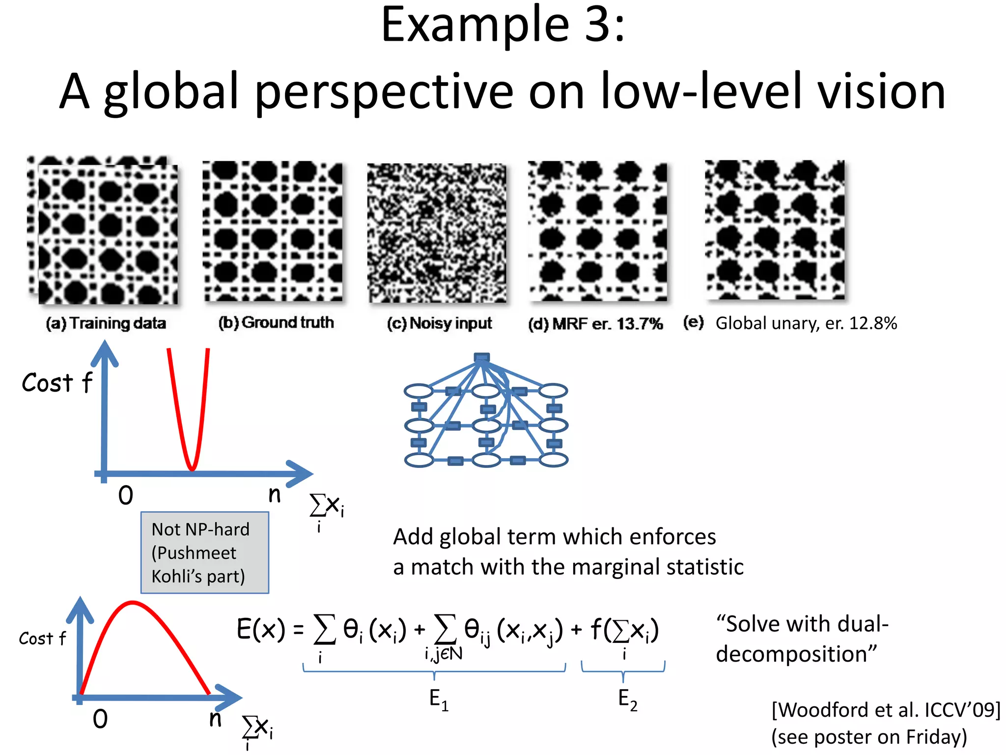
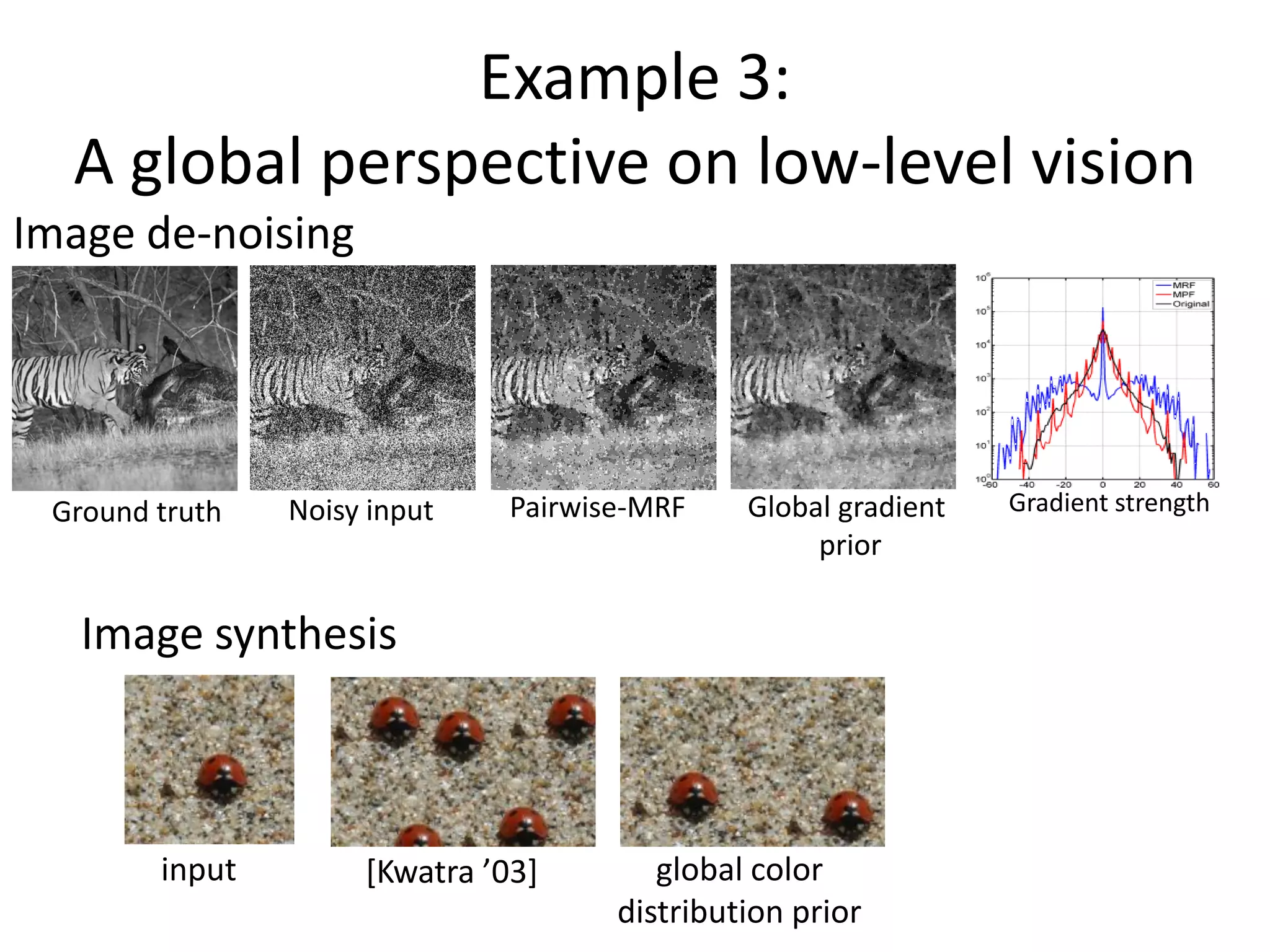
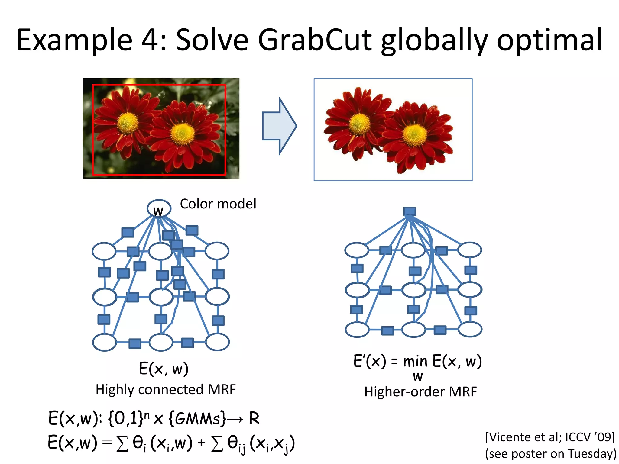
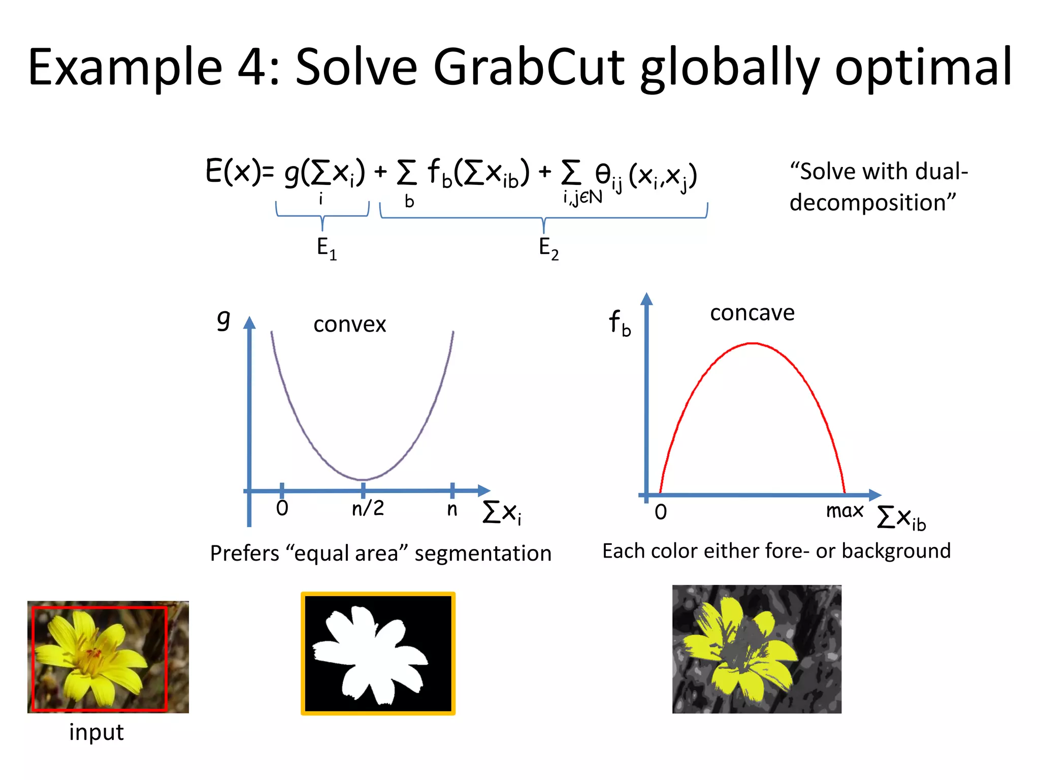
Dual Decomposition • Well known in optimization community [Bertsekas ’95, ‘99+ • Other names: “Master-Slave” [Komodiakis et al. ‘07, ’09+ • Examples of Dual-Decomposition approaches: – Solve LP of TRW [Komodiakis et al. ICCV ‘07+ – Image segmentation with connectivity prior [Vicente et al CVPR ‘08+ – Feature Matching [Toressani et al ECCV ‘08+ – Optimizing Higher-Order Clique MRFs [Komodiakis et al CVPR ‘09+ – Marginal Probability Field *Woodford et al ICCV ‘09+ – Jointly optimizing appearance and Segmentation [Vicente et al ICCV 09]

Dual Decomposition Hard to optimize Possible to optimize Possible to optimize min E(x) = min [ E1(x) + θTx + E2(x) – θTx ] x x ≥ min [E1(x1) + θTx1] + min [E2(x2) - θTx2] = L(θ) x1 x2 “Lower bound” • θ is called the dual vector (same size as x) • Goal: max L(θ) ≤ min E(x) θ x • Properties: • L(θ) is concave (optimal bound can be found) • If x1=x2 then problem solved (not guaranteed)

Why is the lower bound a concave function? L(θ) = min [E1(x1) + θTx1] + min [E2(x2) - θTx2] L(θ) : Rn -> R x1 x2 L1(θ) L2(θ) θTx’1 L1(θ) θTx’’1 θTx’’’1 θ L(θ) concave since a sum of concave functions

How to maximize the lower bound? If L(θ) were to be differentiable use gradient ascent L(θ) not diff. … so subgradient approach [Shor ‘85+

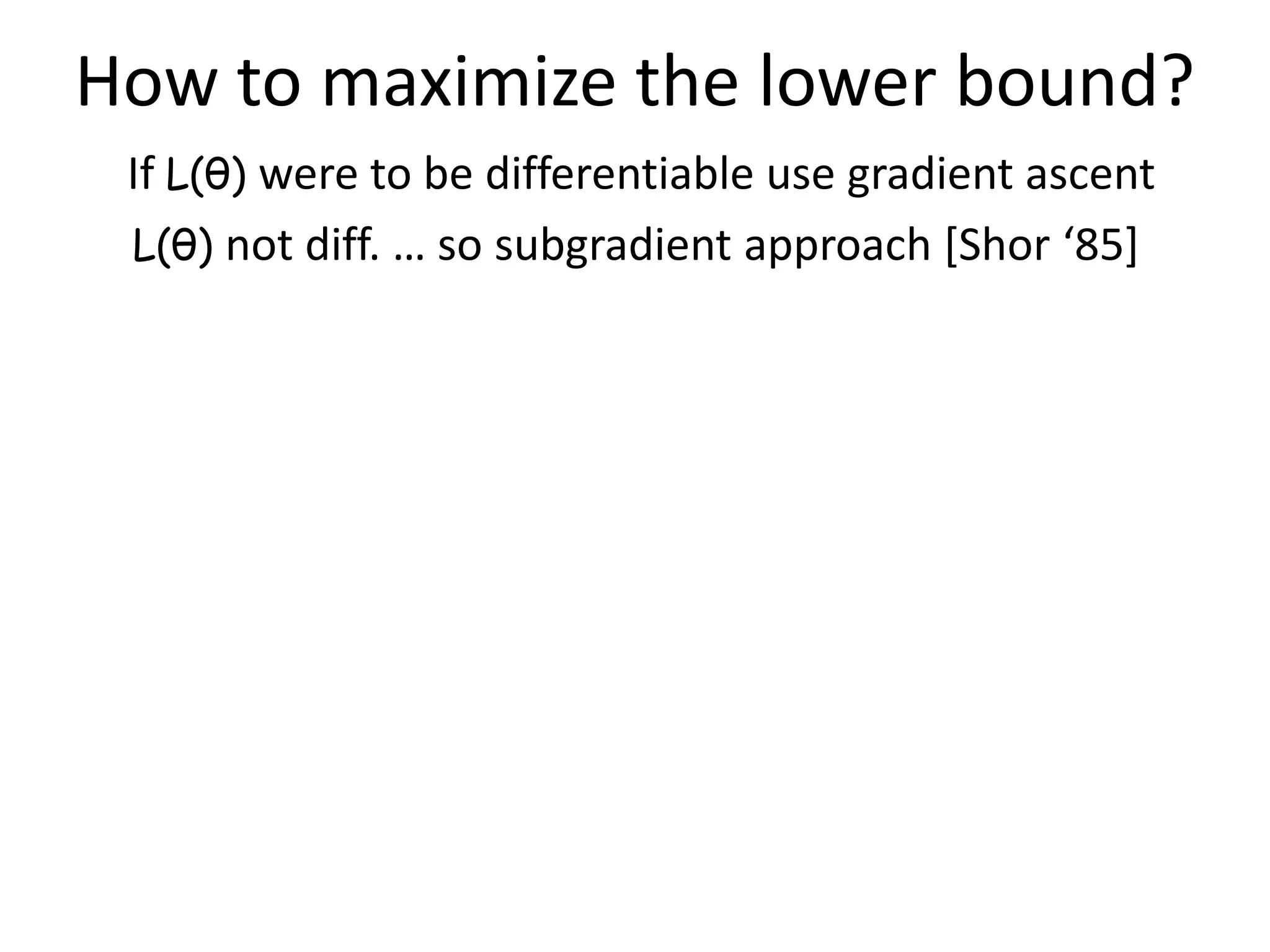
How to maximize the lower bound? If L(θ) were to be differentiable use gradient ascent L(θ) not diff. so subgradient approach [Shor ‘85+ L(θ) = min [E1(x1) + θTx1] + min [E2(x2) - θTx2] L(θ) : Rn -> R x1 x2 L1(θ) L2(θ) θTx’1 L1(θ) θTx’’1 Subgradient g θTx’’’1 Θ’ Θ’’ Θ Θ’’ = Θ’ + λ g = Θ’ + λ x’1 Θ’’ = Θ’ + λ (x1-x2)

Dual Decomposition L(θ) = min [E1(x1) + θTx1] + min [E2(x2) - θTx2] x1 x2 Subgradient Optimization: “Master” Θ = Θ + λ(x*-x2) 1 * x1* x2 * Θ Θ subgradient Subproblem 1 Subproblem 2 x* = min [E1(x1) + θTx1] 1 x2 = min [E2(x2) + θTx2] * “Slaves” x1 x2 • Guaranteed to converge to optimal bound L(θ) • Choose step-width λ correctly ([Bertsekas ’95]) • Pick solution x as the best of x1 or x2 • E and L can in- and decrease during optimization • Each step: θ gets close to optimal θ* Example optimization

Why can the lower bound go down? Lower envelop of planes in 3D: L(θ) L(θ’) L(θ’) ≤ L(θ)

Analyse the model push x1p towards 0 1 push x2p towards 1 0 L(θ) = min [E1(x1) + θTx1] + min [E2(x2) - θTx2] Update step: Θ’’ = Θ’ + λ (x*-x*) 1 2 Look at pixel p: Case1: x* = x2p 1p * then Θ’’ = Θ’ Case2: x* = 1 x2p = 0 1p * then Θ’’ = Θ’+ λ Case3: x* = 0 x* = 1 1p 2p then Θ’’ = Θ’- λ

Example 1: Segmentation and Connectivity Foreground object must be connected: E(x) = ∑ θi (xi) + ∑ θij (xi,xj) + h(x) h(x)= { ∞ if x not 4-connected 0 otherwise Zoom in User input Standard MRF Standard MRF +h *Vicente et al ’08+

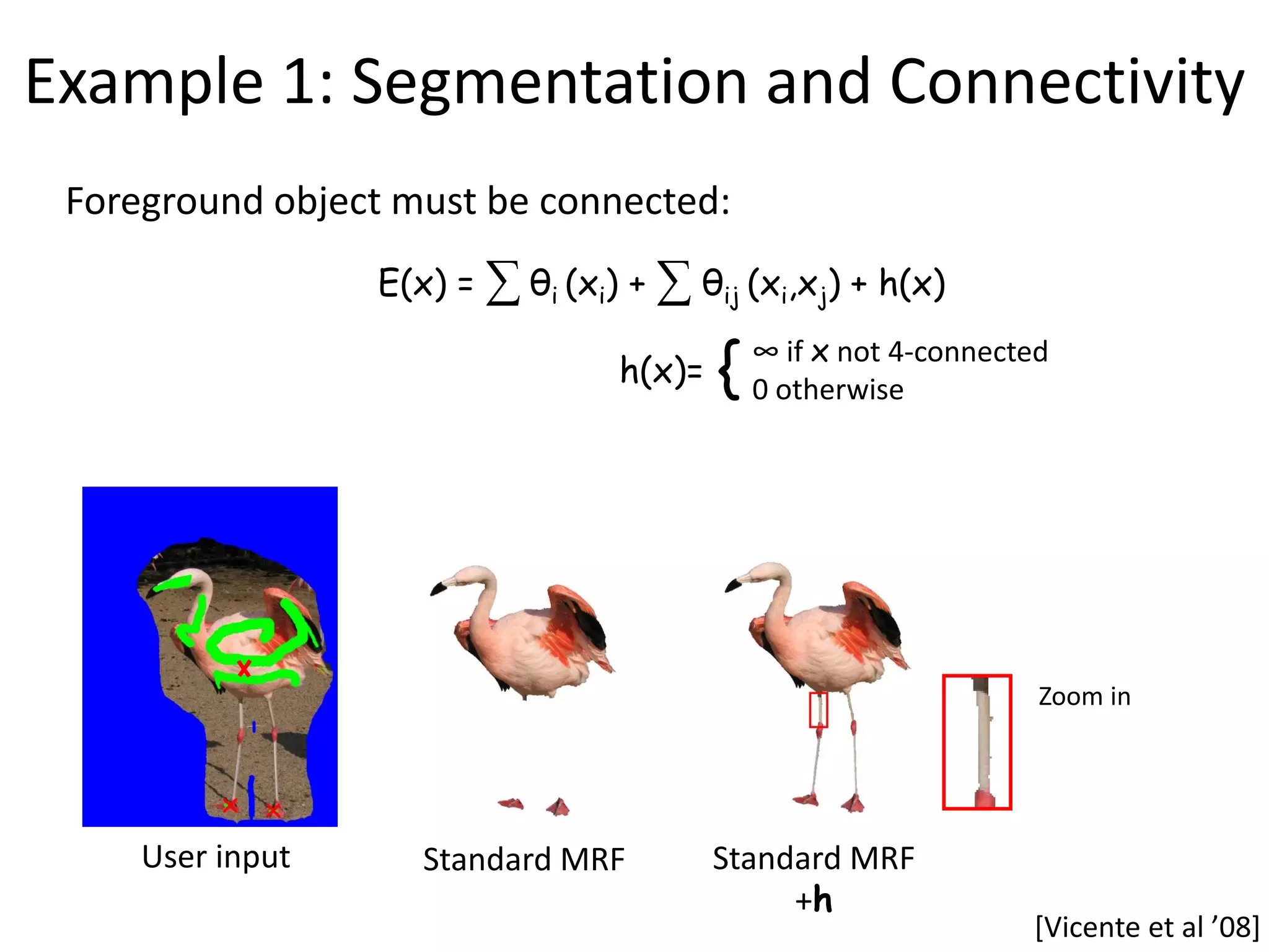
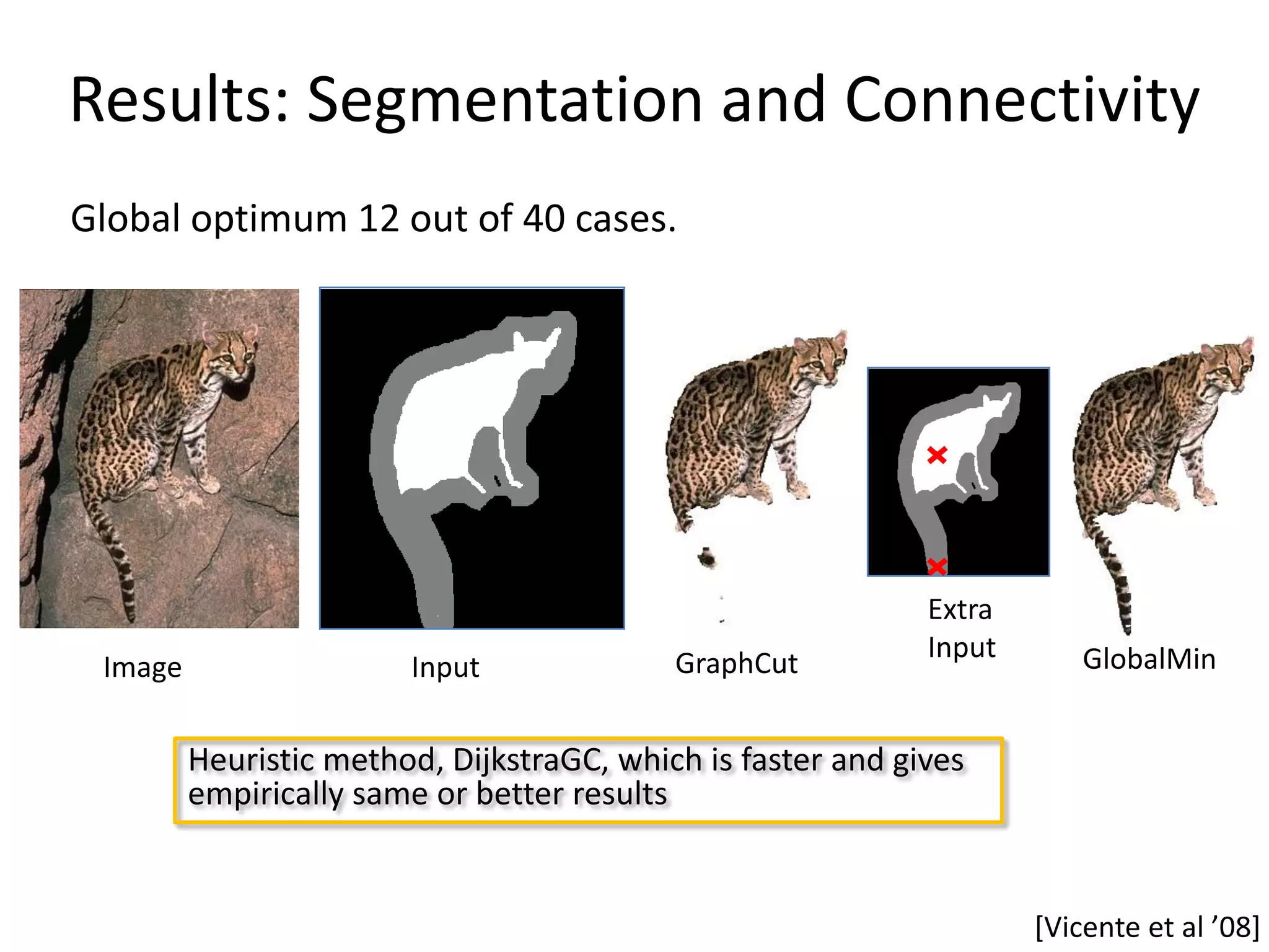
Example 1: Segmentation and Connectivity E1(x) E(x) = ∑ θi (xi) + ∑ θij (xi,xj) + h(x) h(x)= { ∞ if x not 4-connected 0 otherwise Derive Lower bound: min E(x) = min [ E1(x) + θTx + h(x) – θTx ] x x ≥ min [E1(x1) + θTx1] + min [h(x2) + θTx2] = L(θ) x1 x2 Subproblem 1: Subproblem 2: Unary terms + Unary terms + pairwise terms Connectivity constraint Global minimum: Global minimum: GraphCut Dijkstra But: Lower bound was for no example tight.

Example 1: Segmentation and Connectivity E1(x) E(x) = ∑ θi (xi) + ∑ θij (xi,xj) + h(x) h(x)= { ∞ if x not 4-connected 0 otherwise Derive Lower bound: x’ indicator vector of all pairwise terms min E(x) = min [ E1(x) + θTx + θ’Tx’ + h(x) – θTx + h(x) - θ’Tx’] x,x’ x,x’ ≥ min [E1(x1) + θTx1 + θ’Tx’1] + min [h(x2) + θTx2] + x1,x’1 x2 min [h(x3) + θ’Tx’3] =L(θ) x3,x’3 Subproblem 1: Subproblem 2: Subproblem 3: Unary terms + Unary terms + Pairwise terms + pairwise terms Connectivity constraint Connectivity constraint Global minimum: Global minimum: Lower Bound: Based on GraphCut Dijkstra minimal paths on a dual graph

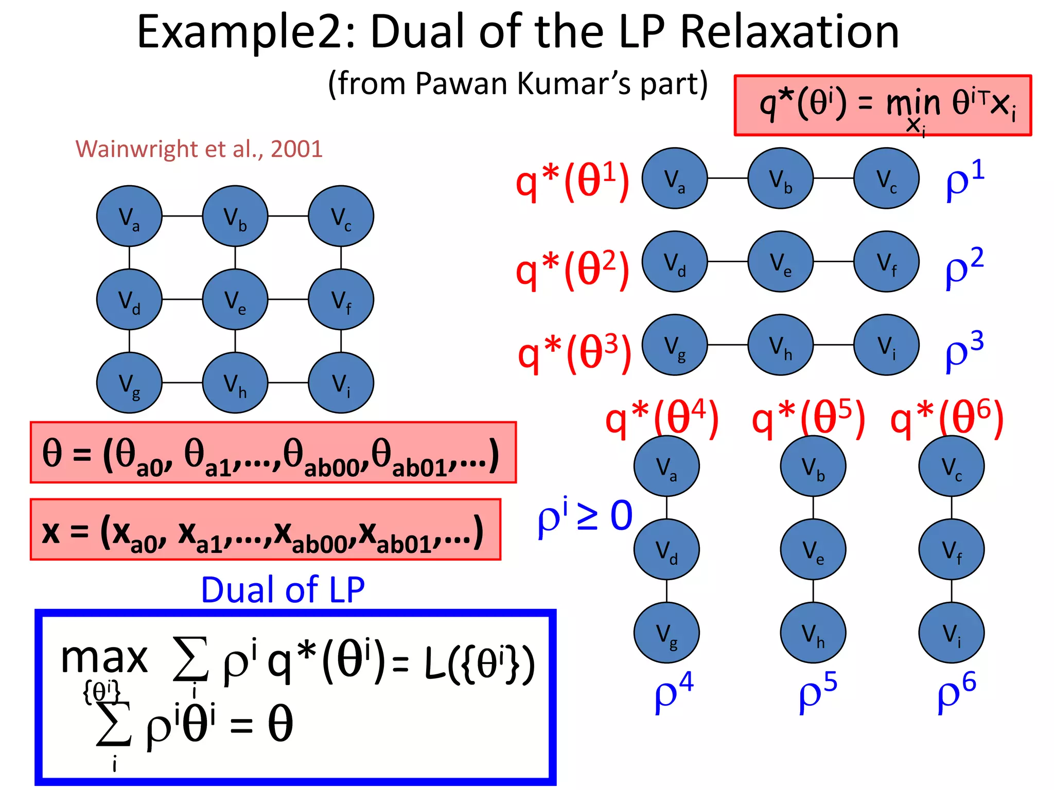
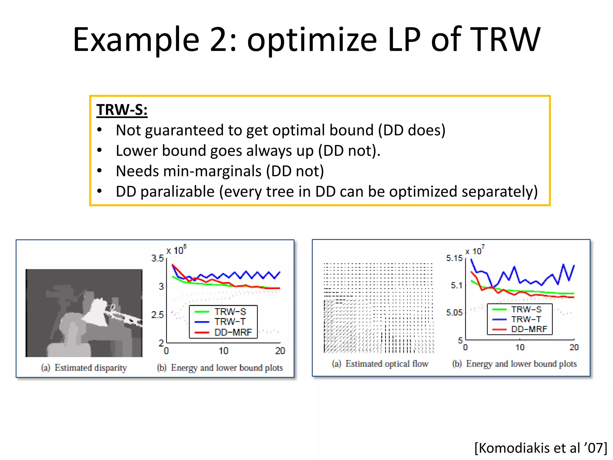
Results: Segmentation and Connectivity Global optimum 12 out of 40 cases. Extra Input GlobalMin Image Input GraphCut Heuristic method, DijkstraGC, which is faster and gives empirically same or better results *Vicente et al ’08+

Example2: Dual of the LP Relaxation (from Pawan Kumar’s part) q*( i) = min iTx i xi Wainwright et al., 2001 1 q*( 1) Va Vb Vc Va Vb Vc 2 q*( 2) Vd Ve Vf Vd Ve Vf 3 q*( 3) V V g V h i Vg Vh Vi q*( 4) q*( 5) q*( 6) =( a0, a1,…, ab00, ab01,…) Va Vb Vc i≥ 0 x = (xa0, xa1,…,xab00,xab01,…) Vd Ve Vf Dual of LP Vg Vh Vi max i q*( i) = L({ i}) { i} i 4 5 6 i i = i

Example2: Dual of the LP Relaxation “Original “i different “Lower bound” problem” trees” min Tx = min iTx x ∑ ≥ ∑ min x iTx i = L({ i}) x i i i q*( i) Subject to i = i Use subgradient … why? θTx’1 q*( i) concave wrt i ; q*( i) = min iTx i θTx’’1 xi θTx’’’1 Projected subgradient method: θ Θi = [Θi + λx *] i Ω Ω= {Θi| ∑ Θi = Θ } i Guaranteed to get the optimal lower bound !

Example 2: optimize LP of TRW TRW-S: • Not guaranteed to get optimal bound (DD does) • Lower bound goes always up (DD not). • Needs min-marginals (DD not) • DD paralizable (every tree in DD can be optimized separately) [Komodiakis et al ’07+

Example 3: A global perspective on low-level vision Global unary, er. 12.8% Cost f 0 n ∑xi Not NP-hard i Add global term which enforces (Pushmeet Kohli’s part) a match with the marginal statistic Cost f E(x) = ∑ θi (xi) + ∑ θij (xi,xj) + f(∑xi) “Solve with dual- i i,jЄN i decomposition” E1 E2 0 n ∑xi *Woodford et al. ICCV’09+ i (see poster on Friday)

Example 3: A global perspective on low-level vision Image de-noising Ground truth Noisy input Pairwise-MRF Global gradient Gradient strength prior Image synthesis input [Kwatra ’03+ global color distribution prior

Example 4: Solve GrabCut globally optimal w Color model E(x, w) E’(x) = min E(x, w) w Highly connected MRF Higher-order MRF E(x,w): {0,1}n x {GMMs}→ R E(x,w) = ∑ θi (xi,w) + ∑ θij (xi,xj) *Vicente et al; ICCV ’09+ (see poster on Tuesday)

Example 4: Solve GrabCut globally optimal E(x)= g(∑xi) + ∑ fb(∑xib) + ∑ θij (xi,xj) “Solve with dual- i b i,jЄN decomposition” E1 E2 g convex fb concave 0 n/2 n ∑xi 0 max ∑xib Prefers “equal area” segmentation Each color either fore- or background input

Example 3: Solve GrabCut globally optimal Globally optimal in 60% of cases, such as… *Vicente et al; ICCV ’09+ (see poster on Tuesday)

Summary • Dual Decomposition is a powerful technique for challenging MRFs • Not guaranteed to give globally optimal energy • … but for several vision problems we get tight bounds

Texture Restoration (table 1) 256x85 nodes; 15connec; 36% non-sub; 6.6 unary strength Training Image Test Image GC, E=999 QPBO, QPBOP, (0.05sec) 16.5% unlab. 0% unlab. (14sec) (1.4sec) Global Minimum. Sim. ann., ICM, BP, BP+I, C+BP+I (visually similar)

New-View Synthesis [Fitzgibbon et al ‘03] 385x385 nodes; 8con; 8% non-sub; 0.1 unary strength Ground Truth Graph Cut E=2 (0.3sec) Sim. Ann. E=980 (50sec) ICM E=999 (0.2sec) (visually similar) QPBO 3.9% unlabelled QPBOP - Global Min. (1.4sec), BP E=18 (0.6sec) (black) (0.7sec) P+BP+I, BP+I

Image Segmentation – region & boundary brush 321x221 nodes; 4con; 0.006% non-sub; 0 unary strength Input Image User Input Sim. Ann. E=983 (50sec) ICM E=999 (0.07sec) GraphCut E=873 (0.11sec) BP E=28 (0.2sec) QPBO 26.7% unlabeled QPBOP Global Min (3.8sec) (0.08sec)

Non-truncated cost function [HBF; Szeliski ‘06+ Fast linear system solver in continuous domain (then discretised) cost |di-dj| original input HBF

ICCV2009: MAP Inference in Discrete Models: Part 5

More Related Content

Viewers also liked

Similar to ICCV2009: MAP Inference in Discrete Models: Part 5

More from zukun

Recently uploaded

ICCV2009: MAP Inference in Discrete Models: Part 5