Downloaded 445 times

![Initialization: Sort the n objects from large to small based on their ratios vi / wi . We assume the arrays w[1..n] and v[1..n] store the respective weights and values after sorting. initialize array x[1..n] to zeros. weight = 0; i = 1; THE OPTIMAL KNAPSACK ALGORITHM](https://image.slidesharecdn.com/greedy-170403085712/75/Greedy-Algorithm-Knapsack-Problem-11-2048.jpg)
![while (i n and weight < W) do if weight + w[i] W then x[i] = 1 else x[i] = (W – weight) / w[i] weight = weight + x[i] * w[i] i++ THE OPTIMAL KNAPSACK ALGORITHM](https://image.slidesharecdn.com/greedy-170403085712/75/Greedy-Algorithm-Knapsack-Problem-12-2048.jpg)
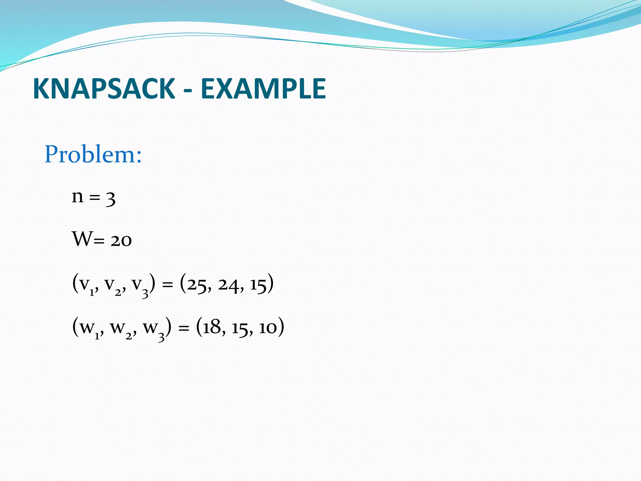
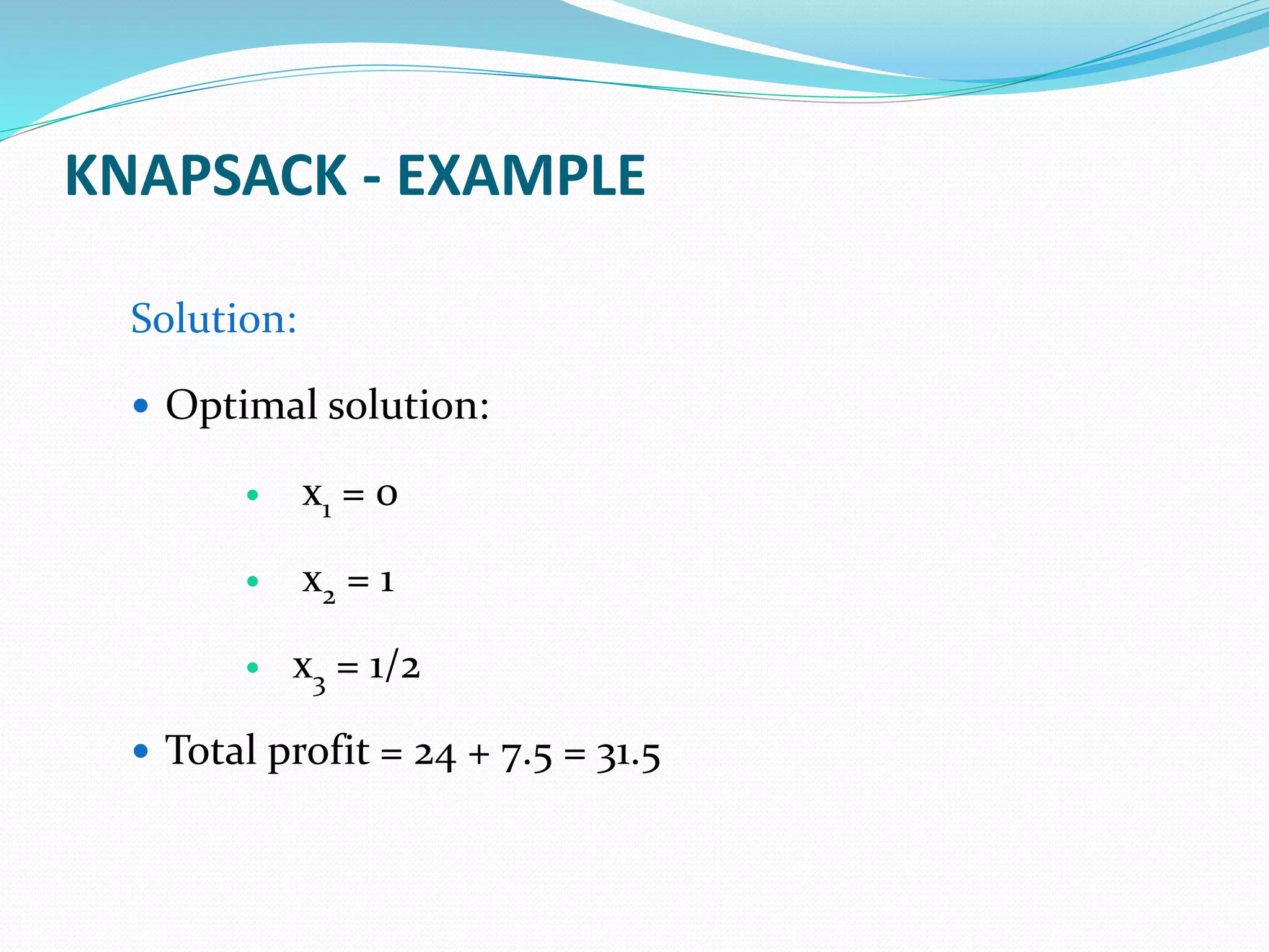


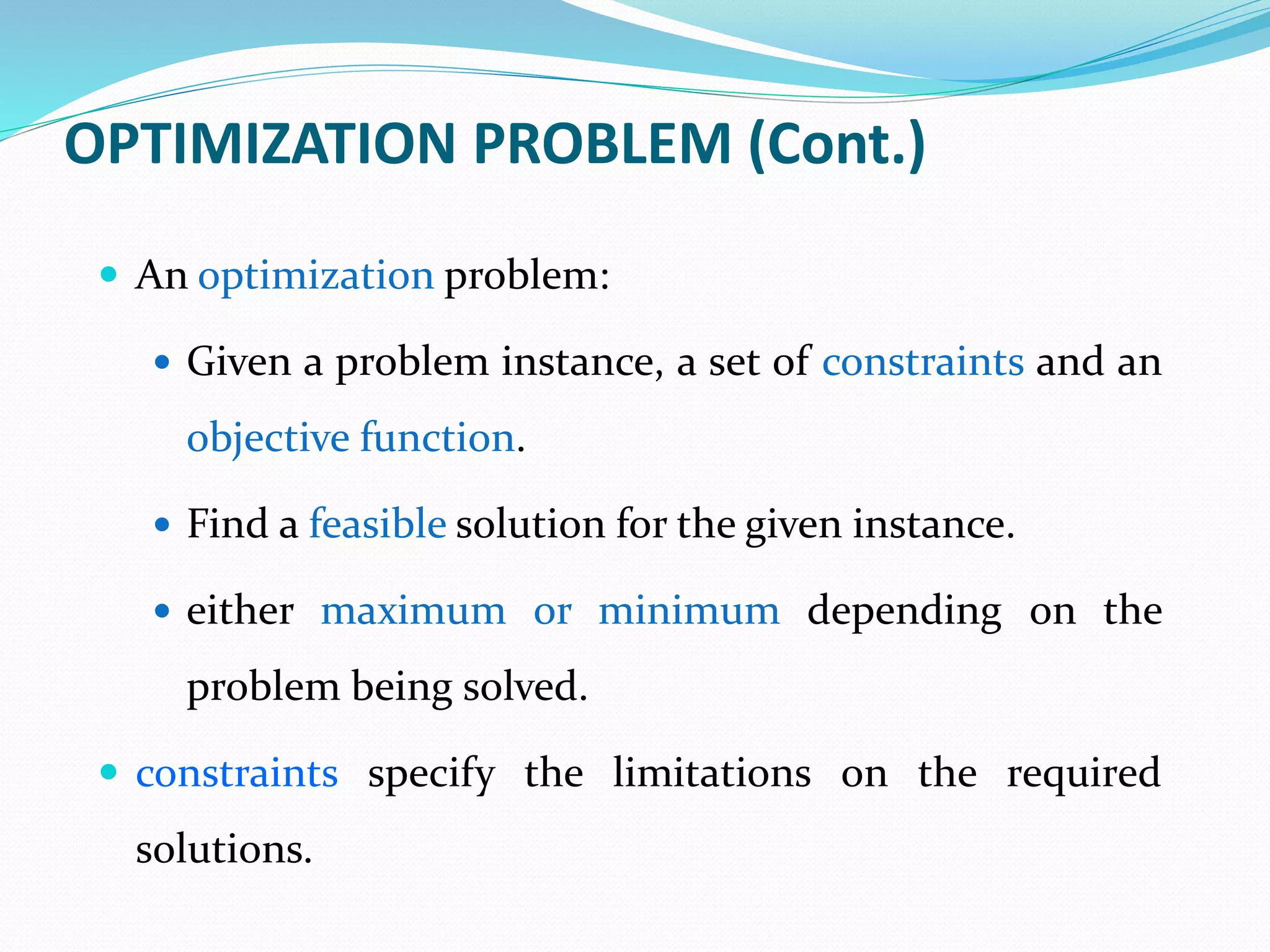
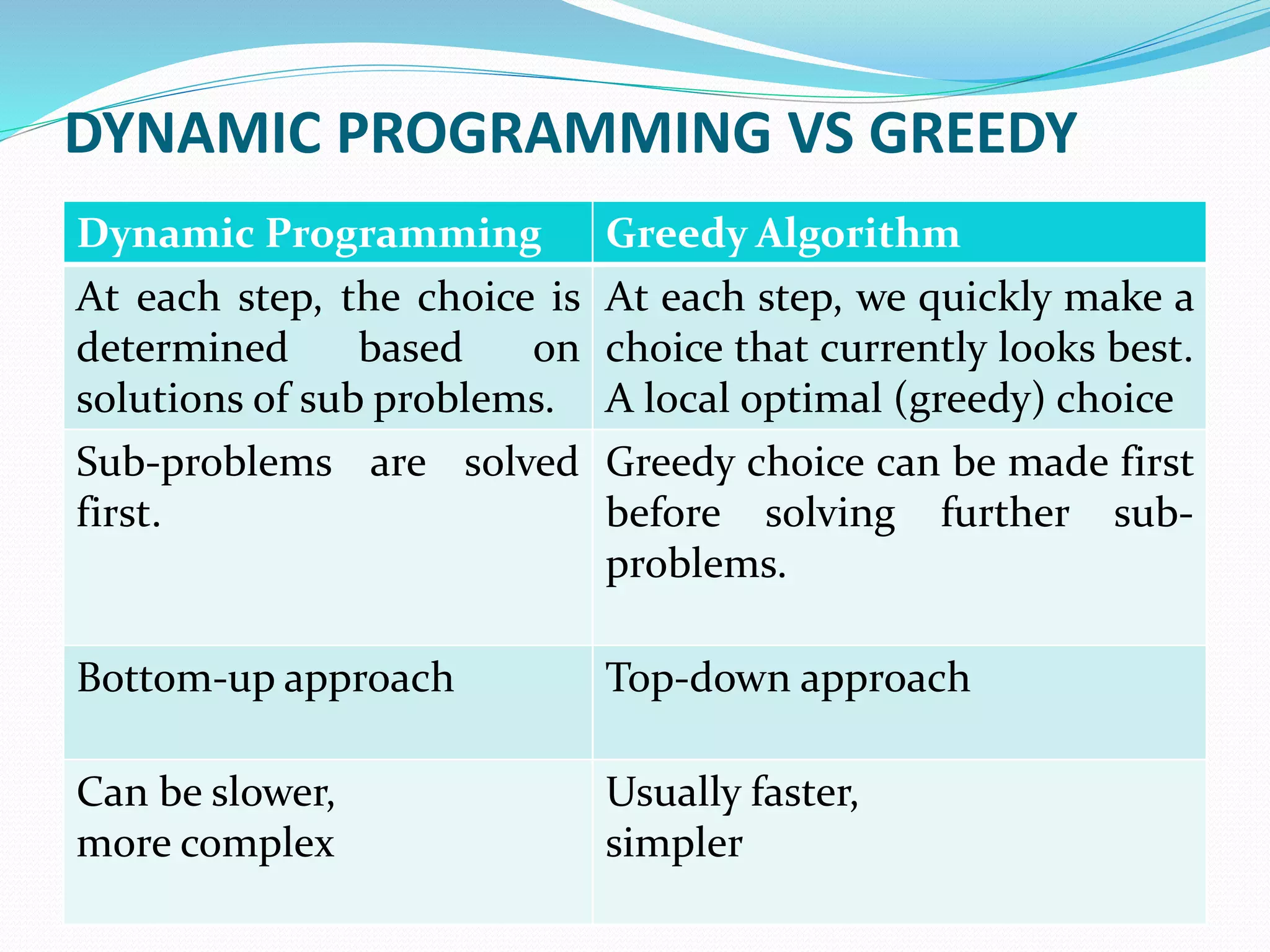
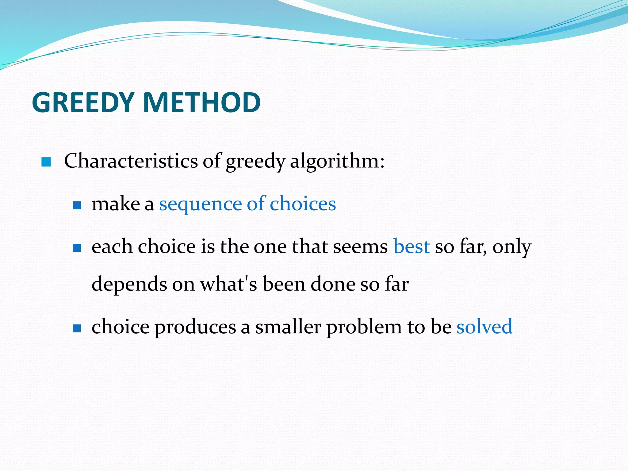
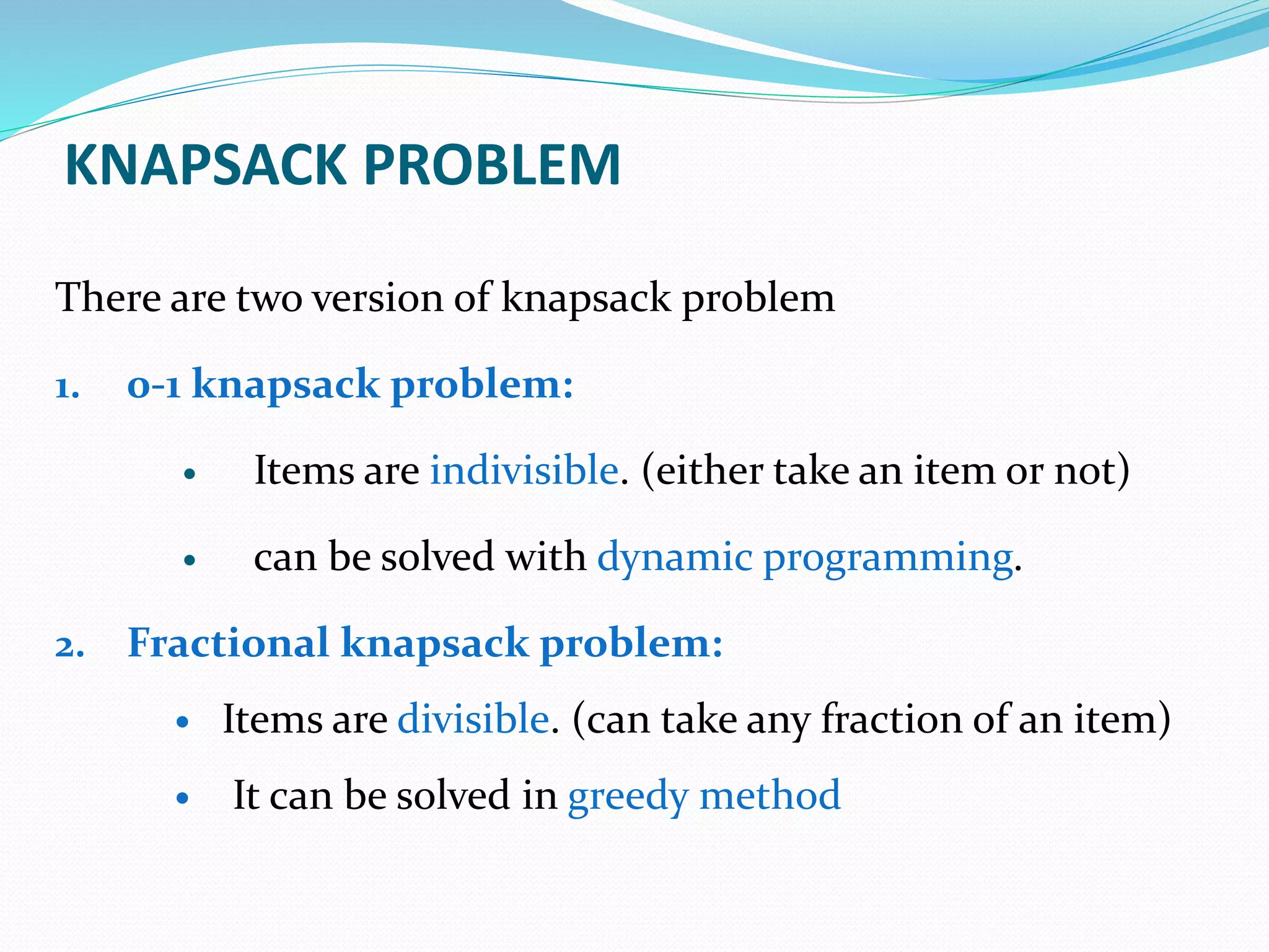
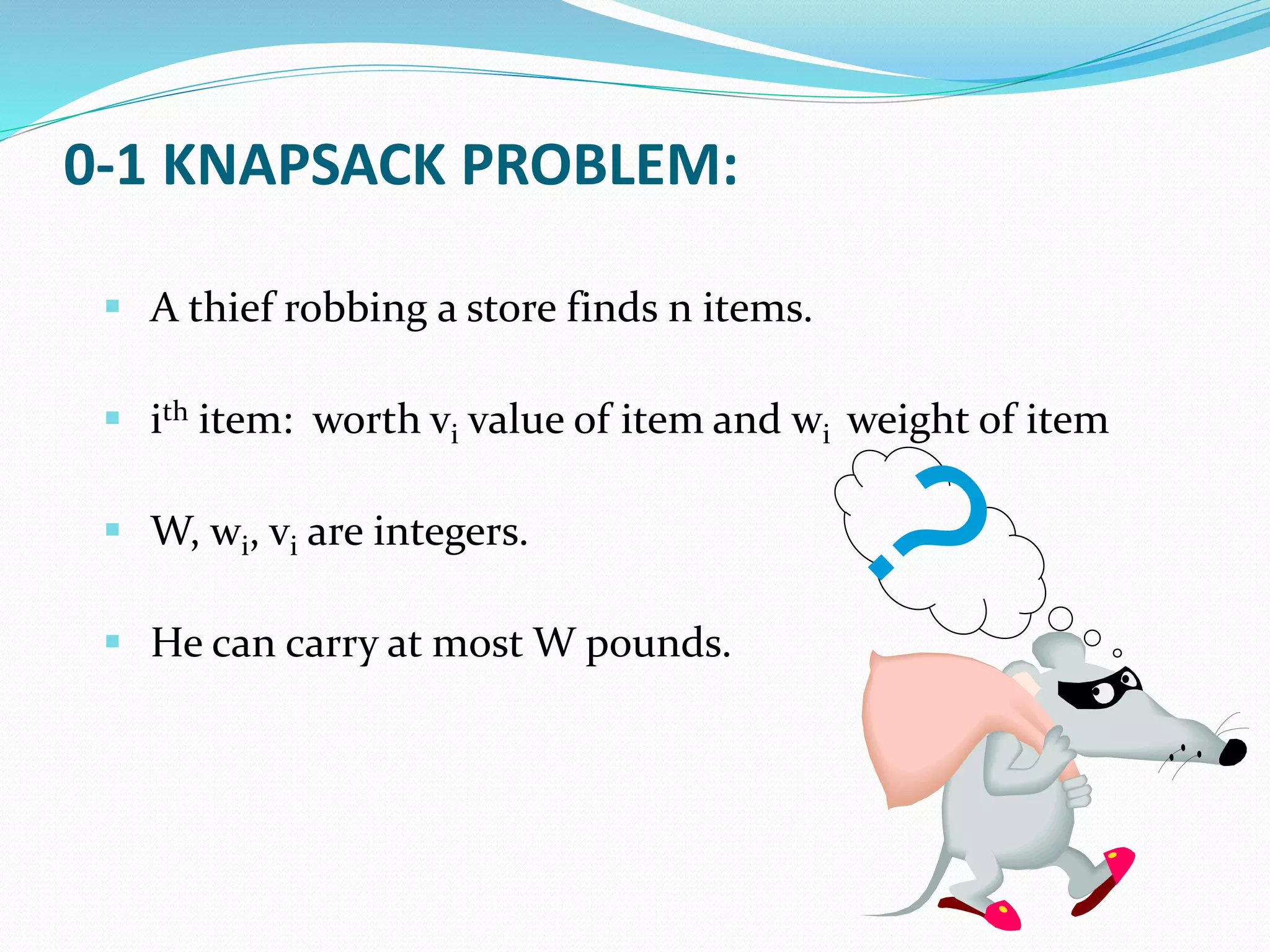
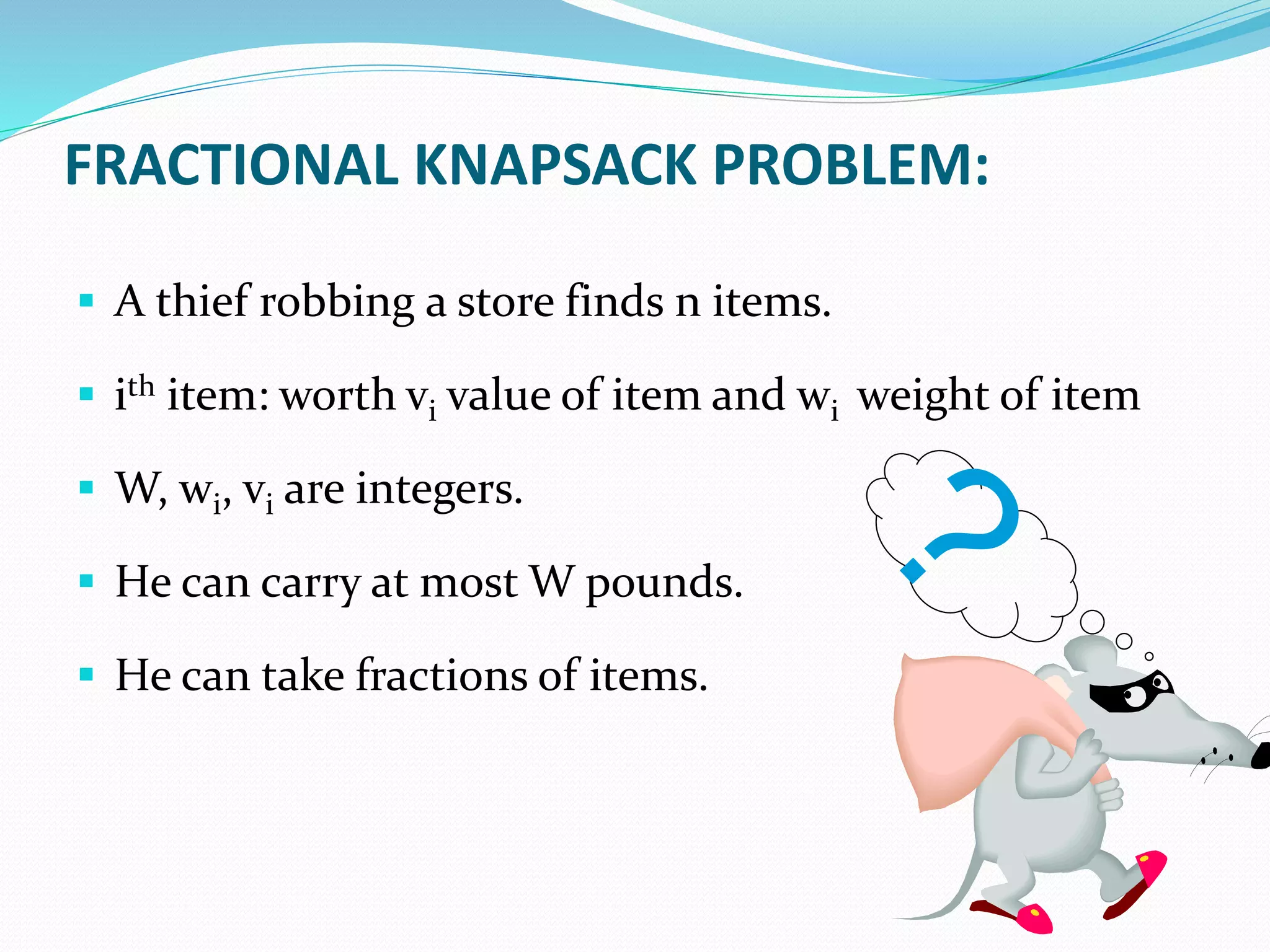
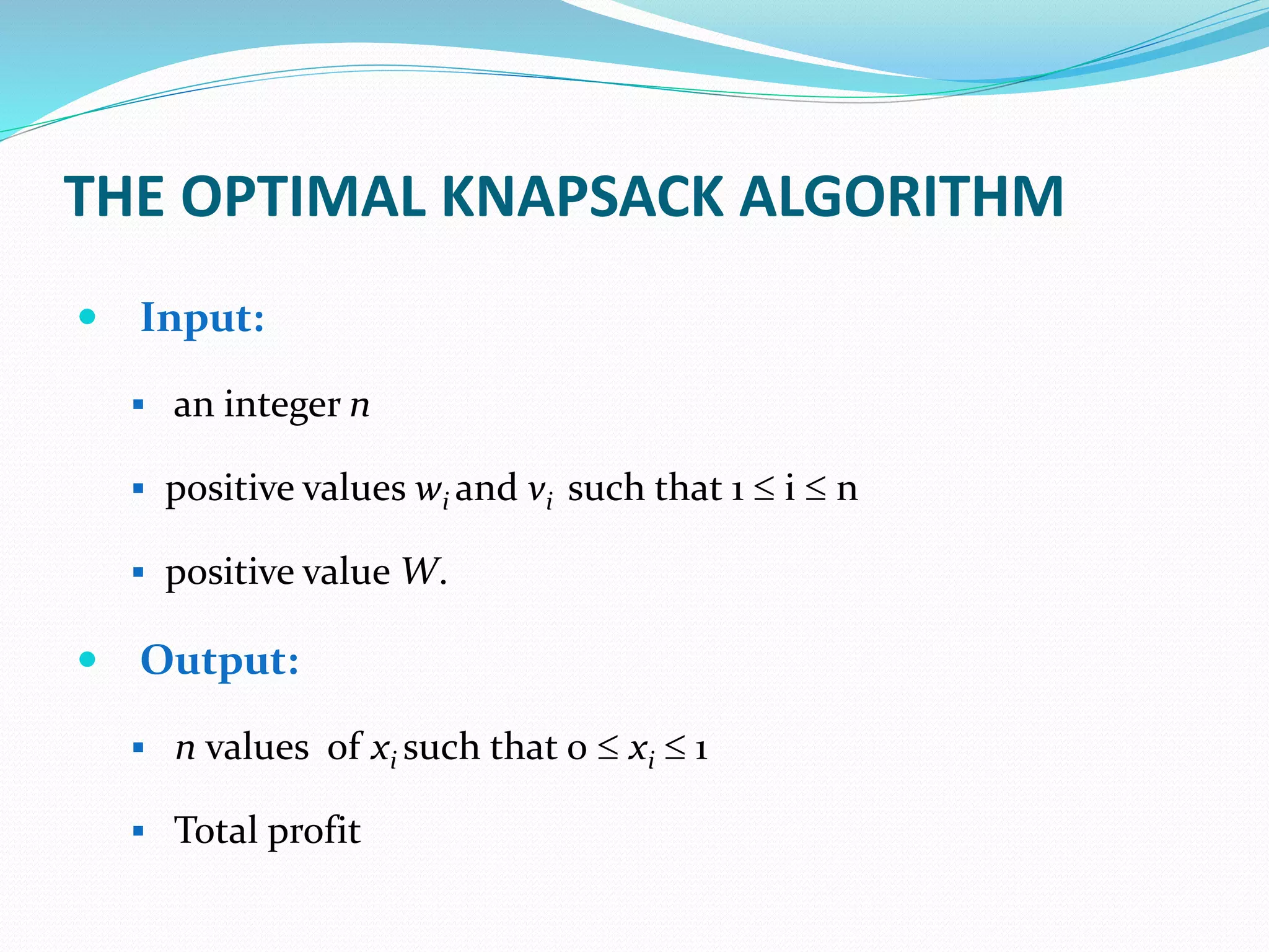
The document discusses the knapsack problem and greedy algorithms. It defines the knapsack problem as an optimization problem where given constraints and an objective function, the goal is to find the feasible solution that maximizes or minimizes the objective. It describes the knapsack problem has having two versions: 0-1 where items are indivisible, and fractional where items can be divided. The fractional knapsack problem can be solved using a greedy approach by sorting items by value to weight ratio and filling the knapsack accordingly until full.