Download to read offline
![International Research Journal of Engineering and Technology (IRJET) e-ISSN: 2395-0056 Volume: 09 Issue: 04 | Apr 2022 www.irjet.net p-ISSN: 2395-0072 © 2022, IRJET | Impact Factor value: 7.529 | ISO 9001:2008 Certified Journal | Page 1363 Finding the Relational Description of Different Objects and Their Importance in a Scene Sabyasachi Moitra1, Sambhunath Biswas1,2 1Dept. of Comp. Sc. & Engg., Techno India University, West Bengal, India 2Ex-Indian Statistical Institute, Kolkata, India ---------------------------------------------------------------------***--------------------------------------------------------------------- Abstract - A scene is composed of many objects. It is needless to say, that these objects have some relational description between them. The relative positions of different objects in a scene define the relational description between its near and far objects with respect to an observer. Such a relational description is not only significant from different perspectives but also is important in many useful applications. In this paper, we propose two different methods to find the relative positions of objects in a scene and based on this information, a hierarchical description or a tree structure is generated. This structure has an immense role in scene estimation and processing of various applications. One of the methods considers simply the Euclidean distance between the image baseline and different objects in the scene. The other method computes the distance considering the depth map of the objects. To study the superiority of the methods, we have made a comparison between them. It is seen that the first method is simpler and faster compared to the second one. We also determine the weights of different objects based on their hierarchical description, which may find an immense role in determining the importance of various objects present in the scene. Key Words: Object detection, Object position, Object hierarchy, Object weights. 1. INTRODUCTION Object detection is a well-known problem in computer vision community to identify and locate objects in a static or dynamic scene, such as a video. The technique draws bounding boxes around detected objects, allowing us to determine the object location and the object class in a given scene. The problem has widespread applications; some of them include self-driving cars, video surveillance, crowd counting, etc. Object detection methods can be divided in two categories that use (i) classical computer vision techniques and the (ii) modern or deep learning- based techniques. Classical computer vision techniques extract features from an image to identify an object. This finds applications favouring methods described in Viola-Jones [1], HOG [2]. The features for objects are fed into a pre-trained classifier, such as SVM, for prediction of the objects' classes. A sliding window at different positions in images can be used to extract features. These features may or may not correspond to an object at a particular position. In other words, the sliding window locates positions of different objects. On the other hand, in deep learning- based techniques, a deep convolutional neural network [3][4] is used to extract features from an image to classify and localize an object, such as in R-CNN [5], Faster R-CNN [6], and YOLO [7]. For classification and localization of objects in images, these features are fed into a sequence of fully-connected layers or convolutional layers. A convolutional neural network is made up of a series of convolutional and max-pool layers. To analyze a given scene, the relationships between the detected objects in the scene must be known. This means the relative position of each object with respect to an observer as well as other detected objects are made known (e.g., the current position of each sprinter in a sprint). This paper, presents two methods for determining such relative position of detected objects. This relative positional structure provides a hierarchical description of objects. The hierarchy has a significant impact in different applications. This is ensured through different weights attached to different detected objects. The weights are computed based on their relative positions in the scene. 2. CAMERA-OBJECT DISTANCE To find the camera-object distance, we assume that a camera is placed on the z-axis and is horizontal. This is a usual practice. One can have some idea about the camera positioning as referred to in [8]. Objects can, initially be detected using a cutting-edge object detection method. We have used YOLO [7] in our algorithm. The distance between the camera and detected objects is, subsequently computed. This provides the relative position of detected objects in a scene with respect to an observer. We have proposed two different methods to compute the camera- object distance. The first one is simple in nature, while the second one uses the concept based on depth map described in [9]. Method-1: Method-1 uses an RGB image (scene) as input as shown in Figure 1 and detects objects as indicated in it. It computes](https://image.slidesharecdn.com/irjet-v9i4237-220923120723-1e23ce9d/75/Finding-the-Relational-Description-of-Different-Objects-and-Their-Importance-in-a-Scene-1-2048.jpg)
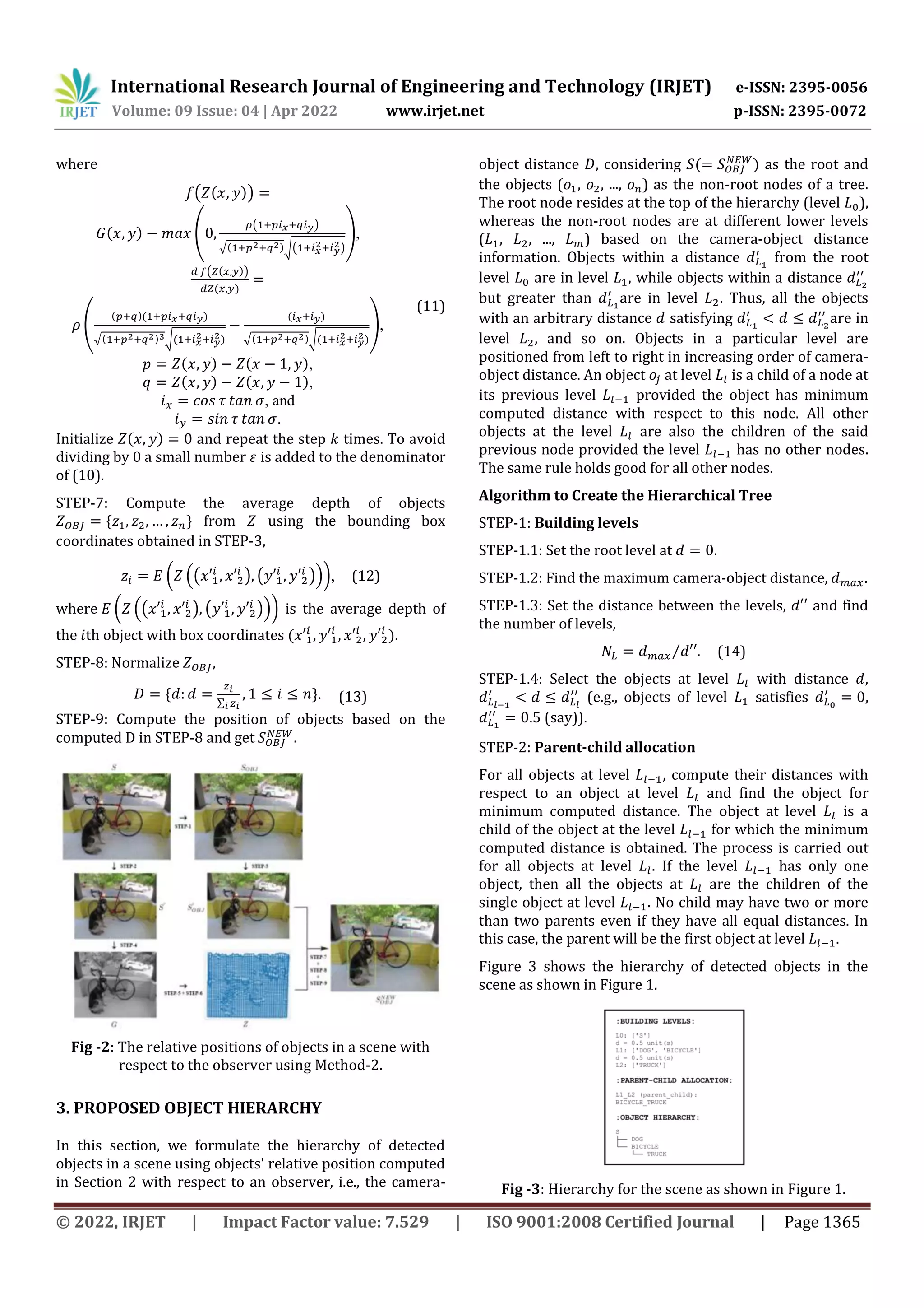
![International Research Journal of Engineering and Technology (IRJET) e-ISSN: 2395-0056 Volume: 09 Issue: 04 | Apr 2022 www.irjet.net p-ISSN: 2395-0072 © 2022, IRJET | Impact Factor value: 7.529 | ISO 9001:2008 Certified Journal | Page 1364 the camera-object distance using the orthogonal distance between the image baseline and the detected objects. The related algorithm is stated below. Algorithm STEP-1: Detect objects in a scene, using the YOLO model, YOLO( ) .[ ] /, (1) where [ ] is a vector in which ( ) are the th bounding box coordinates, i.e., location (( ) and ( ) are the top-left and bottom-right corners respectively) and is the class of the th object detected. STEP-2: For each object in : STEP-2.1: Draw a perpendicular from the bottom-right corner of its bounding box ( ) to the baseline of . STEP-2.2: Calculate the length of ( ) by computing the Euclidean distance between ( ) and the point perpendicularly located on 's baseline ( ), ( ) √∑ ( ) , (2) where ( ) is the Euclidean distance between two points and with ( ) and ( ) ( → bottom-right corner of ). STEP-3: Normalize the perpendicular distances computed in STEP-2, * ∑ +. (3) STEP-4: Compute the position of objects based on the computed in STEP-3 and get . Fig -1: The relative positions of objects in a scene with respect to the observer using Method-1. Method-2 (Depth Map-Based): Depth map-based method has its framework in [10]. It also inputs the same RGB image (scene) and detects objects as shown in Figure 2, but it computes the camera-object distance by computing the average of the depth map image of the detected object. Algorithm STEP-1: Detect objects in using the YOLO model, YOLO( ) .[ ] /, (4) where [ ] is a vector in which ( ) are the th bounding box coordinates, i.e., location (( ) and ( ) are the top-left and bottom-right corners respectively) and is the class of the th object detected. STEP-2: Resize to , , (5) where . STEP-3: For each object in , map ( ) on using [11], ( ⁄ ), ( ⁄ ), (6) .[ ] /, where * +. STEP-4: Convert to grayscale ( ) using the weighted/luminosity method [12], ( ) ( ) ( ), (7) where , , and are the red, green, and blue values of each pixel in , respectively. STEP-5: Compute the albedo (surface reflectivity of an object) ( ) and illumination direction ( ) [13] from , √ (8) , -, where ( ( )), (9) ( ( )), , and √ ( ( ( )) → average of the image brightness (pixel intensity), ( ( )) → average of the image brightness square, → tilt, → slant, → image's spatial gradient in direction, → image's spatial gradient in direction). STEP-6: Construct the depth map from using [10], ( ) ( ) ( ( )) ( ( )) ( ) , (10)](https://image.slidesharecdn.com/irjet-v9i4237-220923120723-1e23ce9d/75/Finding-the-Relational-Description-of-Different-Objects-and-Their-Importance-in-a-Scene-2-2048.jpg)
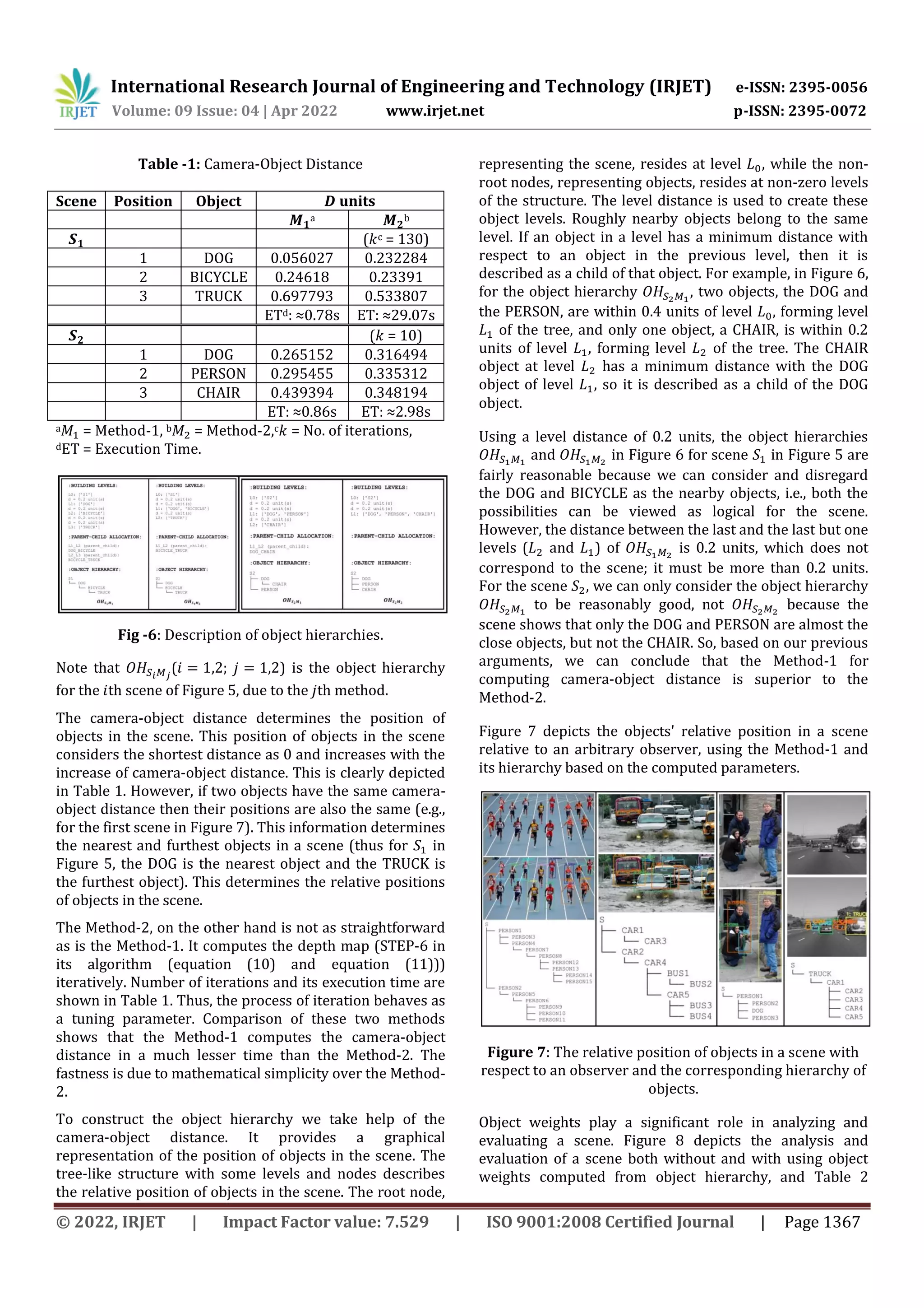
![International Research Journal of Engineering and Technology (IRJET) e-ISSN: 2395-0056 Volume: 09 Issue: 04 | Apr 2022 www.irjet.net p-ISSN: 2395-0072 © 2022, IRJET | Impact Factor value: 7.529 | ISO 9001:2008 Certified Journal | Page 1368 shows the significance of object weights in a comparative analysis for evaluations. Fig -8: Evaluation of a scene both without (top) and with (bottom) object weights. Table -2: Comparative Analysis Problem Chances of first, second and third place holders in a sprint as shown in Figure 8. Solution Without Using Object Weights Using Object Weights Interpretation Interpretation Both PERSON1 and PERSON2 have a chance of winning the first place, PERSON3, PERSON4, PERSON5 the second, and PERSON7 and PERSON6 the third. PERSON1 has a higher chance of winning the first place than PERSON2. If PERSON1 wins the first place, PERSON2 has a better chance of finishing second than PERSON3, PERSON4, and PERSON5. If PERSON2 takes second place, both PERSON3 and PERSON4 have a higher and equal probability of taking third place than PERSON5, PERSON6, and PERSON7. Inference Inference Impossibility for inferencing/decision making for winners. Ability for inferencing/decision making for winners. 6. CONCLUSION In this paper, we find objects' successive positions in a scene, by measuring the distance between an object and an observer (the camera). We have proposed two different methods, in which the first method computes the camera- object distance using the Euclidean distance between the image baseline and the detected objects, and the second method computes the same using the depth map of object. We have also created a hierarchical description of objects in a scene based on this information. This hierarchy is helpful to find the objects relative position in the scene and may find an immense role in analysis as well as in data structure of scenes. The data structure might be helpful in faster processing of scenes. The comparison between the methods shows that Method-1 is superior to Method-2 that uses the depth map of object. We have also computed the object weights from its hierarchical description in the scene. This plays an important role in analysis and evaluation of a scene. Our main objective is to make the whole system more robust and informative, and we shall describe the concerned method in a forthcoming paper. ACKNOWLEDGEMENT The authors would like to acknowledge Techno India University, West Bengal for its support to this work. REFERENCES [1] Viola P, Jones M. Rapid object detection using a boosted cascade of simple features. In: Proceedings of the 2001 IEEE Computer Society Conference on Computer Vision and Pattern Recognition. CVPR 2001. vol. 1; 2001. p. I–I. [2] Dalal N, Triggs B. Histograms of oriented gradients for human detection. In: 2005 IEEE Computer Society Conference on Computer Vision and Pattern Recognition (CVPR’05). vol. 1; 2005. p. 886–893. [3] Krizhevsky A, Sutskever I, Hinton GE. ImageNet Classification with Deep Convolutional Neural Networks. In: Advances in Neural Information Processing Systems 25. Curran Associates, Inc.; 2012. p. 1097–1105. [4] Simonyan K, Zisserman A. Very Deep Convolutional Networks for Large-Scale Image Recognition. CoRR. 2015;abs/1409.1556. [5] Girshick R, Donahue J, Darrell T, Malik J. Rich Feature Hierarchies for Accurate Object Detection and Semantic Segmentation. In: The IEEE Conference on Computer Vision and Pattern Recognition (CVPR); 2014.](https://image.slidesharecdn.com/irjet-v9i4237-220923120723-1e23ce9d/75/Finding-the-Relational-Description-of-Different-Objects-and-Their-Importance-in-a-Scene-6-2048.jpg)
![International Research Journal of Engineering and Technology (IRJET) e-ISSN: 2395-0056 Volume: 09 Issue: 04 | Apr 2022 www.irjet.net p-ISSN: 2395-0072 © 2022, IRJET | Impact Factor value: 7.529 | ISO 9001:2008 Certified Journal | Page 1369 [6] Ren S, He K, Girshick R, Sun J. Faster R-CNN: Towards Real-Time Object Detection with Region Proposal Networks. In: Advances in Neural Information Processing Systems 28. Curran Associates, Inc.; 2015. p. 91–99. [7] Redmon J, Divvala S, Girshick R, Farhadi A. You Only Look Once: Unified, Real-Time Object Detection. In: The IEEE Conference on Computer Vision and Pattern Recognition (CVPR); 2016. [8] Singh A, Singh S, Tiwari DS. Comparison of face Recognition Algorithms on Dummy Faces. International Journal of Multimedia & Its Applications. 2012 09;4. [9] Zhang R, Tsai PS, Cryer JE, Shah M. Shape-from- shading: a survey. IEEE Transactions on Pattern Analysis and Machine Intelligence. 1999;21(8):690– 706. https://doi.org/10.1109/34.784284. [10] Ping-Sing T, Shah M. Shape from shading using linear approximation. Image and Vision Computing. 1994;12(8):487–498. https://doi.org/10.1016/0262- 8856(94)90002-7. [11] Cogneethi.: C 7.5 | ROI Projection | Subsampling ratio | SPPNet | Fast RCNN | CNN | Machine learning | EvODN. Available from: https://www.youtube.com/watch?v=wGa6ddEXg7w& list=PL1GQaVhO4f jLxOokW7CS5kY J1t1T17S. [12] Dynamsoft.: Image Processing 101 Chapter 1.3: Color Space Conversion. Available from: https://www.dynamsoft.com/blog/insights/image- processing/image-processing-101-color-space- conversion/. [13] Zheng Q, Chellappa R. Estimation of illuminant direction, albedo, and shape from shading. IEEE Transactions on Pattern Analysis and Machine Intelligence. 1991;13(7):680–702. https://doi.org/10.1109/34.85658. BIOGRAPHIES Sabyasachi Moitra received his B.Sc. degree in Computer Science from the University of Calcutta, Kolkata, India, in 2012, M.Sc. degree in Computer Technology from The University of Burdwan, Burdwan, India, in 2014, and the M.Tech. degree in Computer Science and Engineering from Maulana Abul Kalam Azad University of Technology, West Bengal, India, in 2017. He is currently pursuing a Ph.D. degree in Computer Science and Engineering at Techno India University, West Bengal, India. His areas of interest are web technology, machine learning, deep learning, computer vision, and image processing. Sambhunath Biswas is a Senior Professor of Computer Science and Engineering in Techno India University, West Bengal, India and was formerly associated with the Machine Intelligence Unit, Indian Statistical Institute, Kolkata, India. He did his Ph.D. in Radiophysics and Electronics from the University of Calcutta in 2001. He was a UNDP Fellow at MIT, USA in 1988-89, visited the Australian National University at Canberra in 1995 to join the school on wavelets theory and its applications. In 2001, he visited China as a representative of the Government of India, Italy and INRIA in France in June 2010. He has published several research articles and is the principal author of the book Bezier and Splines in Image Processing and Machine Vision, published by Springer, London, and edited the first proceedings of PReMI (Pattern Recognition and Machine Intelligence) in 2005.](https://image.slidesharecdn.com/irjet-v9i4237-220923120723-1e23ce9d/75/Finding-the-Relational-Description-of-Different-Objects-and-Their-Importance-in-a-Scene-7-2048.jpg)

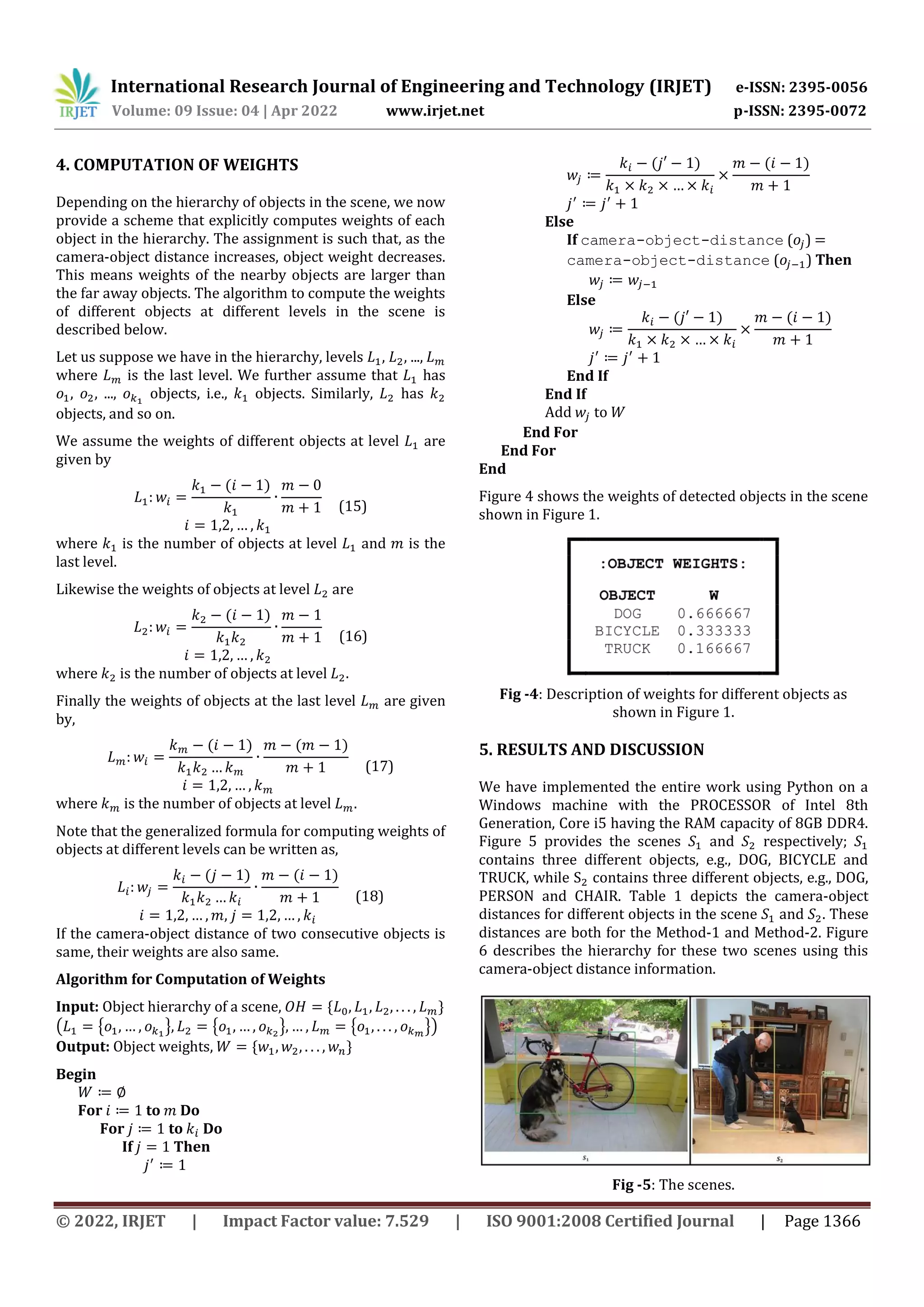
This document proposes two methods for determining the relative positions of objects detected in a scene. Method 1 simply calculates the Euclidean distance between objects and the image baseline. Method 2 computes distances using depth maps, which involves iterative depth map construction and is more computationally expensive. Both methods are used to generate a hierarchical description of objects in a scene as a tree structure. Object weights are also computed based on their position in the hierarchy, with nearer objects assigned higher weights. The first method is shown to be simpler and faster than the second method involving depth maps.