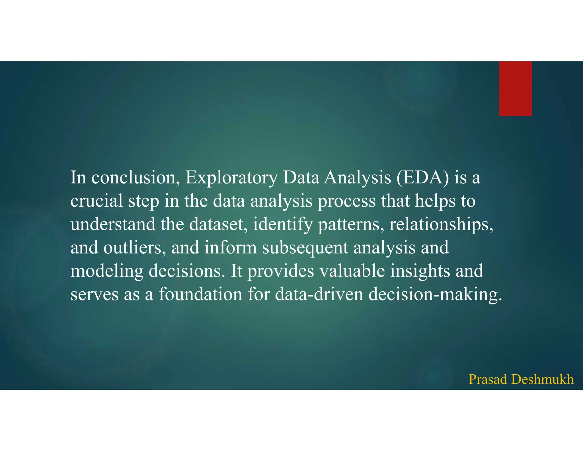
Exploratory Data Analysis in Machine Learning

Exploratory Data Analysis in Machine Learning

• 1.
  Exploratory Data Analysis PrasadDeshmukh
• 2.
   EDA isa crucial step in data analysis, involving data exploration, visualization, and summarization to uncover patterns and gain insights.  EDA helps to understand the structure and characteristics of the dataset, detect outliers, and identify relationships between variables through statistical analysis and visualizations. Exploratory Data Analysis Prasad Deshmukh
• 3.
  Data Collection  Obtainthe dataset you want to analyze.  This may involve downloading data from a database, gathering data from surveys, or accessing publicly available datasets. import pandas as pd # Read data from a CSV file data = pd.read_csv('data.csv') Prasad Deshmukh
• 4.
  Data Exploration  Explorethe dataset to gain an initial understanding.  This can involve examining the structure of the data, checking the number of rows and columns, and previewing the first few rows to get a sense of the variables and their values. # Check the number of rows and columns data.shape # Preview first few rows data.head() # View column names data.columns Prasad Deshmukh
• 5.
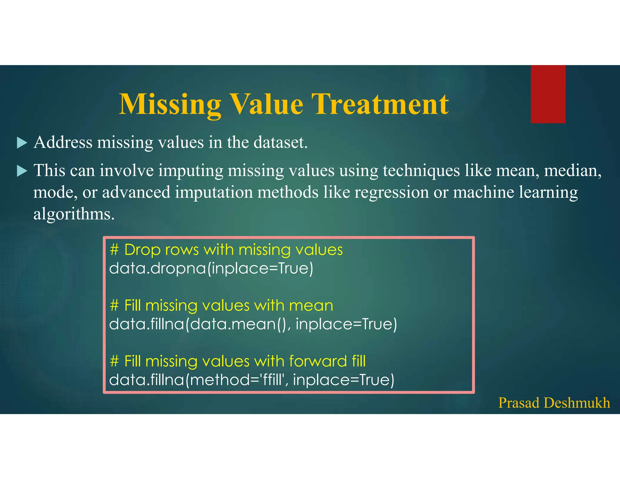
  Data Cleaning  Cleanthe data to ensure it is in a usable format.  This includes handling missing values, removing duplicates, correcting inconsistent data, and transforming data types if necessary. # Handling missing values data.dropna() # Drop rows with missing values data.fillna(value) # Fill missing values with a specific value # Removing duplicates data.drop_duplicates() # Correcting inconsistent data data['column_name'].replace(old_value, new_value, inplace=True) Prasad Deshmukh
• 6.
  Missing Value Treatment Address missing values in the dataset.  This can involve imputing missing values using techniques like mean, median, mode, or advanced imputation methods like regression or machine learning algorithms. # Drop rows with missing values data.dropna(inplace=True) # Fill missing values with mean data.fillna(data.mean(), inplace=True) # Fill missing values with forward fill data.fillna(method='ffill', inplace=True) Prasad Deshmukh
• 7.
  Summary Statistics  Computebasic summary statistics such as mean, median, mode, standard deviation, and quartiles for numerical variables.  For categorical variables, you can calculate frequency counts or proportions for each category. # Compute basic summary statistics data.describe() # Calculate mean, median, mode data.mean() data.median() data.mode() Prasad Deshmukh
• 8.
  Data Visualization  Createvisual representations of the data using graphs, charts, and plots.  This helps to identify patterns, trends, and outliers.  Common visualizations include histograms, box plots, scatter plots, bar charts, and heatmaps. import matplotlib.pyplot as plt import seaborn as sns # Histogram plt.hist(data['column_name']) # Box plot sns.boxplot(x=data['column_name']) # Scatter plot plt.scatter(data['x_column'], data['y_column']) # Bar chart sns.countplot(data['category_column']) # Heatmap sns.heatmap(data.corr()) Prasad Deshmukh
• 9.
  Correlation Analysis  Examinethe relationships between variables by calculating correlation coefficients.  This helps to identify variables that are highly correlated, positively or negatively, and can provide insights into potential predictors or multicollinearity. # Calculate correlation matrix correlation_matrix = data.corr() # Heatmap of correlation matrix sns.heatmap(correlation_matrix, annot=True, cmap='coolwarm') Prasad Deshmukh
• 10.
  Outlier Detection  Identifyand handle outliers in the data.  Outliers can significantly impact analysis results, so it's important to detect and understand their presence.  Common techniques for outlier detection include box plots, z-scores, and clustering methods. # Box plot sns.boxplot(x=data['column_name']) # Z-score method from scipy.stats import zscore data['z_score'] = zscore(data['column_name']) outliers = data[(data['z_score'] > 3) | (data['z_score'] < -3)] Prasad Deshmukh
• 11.
  Data Transformation  Performtransformations on variables to make the data more suitable for analysis or modeling.  Examples include log transformations, square roots, normalization, or standardization. # Log transformation data['log_transformed'] = np.log(data['column_name']) # Standardization from sklearn.preprocessing import StandardScaler scaler = StandardScaler() data['standardized_column'] = scaler.fit_transform(data['column_name'].values.reshape(-1, 1)) Prasad Deshmukh
• 12.
  Hypothesis Testing  Ifapplicable, conduct statistical tests to validate hypotheses or assumptions about the data.  This can involve t-tests, chi-square tests, ANOVA, or other appropriate tests based on the nature of the data and the research questions. from scipy.stats import ttest_ind # Perform t-test between two groups group1 = data[data['group'] == 1]['column_name'] group2 = data[data['group'] == 2]['column_name'] statistic, p_value = ttest_ind(group1, group2) Prasad Deshmukh
• 13.
  Iterative Analysis  EDAis often an iterative process.  As you uncover insights, you may go back and refine your analysis, perform additional transformations, or explore specific aspects in more detail. Prasad Deshmukh
• 14.
  In conclusion, ExploratoryData Analysis (EDA) is a crucial step in the data analysis process that helps to understand the dataset, identify patterns, relationships, and outliers, and inform subsequent analysis and modeling decisions. It provides valuable insights and serves as a foundation for data-driven decision-making. Prasad Deshmukh
• 15.
  THANK YOU Prasad Deshmukh