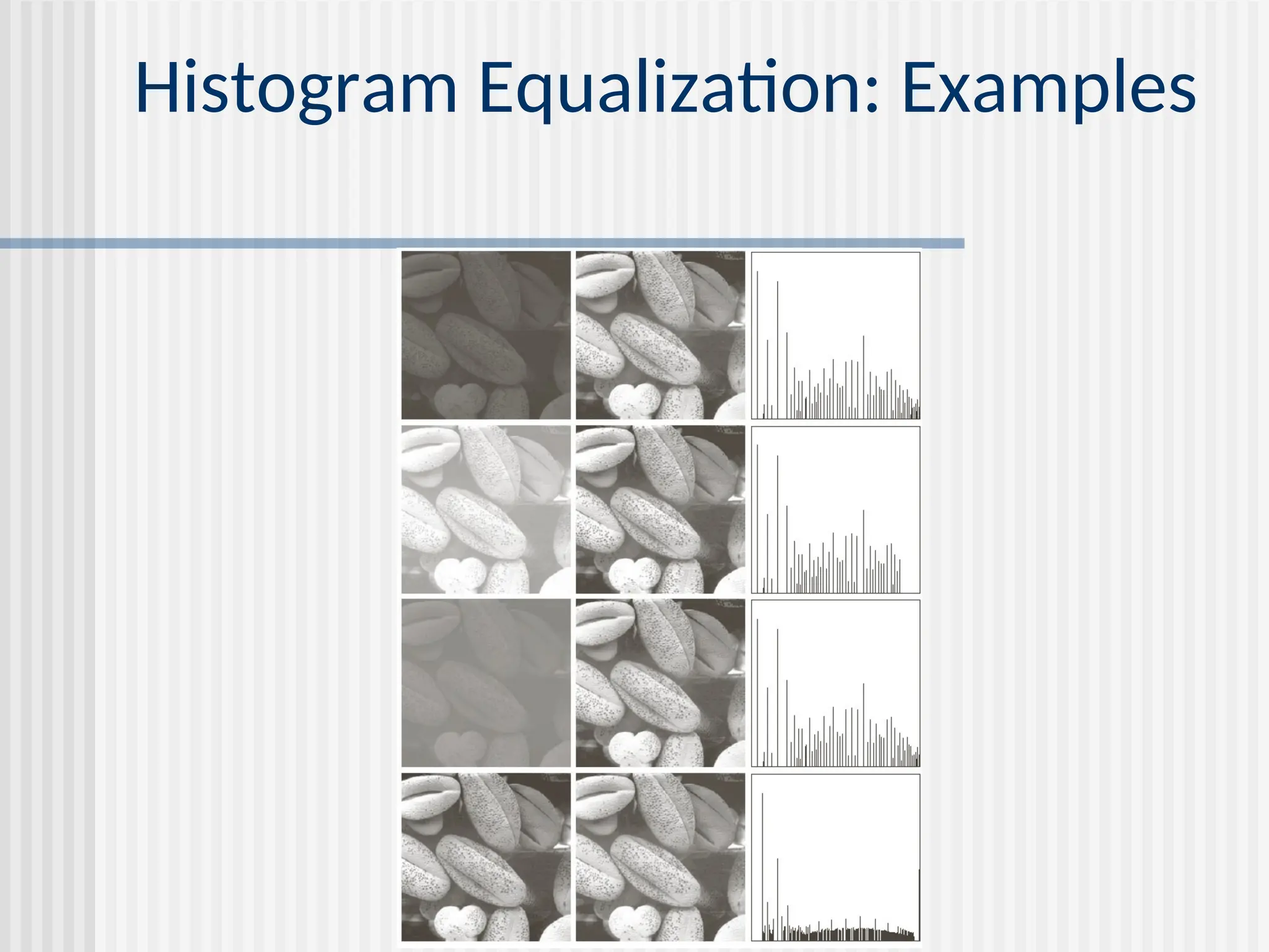
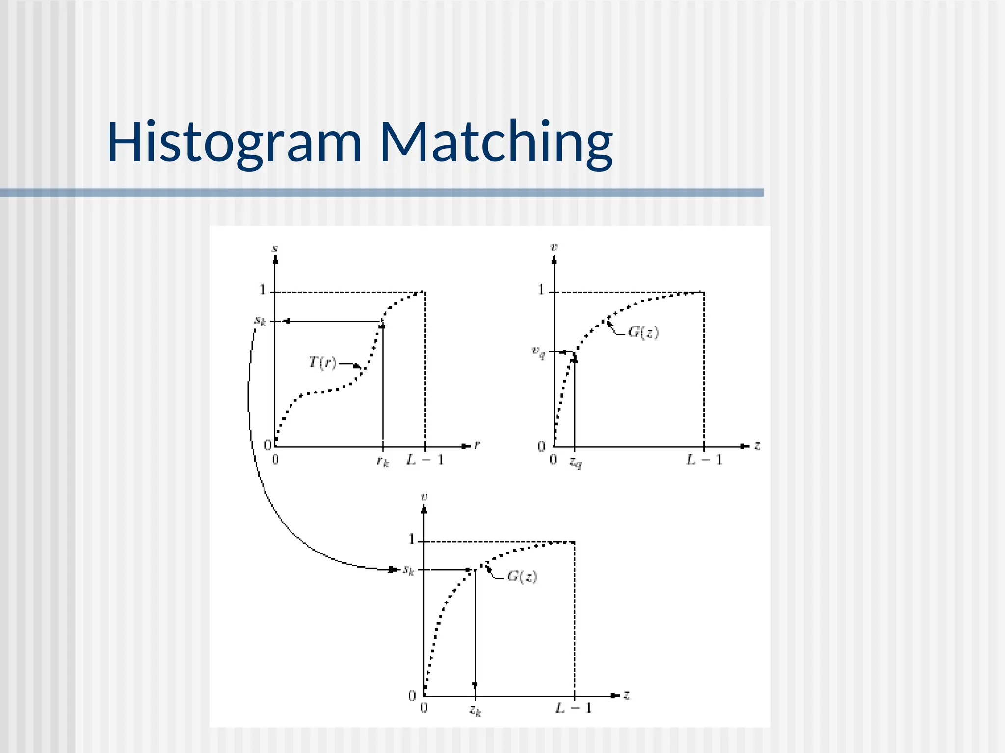
Digital Image Processing UNIT-2.ppt

Chapter 2 IMAGE ENHANCEMENT IN THE SPATIAL DOMAIN

Outline  Background  Basic Gray-level transformation  Histogram Processing  Arithmetic-Logic Operation  Basics of Spatial Filtering  Smoothing Spatial Filters  Sharpening Spatial Filters  Combining Spatial Enhancement Methods  Fuzzy techniques*

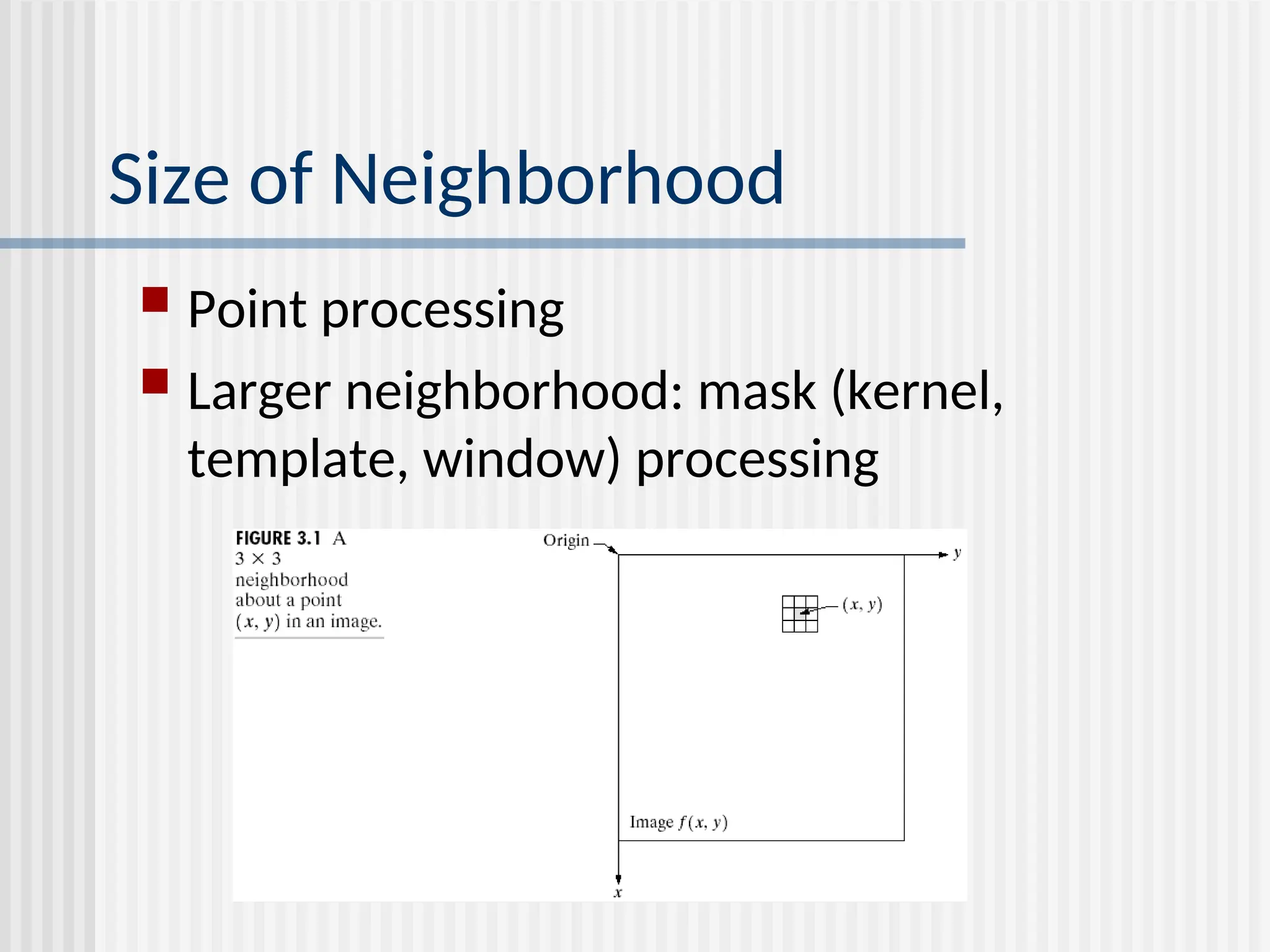
 Image enhancement approaches fall into two broad categories: spatial domain methods and frequency domain methods.  The term spatial domain refers to the image plane itself.  g(x,y)= T[f(x,y)] , T is an operator on f, defined over some neighborhood of f(x,y) Background

Size of Neighborhood  Point processing  Larger neighborhood: mask (kernel, template, window) processing

Gray-level Transformation Contrast stretching thresholding

Basic Gray Level Transformation  Image negatives: s =L-1-r  Log transformation: s =clog(1+r)  Power-law transformation: s=cr

Gamma Correction (I)  Cathode ray tube (CRT) devices have an intensity-to-voltage response that is a power function, with exponents varying from 1.8 to 2.5.  cr s   cr s 

Power-Law Transformation (I)  cr s 

Power-Law Transformation (II)  cr s 

Piece-wise Linear Transformation  Contrast stretching  Gray-level slicing (Figure 3.11,12)  Bit-plane slicing (Figures 3.13-15)

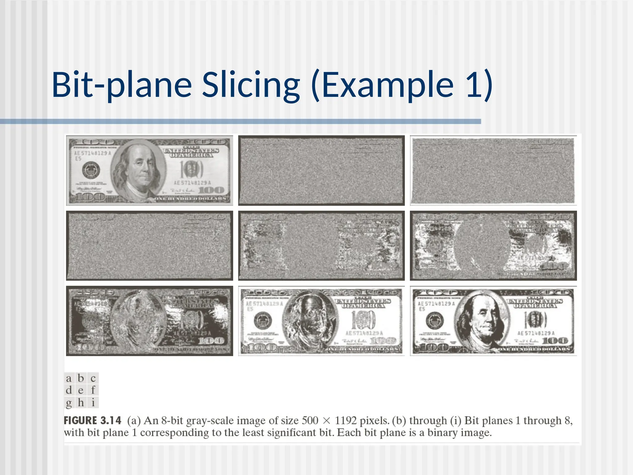
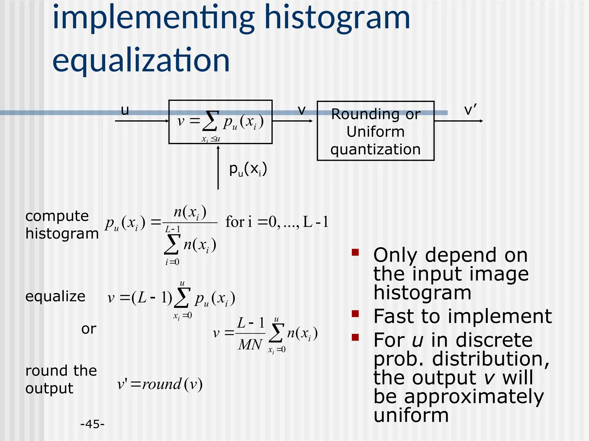
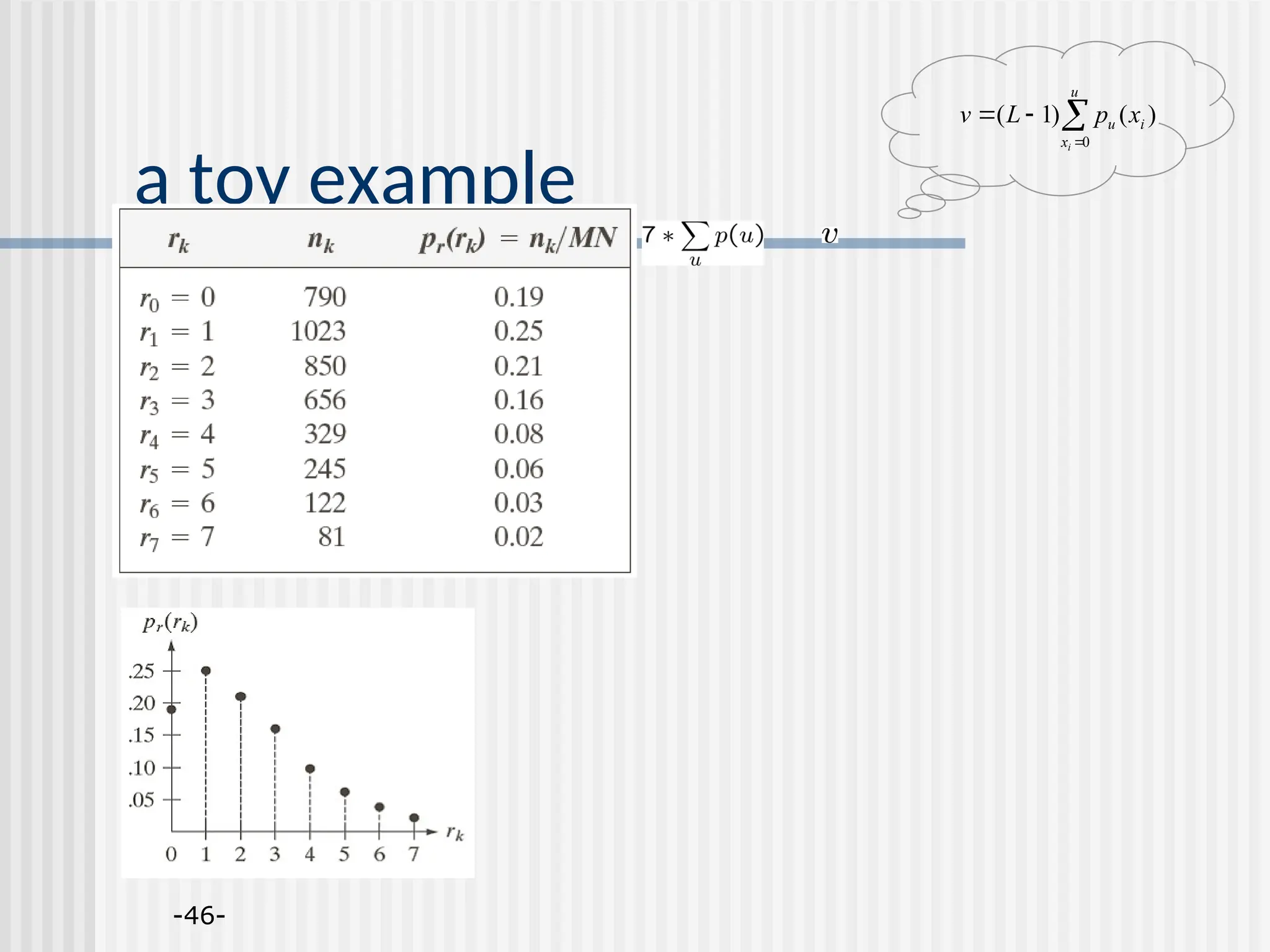
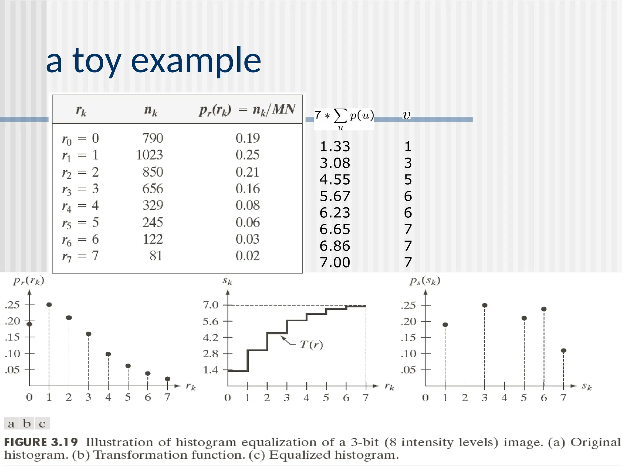
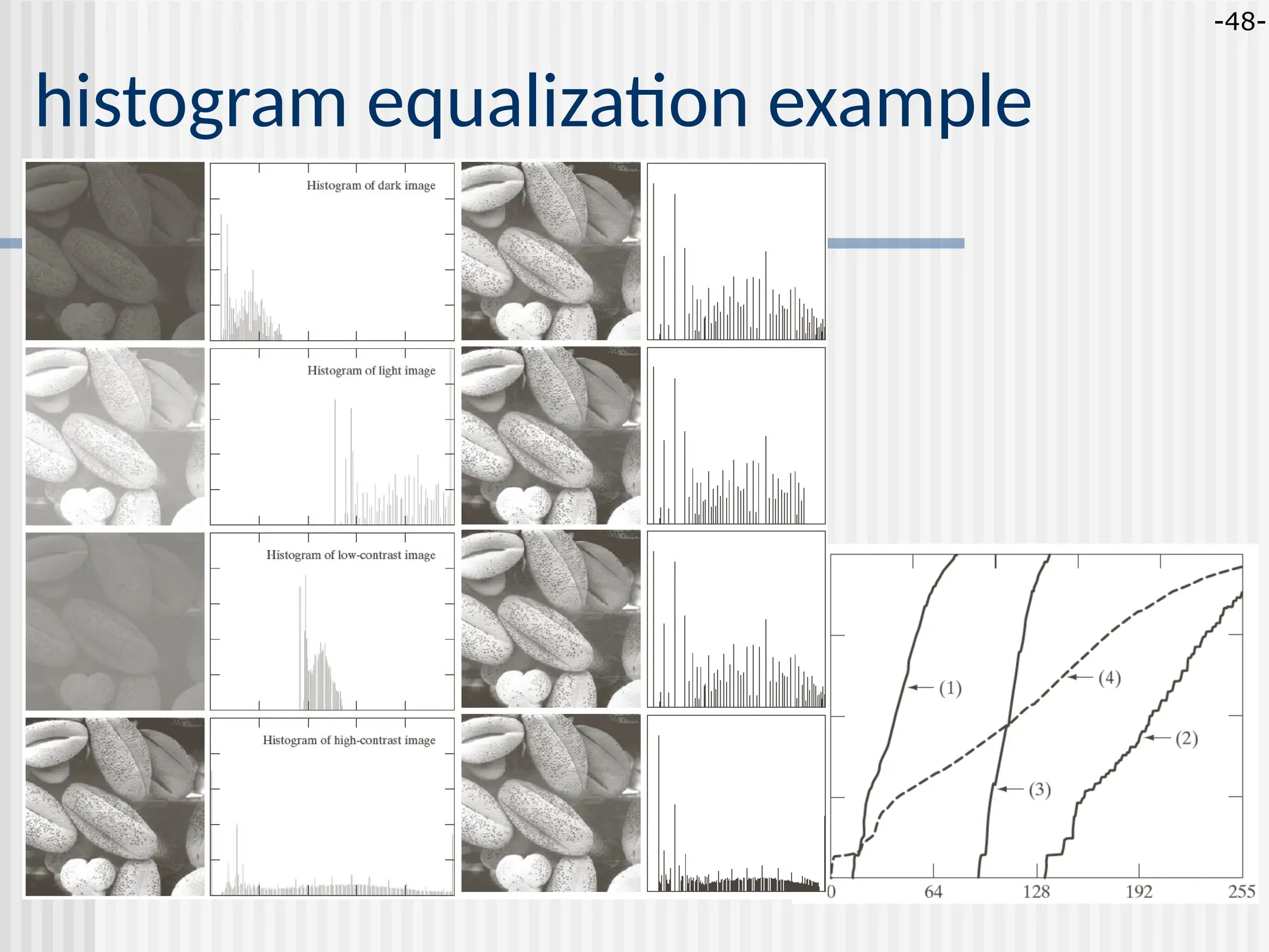
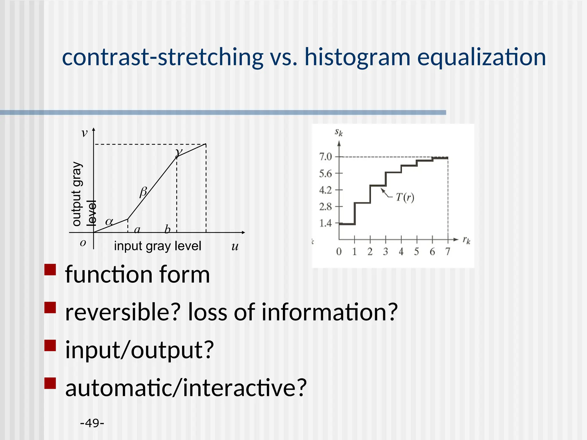
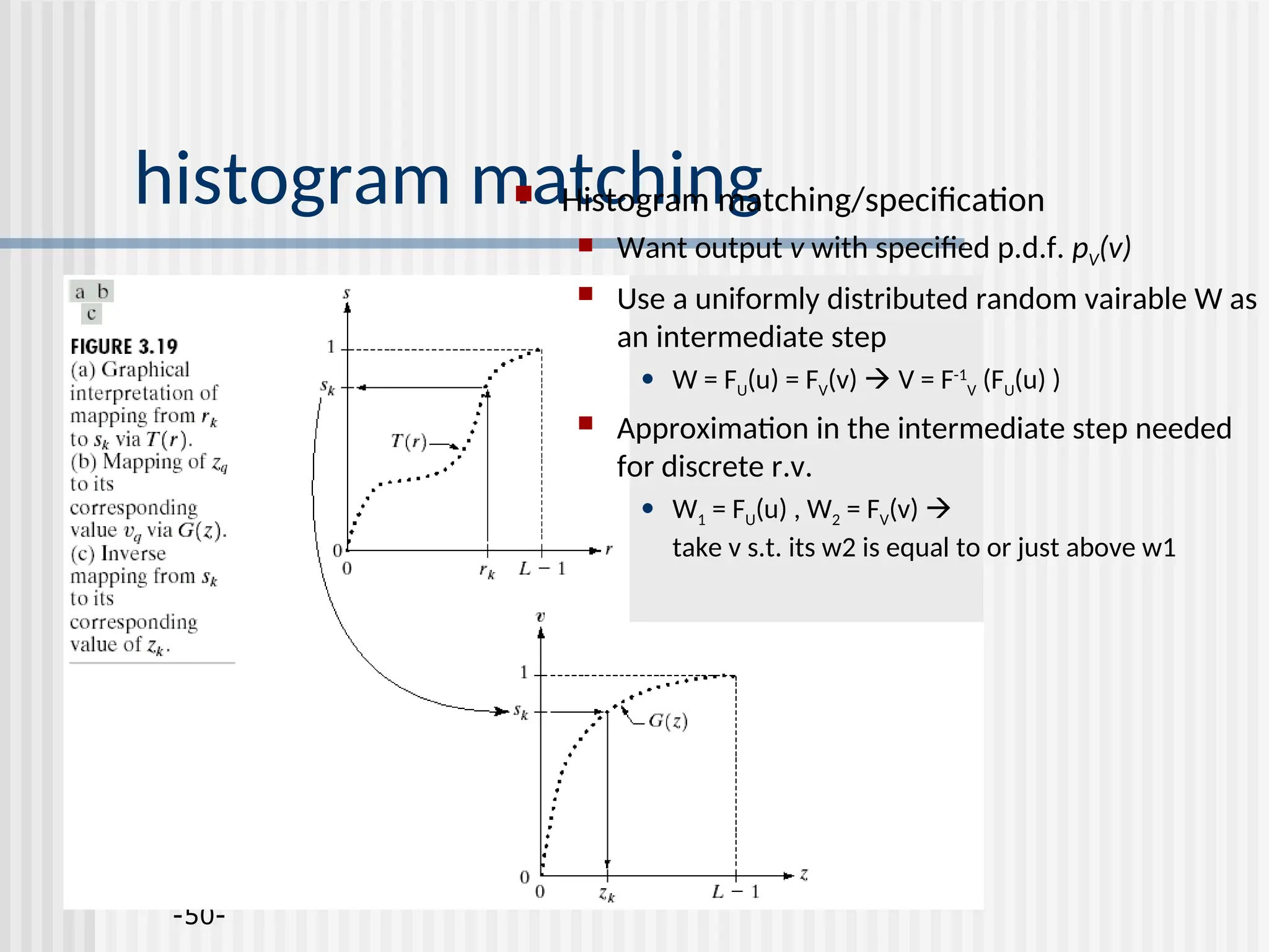
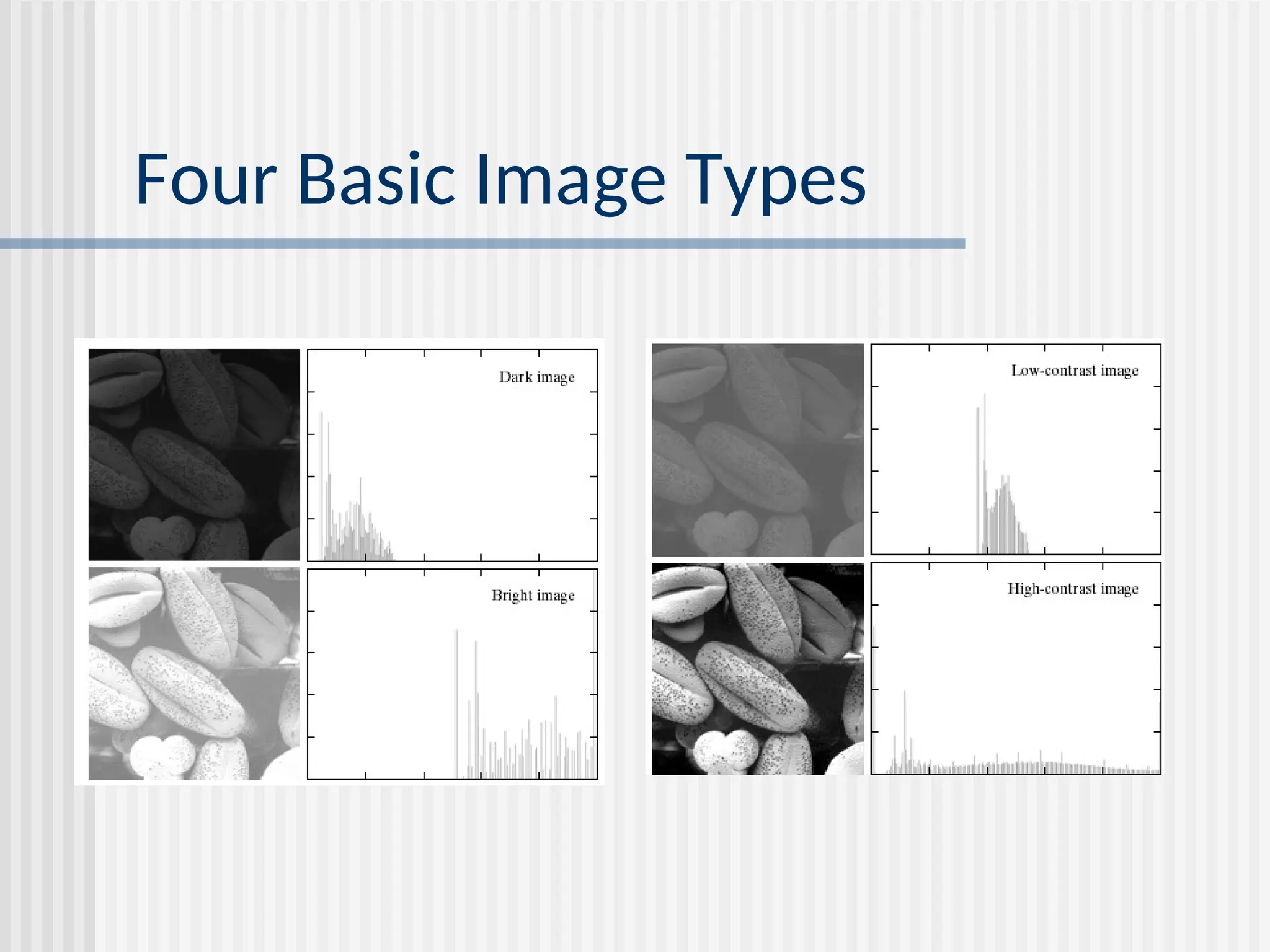
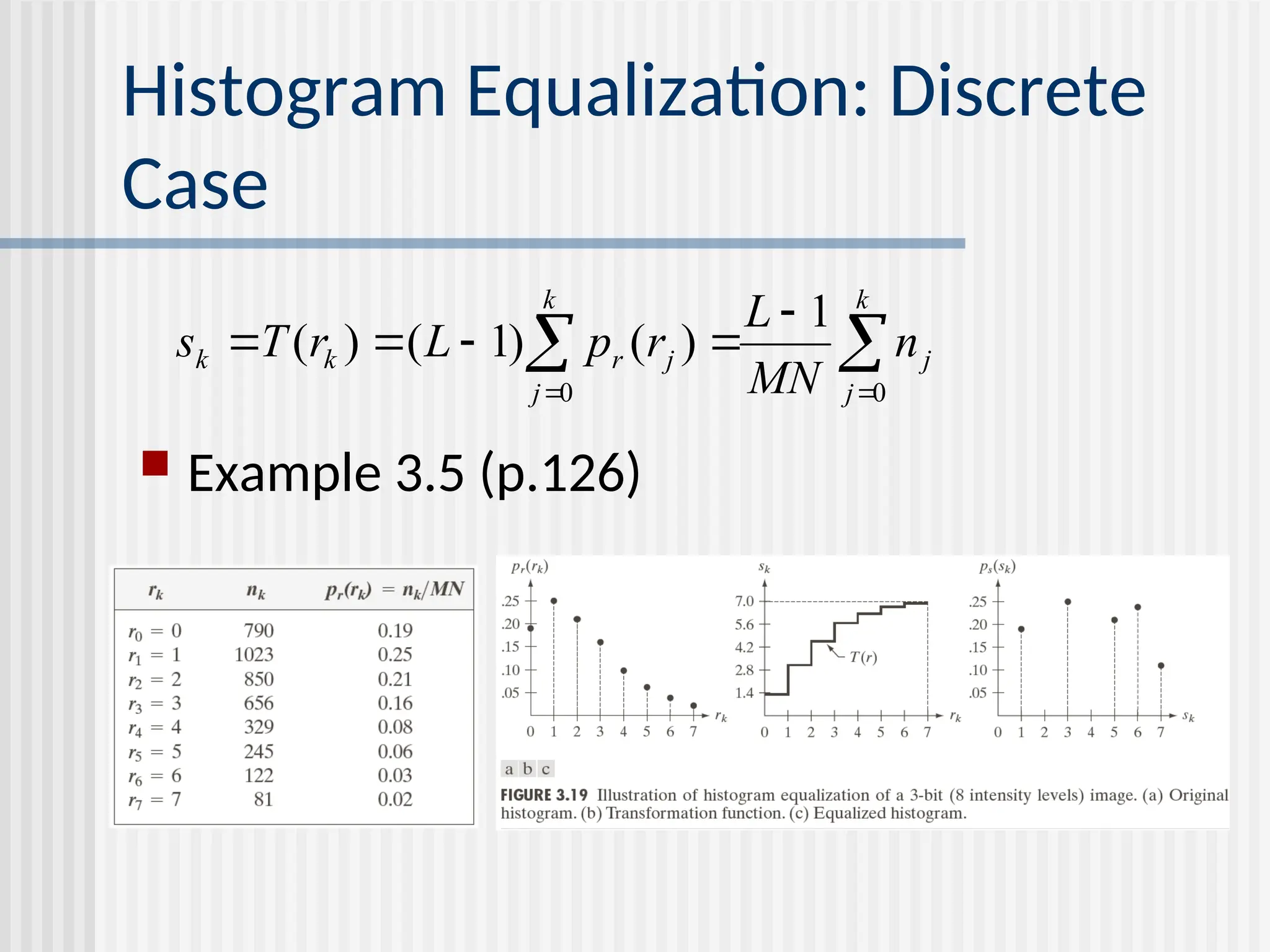
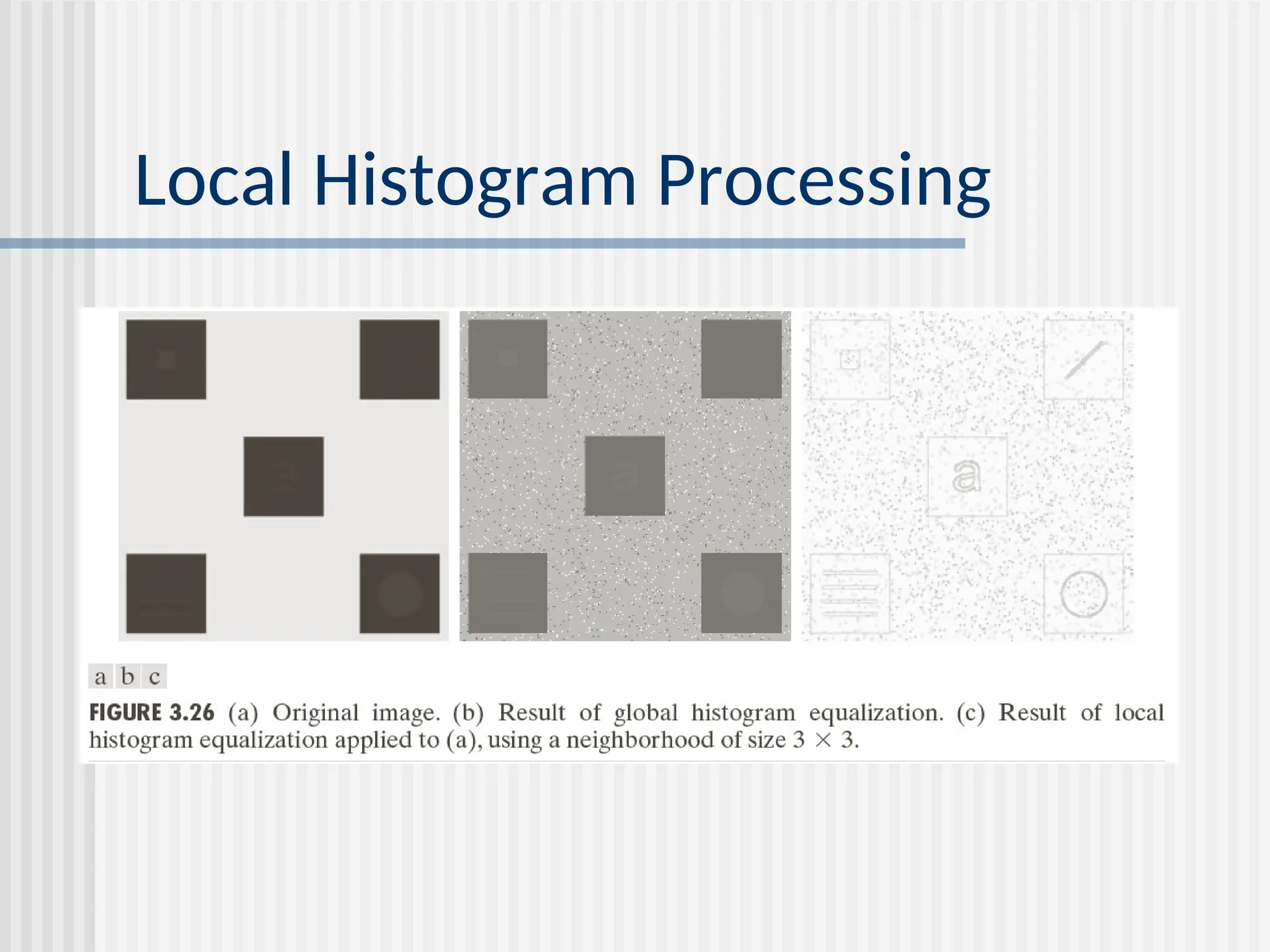
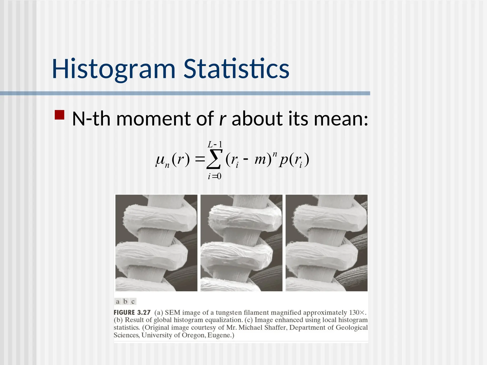
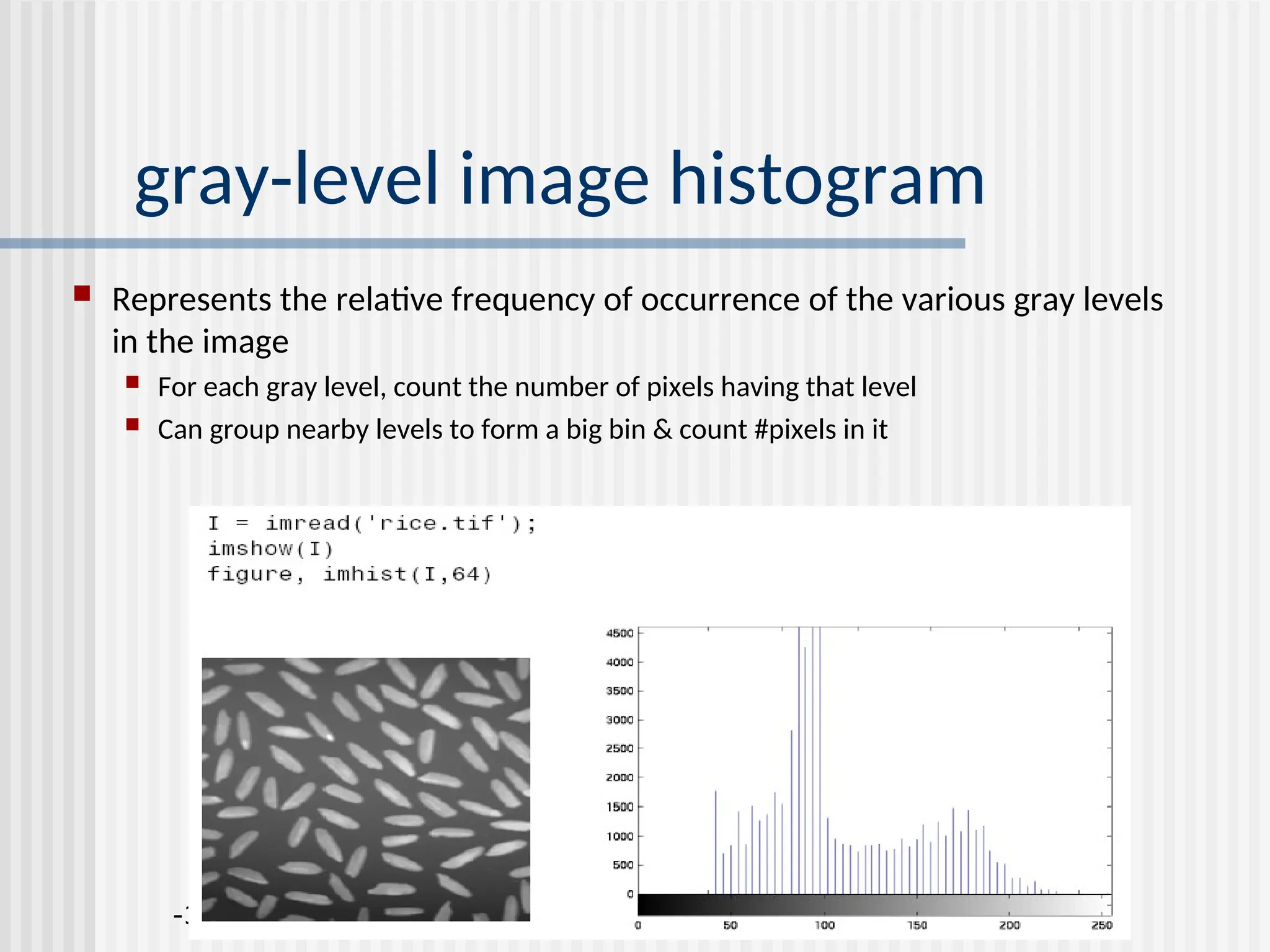
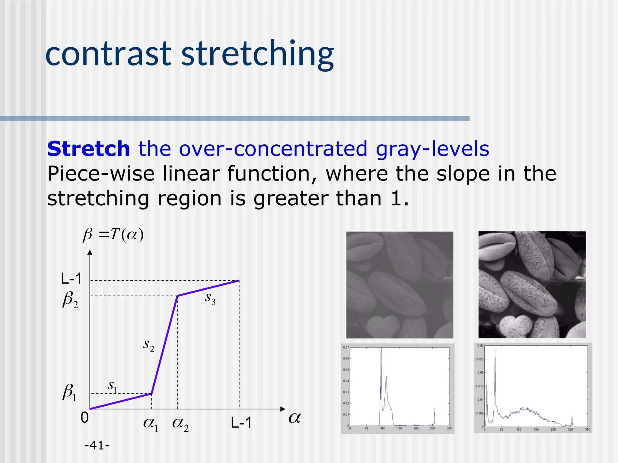
Histogram Processing  The histogram of a digital image with gray-levels in the range [0,L-1] is a discrete function h(rk)=nk where rk is the kth gray level and nk is the number of pixels in the image having gray level rk  Normalized histogram: p(rk)=nk/MN.  Easy to compute, good for real-time image processing.

Histogram Transformation   T(r) is a monotonically increasing function  1 0 ), (     L r r T s 1 0 for 1 ) ( 0       L r L r T

Histogram Equalization  What if we take the transformation T to be:  It can be shown that ps(s)=1/(L-1)  Example 3.4 (p.125)   d p L r T s r r ) ( ) 1 ( ) ( 0    

 Example 3.5 (p.126) Histogram Equalization: Discrete Case          k j j k j j r k k n MN L r p L r T s 0 0 1 ) ( ) 1 ( ) (

Histogram Equalization: Examples

Histogram Statistics  N-th moment of r about its mean: ) ( ) ( ) ( 1 0 i L i n i n r p m r r      

Arithmetic Operations  Image Subtraction  Image Averaging

Basics of Spatial Filtering •Mask, convolution kernels •Odd sizes

Spatial Correlation and Convolution           b b t a a s t y s x f t s w y x f y x w ) , ( ) , ( ) , ( ) , (           b b t a a s t y s x f t s w y x f y x w ) , ( ) , ( ) , ( ) , ( Correlation Convolution

Smoothing Spatial Filters  Smoothing linear filters: averaging filters, low-pass filters  Box filter  Weighted average  Order-statistics filters:  Median-filter: removing salt-and-pepper noise  Max filter  Min filter

Sharpening Spatial Filters  Foundation: ) ( 2 ) 1 ( ) 1 ( ) ( ) 1 ( 2 2 x f x f x f x f x f x f x f            

The Laplacian  Development of the method: ) , ( 4 ) 1 , ( ) 1 , ( ) , 1 ( ) , 1 ( ) , ( 2 ) 1 , ( ) 1 , ( ) , ( 2 ) , 1 ( ) , 1 ( 2 2 2 2 2 2 2 2 2 2 y x f y x f y x f y x f y x f f y x f y x f y x f y f y x f y x f y x f x f y f x f f                               

Combining Spatial Enhancement Methods (a) original (b) Laplacian, (c) a+b, (d) Sobel of (a) (a) (b) (c) (d)

-39- gray-level image histogram  Represents the relative frequency of occurrence of the various gray levels in the image  For each gray level, count the number of pixels having that level  Can group nearby levels to form a big bin & count #pixels in it

-40- interpretations of histogram  if pixel values are i.i.d random variables  histogram is an estimate of the probability distribution of the r.v.  “unbalanced” histograms do not fully utilize the dynamic range  Low contrast image: narrow luminance range  Under-exposed image: concentrating on the dark side  Over-exposed image: concentrating on the bright side  “balanced” histogram gives more pleasant look and reveals rich details

-41- contrast stretching  ) (  T  2  1  2  1  0 L-1 1 s 2 s 3 s L-1 Stretch the over-concentrated gray-levels Piece-wise linear function, where the slope in the stretching region is greater than 1.

-42- … in practice  intuition about a “good” image:  a “uniform” histogram spanning a large variety of gray tones  can we figure out a stretching function automatically?

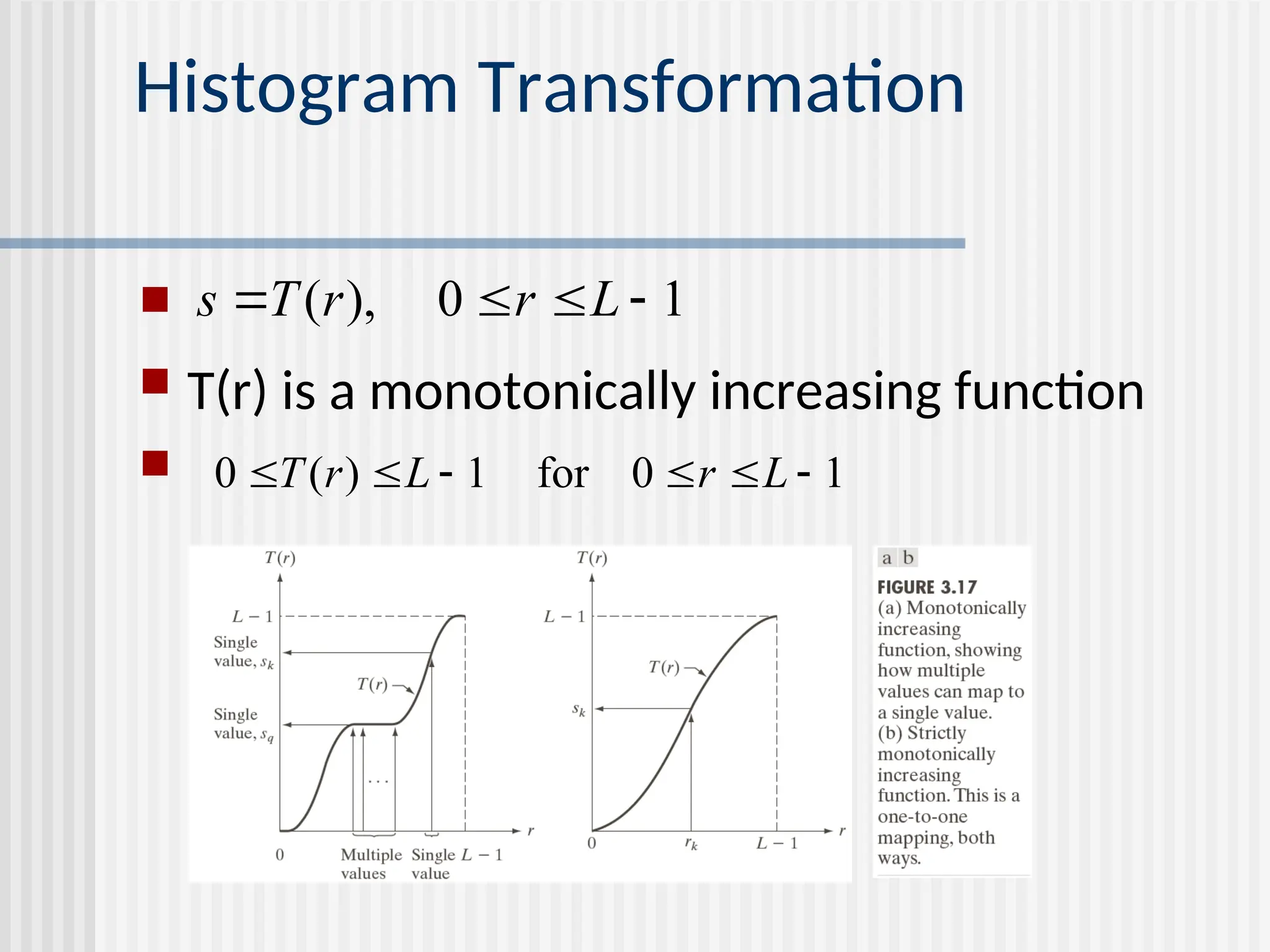
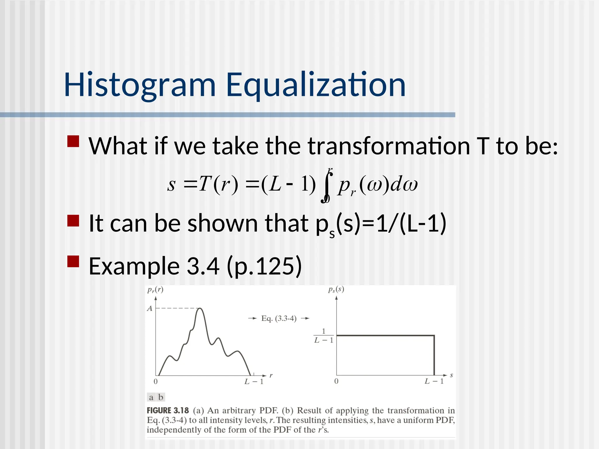
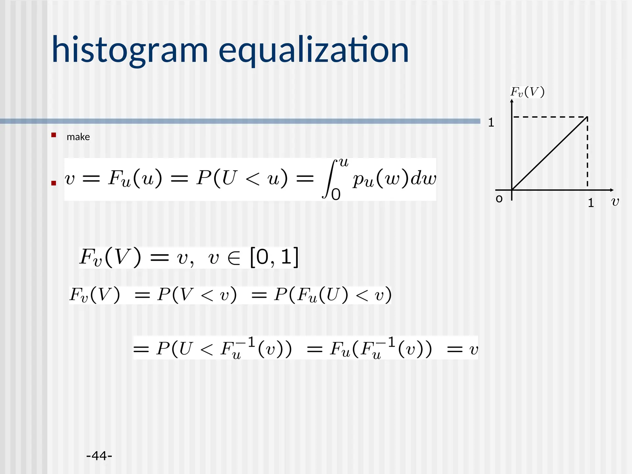
-43- histogram equalization  goal: map the each luminance level to a new value such that the output image has approximately uniform distribution of gray levels  two desired properties  monotonic (non-decreasing) function: no value reversals  [0,1][0.1] : the output range being the same as the input range pdf cdf o 1 1 o 1 1

-44- histogram equalization  make  show o 1 1

-45- implementing histogram equalization 1 - L ..., 0, i for ) ( ) ( ) ( 1 0      L i i i i u x n x n x p     u x i u i x p L v 0 ) ( ) 1 ( ) ( ' v round v     u x i u i x p v ) ( Rounding or Uniform quantization u v v’ pu(xi)  Only depend on the input image histogram  Fast to implement  For u in discrete prob. distribution, the output v will be approximately uniform compute histogram equalize round the output     u x i i x n MN L v 0 ) ( 1 or

-46- a toy example     u x i u i x p L v 0 ) ( ) 1 (

-47- a toy example 1.33 3.08 4.55 5.67 6.23 6.65 6.86 7.00 1 3 5 6 6 7 7 7

-48- histogram equalization example

-49- contrast-stretching vs. histogram equalization  function form  reversible? loss of information?  input/output?  automatic/interactive? input gray level u output gray level v a b o   

-50- histogram matching  Histogram matching/specification  Want output v with specified p.d.f. pV(v)  Use a uniformly distributed random vairable W as an intermediate step • W = FU(u) = FV(v)  V = F-1 V (FU(u) )  Approximation in the intermediate step needed for discrete r.v. • W1 = FU(u) , W2 = FV(v)  take v s.t. its w2 is equal to or just above w1

-51- histogram matching example

-52- local histogram processing  problem: global spatial processing not always desirable  solution: apply point-operations to a pixel neighborhood with a sliding window

-53- spatial filtering in image neighborhoods

-54- kernel operator / filter masks Spatial Filtering f g (.) (.) w TN           a a i b b j j n i m f j i w n m g ) , ( ) , ( ) , ( N n M m     1 1 kernel

-55- Smoothing: Image Averaging Low-pass filter, leads to softened edges smoothing operator

-56- spatial averaging can suppress noise  image with iid noise y(m,n) = x(m,n) + N(m,n)  averaging v(m,n) = (1/Nw)  x(m-k, n-l) + (1/Nw)  N(m-k, n-l) • Nw: number of pixels in the averaging window  Noise variance reduced by a factor of Nw  SNR improved by a factor of Nw  Window size is limited to avoid excessive blurring UMCP ENEE408G Slides (created by M.Wu & R.Liu © 2002)

-57- smoothing operator of different sizes 3x3 5x5 15x15 9x9 35x35 original

-58- directional smoothing  Problems with simple spatial averaging mask  Edges get blurred  Improvement  Restrict smoothing to along edge direction  Avoid filtering across edges  Directional smoothing  Compute spatial average along several directions  Take the result from the direction giving the smallest changes before & after filtering  Other solutions  Use more explicit edge detection and adapt filtering accordingly  W UMCP ENEE408G Slides (created by M.Wu & R.Liu © 2002)

-59- non-linear smoothing operator  Median filtering  median value  over a small window of size Nw  nonlinear • median{ x(m) + y(m) }  median{x(m)} + median{y(m)}  odd window size is commonly used • 3x3, 5x5, 7x7 • 5-pixel “+”-shaped window  for even-sized windows take the average of two middle values as output  Other order statistics: min, max, x-percentile …

-60- median filter example iid noise more at lecture 7, “image restoration”  Median filtering  resilient to statistical outliers  incurs less blurring  simple to implement

-61- image derivative and sharpening

-62- edge and the first derivative  Edge: pixel locations of abrupt luminance change  Spatial luminance gradient vector  a vector consists of partial derivatives along two orthogonal directions  gradient gives the direction with highest rate of luminance changes  Representing edge: edge intensity + directions  Detection Methods  prepare edge examples (templates) of different intensities and directions, then find the best match  measure transitions along 2 orthogonal directions

-63- edge detection operators Robert’s operato r Sobel’s operato r                          y f x f G G f y x Image gradient: y x G G f   

-64- edge detection example http://flickr.com/photos/reneemarie11/97326485/ Roberts Sobel

-65- second derivative in 2D Image Laplacian:

-66- laplacian of roman ruins http://flickr.com/photos/starfish235/388557119/

-67- unsharp masking  Unsharp masking is an image manipulation technique for increasing the apparent sharpness of photographic images.  The "unsharp" of the name derives from the fact that the technique uses a blurred, or "unsharp", positive to create a "mask" of the original image. The unsharped mask is then combined with the negative, creating a resulting image sharper than the original.  Steps  Blur the image  Subtract the blurred version from the original (this is called the mask)  Add the “mask” to the original

-68- high-boost filtering Avg. + + - ) , ( ) , ( ) , ( y x f y x Af y x f lp hb   Unsharp mask: high-boost with A=1

Spring 2012 Meetings 5 and 6, 7:20PM- 10PM FUZZY SET, MEMBERSHIP FUCTION, OPERATIONS Figure 1. Input output membership functions. Digital Image Processing, 3rd Ed, by R.C. Gonzalez, Richard, Prentice Hull 2007

Spring 2012 Meetings 5 and 6, 7:20PM- 10PM Fuzzy rule based system Figure 2. The basic steps of a fuzzy rule based system Digital Image Processing, 3rd Ed, by R.C. Gonzalez, Richard, Prentice Hull 2007

Spring 2012 Meetings 5 and 6, 7:20PM- 10PM Fuzzy Algorithms The calculation complexity of the five steps approach, introduced above, includes fuzzifycation and defuzzifycation procedures, which are very time consuming. To speed up the algorithms a multi-variable single output function is often employed. As variables, this function may use multiple membership function. The results shown on the next slide are produced by using such a function which includes three membership functions, for: - dark, gray and white colors.

Spring 2012 Meetings 5 and 6, 7:20PM- 10PM Fuzzy Image Enhancement- Results Figure 3. Fuzzy contrast enhancement using a single output multi-variable function, which includes dark, bright and gray color membership functions. Digital Image Processing, 3rd Ed, by R.C. Gonzalez, Richard, Prentice Hull 2007

Digital Image Processing UNIT-2.ppt

More Related Content

Similar to Digital Image Processing UNIT-2.ppt

More from durgakru

Recently uploaded

Digital Image Processing UNIT-2.ppt

Editor's Notes