Download as PDF, PPTX
![Pipeline Dataset creation #2a : Multiframe Techniques Note! In deep learning, the term super-resolution refers to “statistical upsampling” whereas in optical imaging super-resolution typically refers to imaging techniques. Note2! Nothing should stop someone marrying them two though In practice anyone can play with super-resolution at home by putting a camera on a tripod and then taking multiple shots of the same static scene, and post-processing them through super-resolution that can improve modulation transfer function (MTF) for RGB images, improve depth resolution and reduce noise for laser scans and depth sensing e.g. with Kinect. https://doi.org/10.2312/SPBG/SPBG06/009-015 Cited by 47 articles (a) One scan. (b) Final super-resolved surface from 100 scans. “PhotoAcute software processes sets of photographs taken in continuous mode. It utilizes superresolution algorithms to convert a sequence of images into a single high-resolution and low-noise picture, that could only be taken with much better camera.” Depth looks a lot nicer when reconstructed using 50 consecutive Kinec v1 frames in comparison to just one frame. [Data from Petteri Teikari[ Kinect multiframe reconstruction with SiftFu [Xiao et al. (2013)] https://github.com/jianxiongxiao/ProfXkit](https://image.slidesharecdn.com/datasetmultiviewcreation-170822074203/75/Dataset-creation-for-Deep-Learning-based-Geometric-Computer-Vision-problems-5-2048.jpg)
![Pipeline acquisition example with Kinect https://arxiv.org/abs/1704.07632 KinectFusion (Newcombe et al. 2011), one of the pioneering works, showed that a real-world object as well as an indoor scene canbe reconstructed in real-time with GPU acceleration. It exploits the iterative closest point (ICP) algorithm (Besl and McKay 1992) to track 6-DoF poses and the volumetric surface representation scheme with signed distance functions (Curless and Levoy, 1996) to fuse 3D measurements. A number of following studies (e.g. Choi et al. 2015) have tackled the limitation of KinectFusion; as the scale ofa scene increases, it is hard to completely reconstruct thescene due to the drift problem of the ICP algorithm as wellas the large memory consumption of volumetric integration. To scale up the KinectFusion algorithm, Whelan et al . (2012)] presented a spatially extended KinectFusion, named as Kintinuous, by incrementally adding KinectFusion results as the form of triangular meshes. Whelan et al . (2015) also proposed ElasticFusion to tackle similar problems as well as to overcome the problem of a pose graph optimization by using the surface loop closure optimization and the surfel-based representation. Moreover, to decrease the space complexity, ElasticFusion deallocates invisible surfels from the memory; invisible surfels are allocated in the memory again only if they are likely to be visible in the near future.](https://image.slidesharecdn.com/datasetmultiviewcreation-170822074203/75/Dataset-creation-for-Deep-Learning-based-Geometric-Computer-Vision-problems-11-2048.jpg)
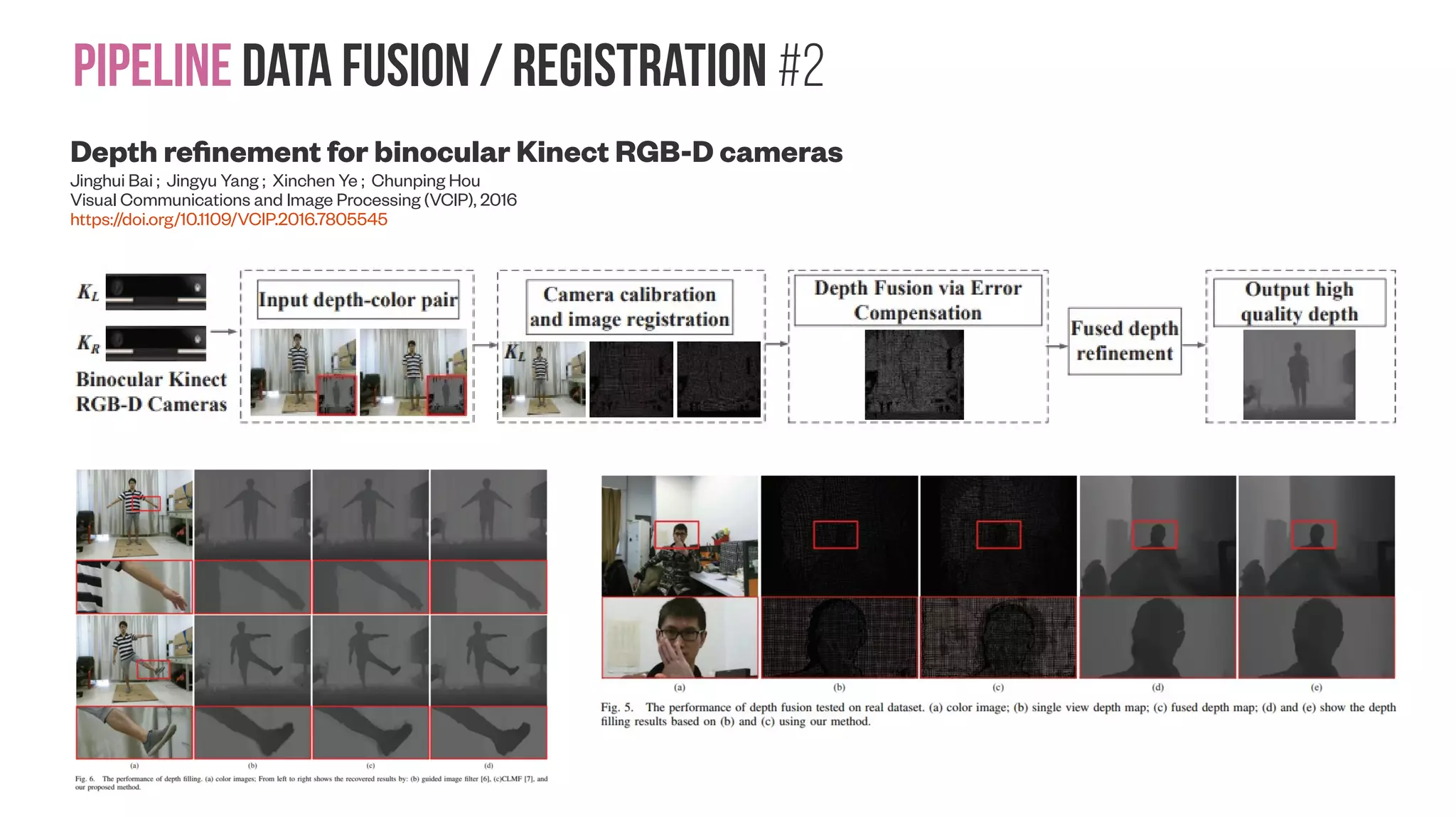
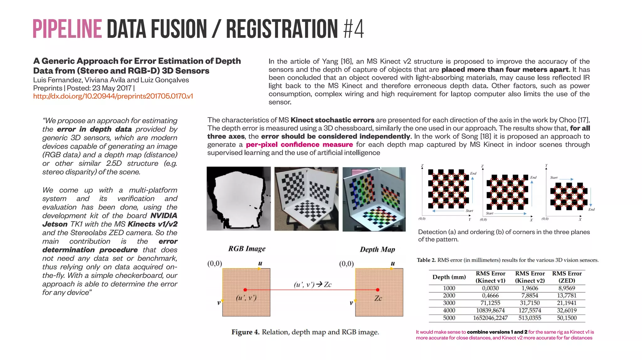
![Pipeline data Fusion / Registration #4 A Generic Approach for Error Estimation of Depth Data from (Stereo and RGB-D) 3D Sensors Luis Fernandez, Viviana Avila and Luiz Gonçalves Preprints | Posted: 23 May 2017 | http://dx.doi.org/10.20944/preprints201705.0170.v1 “We propose an approach for estimating the error in depth data provided by generic 3D sensors, which are modern devices capable of generating an image (RGB data) and a depth map (distance) or other similar 2.5D structure (e.g. stereo disparity) of the scene. We come up with a multi-platform system and its verification and evaluation has been done, using the development kit of the board NVIDIA Jetson TK1 with the MS Kinects v1/v2 and the Stereolabs ZED camera. So the main contribution is the error determination procedure that does not need any data set or benchmark, thus relying only on data acquired on- the-fly. With a simple checkerboard, our approach is able to determine the error for any device” In the article of Yang [16], an MS Kinect v2 structure is proposed to improve the accuracy of the sensors and the depth of capture of objects that are placed more than four meters apart. It has been concluded that an object covered with light-absorbing materials, may cause less reflected IR light back to the MS Kinect and therefore erroneous depth data. Other factors, such as power consumption, complex wiring and high requirement for laptop computer also limits the use of the sensor. The characteristics of MS Kinect stochastic errors are presented for each direction of the axis in the work by Choo [17]. The depth error is measured using a 3D chessboard, similarly the one used in our approach. The results show that, for all three axes, the error should be considered independently. In the work of Song [18] it is proposed an approach to generate a per-pixel confidence measure for each depth map captured by MS Kinect in indoor scenes through supervised learning and the use of artificial intelligence Detection (a) and ordering (b) of corners in the three planes of the pattern. It would make sense to combine versions 1 and 2 for the same rig as Kinect v1 is more accurate for close distances, and Kinect v2 more accurate for far distances](https://image.slidesharecdn.com/datasetmultiviewcreation-170822074203/75/Dataset-creation-for-Deep-Learning-based-Geometric-Computer-Vision-problems-18-2048.jpg)
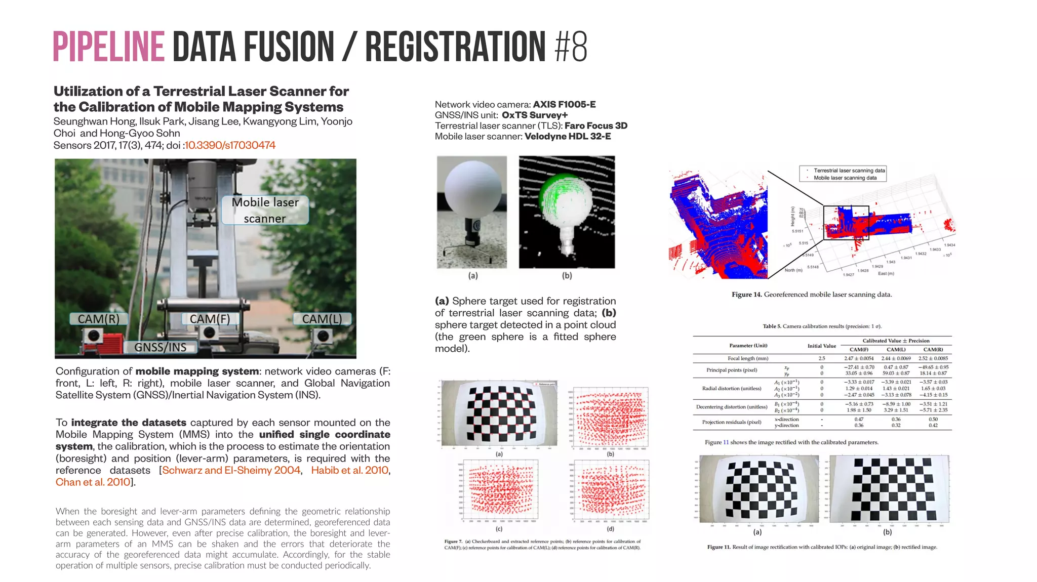
![Pipeline data Fusion / Registration #8 Utilization of a Terrestrial Laser Scanner for the Calibration of Mobile Mapping Systems Seunghwan Hong, Ilsuk Park, Jisang Lee, Kwangyong Lim, Yoonjo Choi and Hong-Gyoo Sohn Sensors 2017, 17(3), 474; doi :10.3390/s17030474 Configuration of mobile mapping system: network video cameras (F: front, L: left, R: right), mobile laser scanner, and Global Navigation Satellite System (GNSS)/Inertial Navigation System (INS). To integrate the datasets captured by each sensor mounted on the Mobile Mapping System (MMS) into the unified single coordinate system, the calibration, which is the process to estimate the orientation (boresight) and position (lever-arm) parameters, is required with the reference datasets [Schwarz and El-Sheimy 2004, Habib et al. 2010, Chan et al. 2010]. When the boresight and lever-arm parameters defining the geometric relationship between each sensing data and GNSS/INS data are determined, georeferenced data can be generated. However, even after precise calibration, the boresight and lever- arm parameters of an MMS can be shaken and the errors that deteriorate the accuracy of the georeferenced data might accumulate. Accordingly, for the stable operation of multiple sensors, precise calibration must be conducted periodically. (a) Sphere target used for registration of terrestrial laser scanning data; (b) sphere target detected in a point cloud (the green sphere is a fitted sphere model). Network video camera: AXIS F1005-E GNSS/INS unit: OxTS Survey+ Terrestrial laser scanner (TLS): Faro Focus 3D Mobile laser scanner: Velodyne HDL 32-E](https://image.slidesharecdn.com/datasetmultiviewcreation-170822074203/75/Dataset-creation-for-Deep-Learning-based-Geometric-Computer-Vision-problems-22-2048.jpg)

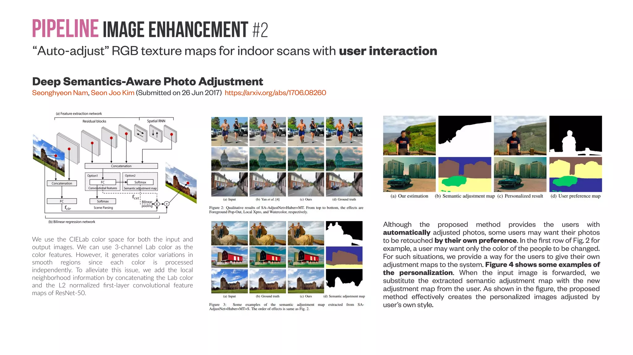
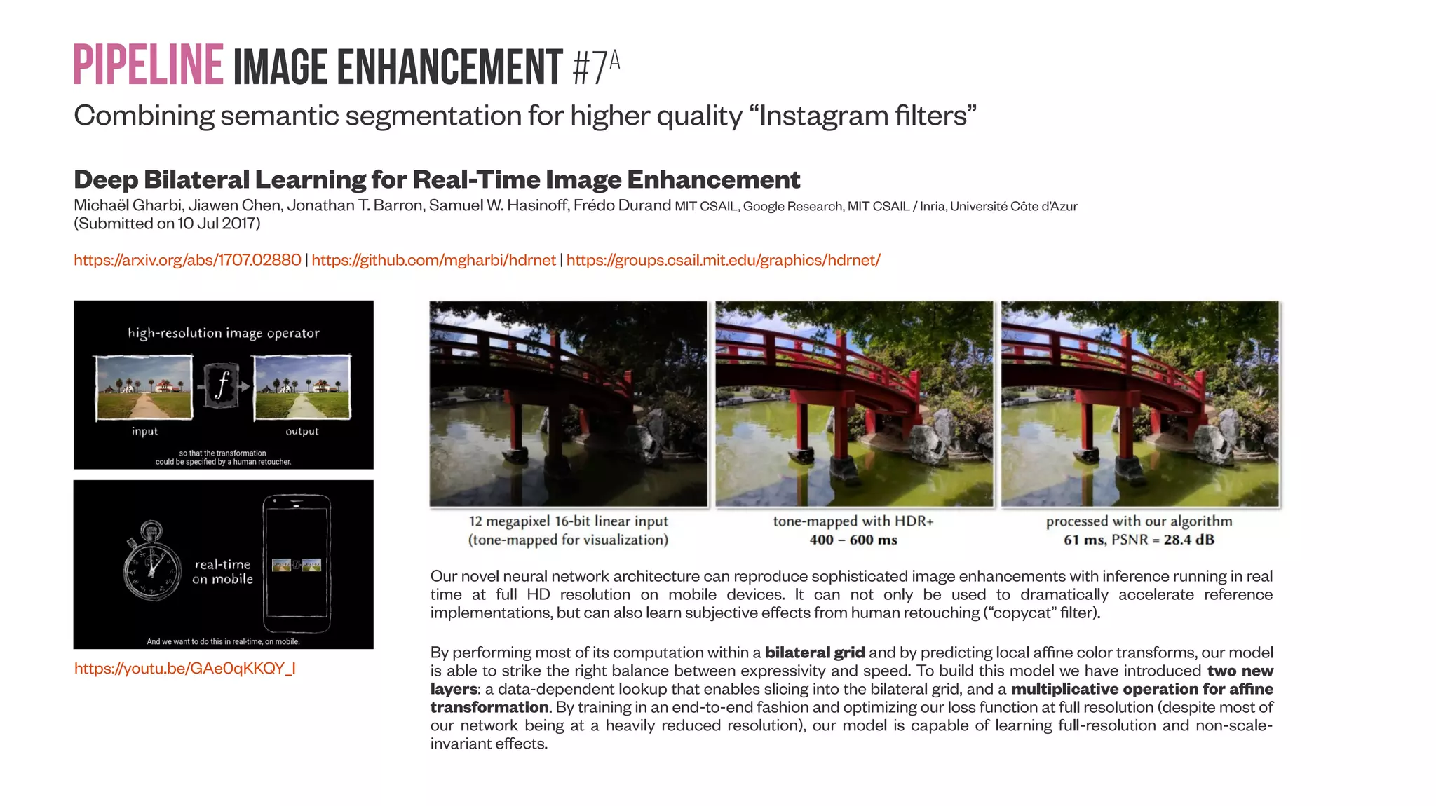
![Pipelineimage enhancement #4 “Auto-adjust” RGB texture maps for indoor scans with GANs for “auto-matting” Creatism: A deep-learning photographer capable of creating professional work Hui Fang, Meng Zhang (Submitted on 11 Jul 2017) https://arxiv.org/abs/1707.03491 https://google.github.io/creatism/ Datasets were created that contain ratings of photographs based on aesthetic quality [Murray et al., 2012] [Kong et al., 2016] [Lu et al., 2015]. Using our system, we mimic the workflow of a landscape photographer, from framing for the best composition to carrying out various post-processing operations. The environment for our virtual photographer is simulated by a collection of panorama images from Google Street View. We design a "Turing- test"-like experiment to objectively measure quality of its creations, where professional photographers rate a mixture of photographs from different sources blindly. We work with professional photographers to empirically de- fine 4 levels of aesthetic quality: ● 1: point-and-shoot photos without consideration. ● 2: Good photos from the majority of population without art background. Nothing artistic stands out. ● 3: Semi-pro. Great photos showing clear artistic aspects. The photographer is on the right track of becoming a professional. ● 4: Pro-work. Clearly each professional has his/her unique taste that needs calibration. We use AVA dataset [Murray et al., 2012] wto bootstrap a consensus among them. Assume there exists a universal aesthetics metric, Φ. By definition, needs to incorporate all aesthetic aspects, suchΦ as saturation, detail level, composition... To define withΦ examples, number of images needs to grow exponentially to cover more aspects [Jaroensri et al., 2015]. To make things worse, unlike traditional problems such as object recognition, what we need are not only natural images, but also pro- level photos, which are much less in quantity.](https://image.slidesharecdn.com/datasetmultiviewcreation-170822074203/75/Dataset-creation-for-Deep-Learning-based-Geometric-Computer-Vision-problems-33-2048.jpg)

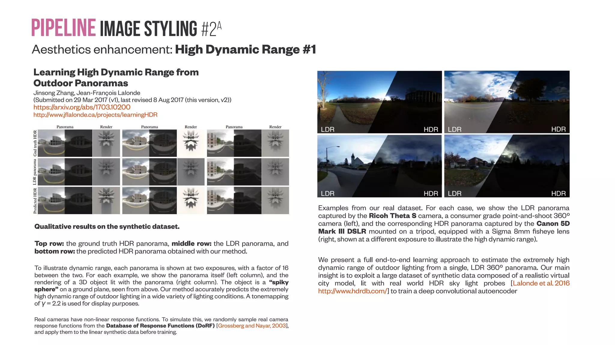
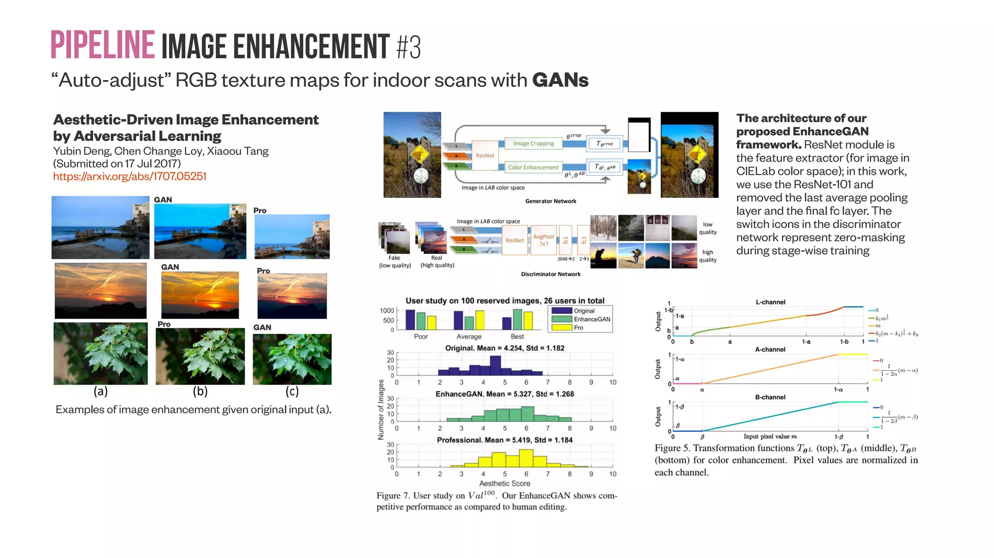
![Pipelineimage Styling #2A Aesthetics enhancement: High Dynamic Range #1 Learning High Dynamic Range from Outdoor Panoramas Jinsong Zhang, Jean-François Lalonde (Submitted on 29 Mar 2017 (v1), last revised 8 Aug 2017 (this version, v2)) https://arxiv.org/abs/1703.10200 http://www.jflalonde.ca/projects/learningHDR Qualitative results on the synthetic dataset. Top row: the ground truth HDR panorama, middle row: the LDR panorama, and bottom row: the predicted HDR panorama obtained with our method. To illustrate dynamic range, each panorama is shown at two exposures, with a factor of 16 between the two. For each example, we show the panorama itself (left column), and the rendering of a 3D object lit with the panorama (right column). The object is a “spiky sphere” on a ground plane, seen from above. Our method accurately predicts the extremely high dynamic range of outdoor lighting in a wide variety of lighting conditions. A tonemapping of γ = 2.2 is used for display purposes. Real cameras have non-linear response functions. To simulate this, we randomly sample real camera response functions from the Database of Response Functions (DoRF) [Grossberg and Nayar, 2003], and apply them to the linear synthetic data before training. Examples from our real dataset. For each case, we show the LDR panorama captured by the Ricoh Theta S camera, a consumer grade point-and-shoot 360º camera (left), and the corresponding HDR panorama captured by the Canon 5D Mark III DSLR mounted on a tripod, equipped with a Sigma 8mm fisheye lens (right, shown at a different exposure to illustrate the high dynamic range). We present a full end-to-end learning approach to estimate the extremely high dynamic range of outdoor lighting from a single, LDR 360º panorama. Our main insight is to exploit a large dataset of synthetic data composed of a realistic virtual city model, lit with real world HDR sky light probes [Lalonde et al. 2016 http://www.hdrdb.com/] to train a deep convolutional autoencoder](https://image.slidesharecdn.com/datasetmultiviewcreation-170822074203/75/Dataset-creation-for-Deep-Learning-based-Geometric-Computer-Vision-problems-40-2048.jpg)
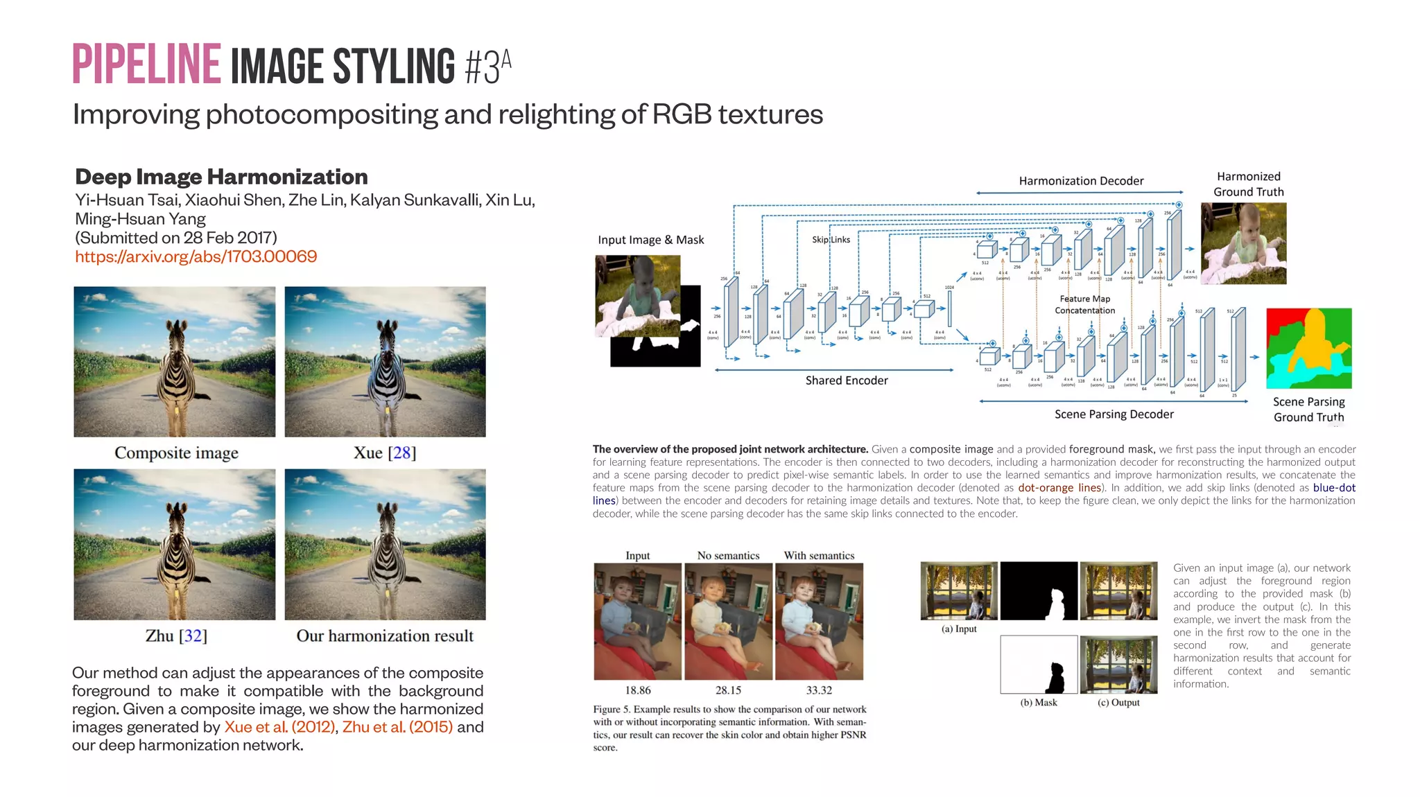
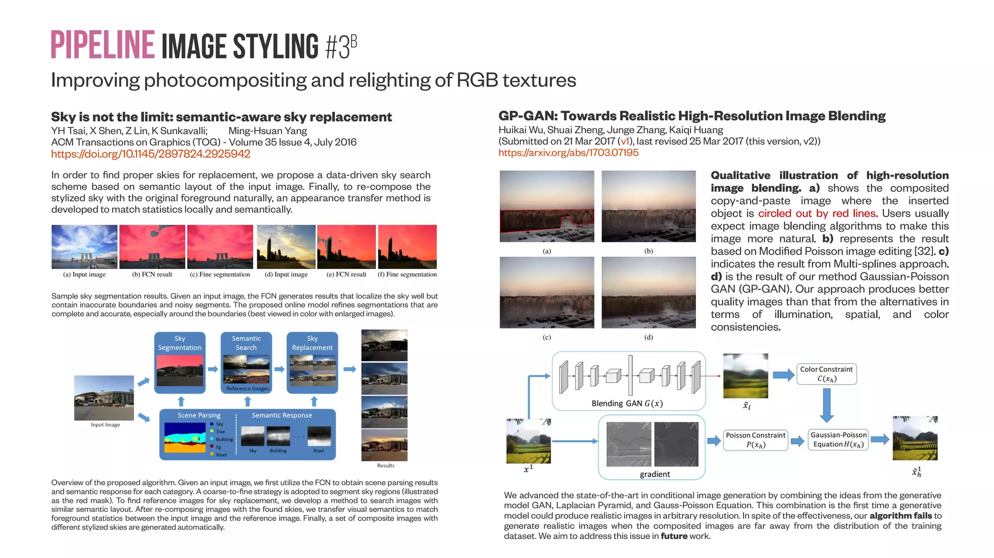
![Pipelineimage Styling #3b Sky is not the limit: semantic-aware sky replacement YH Tsai, X Shen, Z Lin, K Sunkavalli; Ming-Hsuan Yang ACM Transactions on Graphics (TOG) - Volume 35 Issue 4, July 2016 https://doi.org/10.1145/2897824.2925942 In order to find proper skies for replacement, we propose a data-driven sky search scheme based on semantic layout of the input image. Finally, to re-compose the stylized sky with the original foreground naturally, an appearance transfer method is developed to match statistics locally and semantically. Sample sky segmentation results. Given an input image, the FCN generates results that localize the sky well but contain inaccurate boundaries and noisy segments. The proposed online model refines segmentations that are complete and accurate, especially around the boundaries (best viewedin color with enlarged images). Overview of the proposed algorithm. Given an input image, we first utilize the FCN to obtain scene parsing results and semantic response for each category. A coarse-to-fine strategy is adopted to segment sky regions (illustrated as the red mask). To find reference images for sky replacement, we develop a method to search images with similar semantic layout. After re-composing images with the found skies, we transfer visual semantics to match foreground statistics between the input image and the reference image. Finally, a set of composite images with different stylized skies are generated automatically. GP-GAN: Towards Realistic High-Resolution Image Blending Huikai Wu, Shuai Zheng, Junge Zhang, Kaiqi Huang (Submitted on 21 Mar 2017 (v1), last revised 25 Mar 2017 (this version, v2)) https://arxiv.org/abs/1703.07195 Qualitative illustration of high-resolution image blending. a) shows the composited copy-and-paste image where the inserted object is circled out by red lines. Users usually expect image blending algorithms to make this image more natural. b) represents the result based on Modified Poisson image editing [32]. c) indicates the result from Multi-splines approach. d) is the result of our method Gaussian-Poisson GAN (GP-GAN). Our approach produces better quality images than that from the alternatives in terms of illumination, spatial, and color consistencies. We advanced the state-of-the-art in conditional image generation by combining the ideas from the generative model GAN, Laplacian Pyramid, and Gauss-Poisson Equation. This combination is the first time a generative model could produce realistic images in arbitrary resolution. In spite of the effectiveness, our algorithm fails to generate realistic images when the composited images are far away from the distribution of the training dataset. We aim to address this issue in future work. Improving photocompositing and relighting of RGB textures](https://image.slidesharecdn.com/datasetmultiviewcreation-170822074203/75/Dataset-creation-for-Deep-Learning-based-Geometric-Computer-Vision-problems-43-2048.jpg)
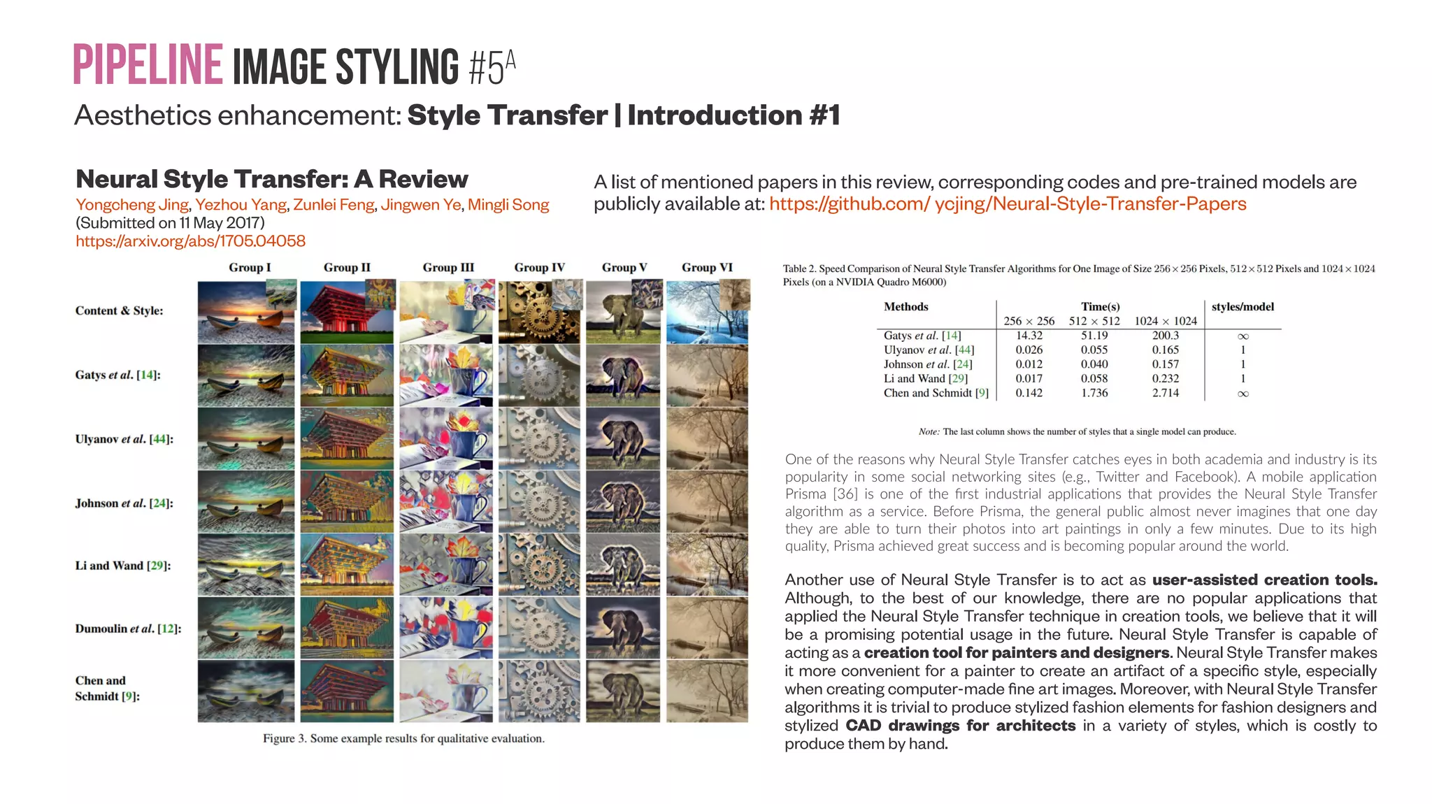
![Pipelineimage Styling #5A Aesthetics enhancement: Style Transfer | Introduction #1 Neural Style Transfer: A Review Yongcheng Jing, Yezhou Yang, Zunlei Feng, Jingwen Ye, Mingli Song (Submitted on 11 May 2017) https://arxiv.org/abs/1705.04058 A list of mentioned papers in this review, corresponding codes and pre-trained models are publicly available at: https://github.com/ ycjing/Neural-Style-Transfer-Papers One of the reasons why Neural Style Transfer catches eyes in both academia and industry is its popularity in some social networking sites (e.g., Twitter and Facebook). A mobile application Prisma [36] is one of the first industrial applications that provides the Neural Style Transfer algorithm as a service. Before Prisma, the general public almost never imagines that one day they are able to turn their photos into art paintings in only a few minutes. Due to its high quality, Prisma achieved great success and is becoming popular around the world. Another use of Neural Style Transfer is to act as user-assisted creation tools. Although, to the best of our knowledge, there are no popular applications that applied the Neural Style Transfer technique in creation tools, we believe that it will be a promising potential usage in the future. Neural Style Transfer is capable of acting as a creation tool for painters and designers. Neural Style Transfer makes it more convenient for a painter to create an artifact of a specific style, especially when creating computer-made fine art images. Moreover, with Neural Style Transfer algorithms it is trivial to produce stylized fashion elements for fashion designers and stylized CAD drawings for architects in a variety of styles, which is costly to produce them by hand.](https://image.slidesharecdn.com/datasetmultiviewcreation-170822074203/75/Dataset-creation-for-Deep-Learning-based-Geometric-Computer-Vision-problems-46-2048.jpg)
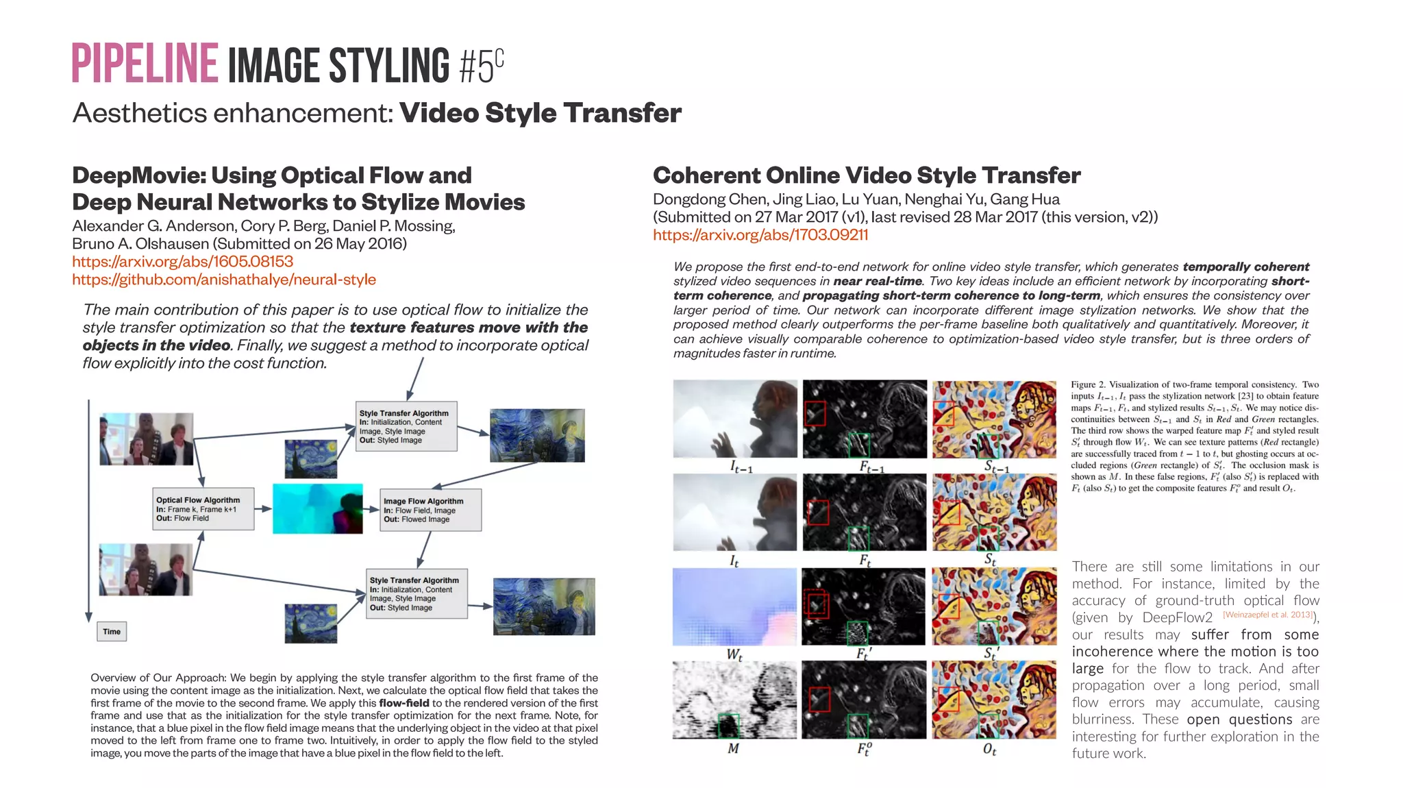
![Pipelineimage Styling #5C Aesthetics enhancement: Video Style Transfer DeepMovie: Using Optical Flow and Deep Neural Networks to Stylize Movies Alexander G. Anderson, Cory P. Berg, Daniel P. Mossing, Bruno A. Olshausen (Submitted on 26 May 2016) https://arxiv.org/abs/1605.08153 https://github.com/anishathalye/neural-style Coherent Online Video Style Transfer Dongdong Chen, Jing Liao, Lu Yuan, Nenghai Yu, Gang Hua (Submitted on 27 Mar 2017 (v1), last revised 28 Mar 2017 (this version, v2)) https://arxiv.org/abs/1703.09211 The main contribution of this paper is to use optical flow to initialize the style transfer optimization so that the texture features move with the objects in the video. Finally, we suggest a method to incorporate optical flow explicitly into the cost function. Overview of Our Approach: We begin by applying the style transfer algorithm to the first frame of the movie using the content image as the initialization. Next, we calculate the optical flow field that takes the first frame of the movie to the second frame. We apply this flow-field to the rendered version of the first frame and use that as the initialization for the style transfer optimization for the next frame. Note, for instance, that a blue pixel in the flow field image means that the underlying object in the video at that pixel moved to the left from frame one to frame two. Intuitively, in order to apply the flow field to the styled image, you move the parts of the image that have a blue pixel in the flow field to the left. We propose the first end-to-end network for online video style transfer, which generates temporally coherent stylized video sequences in near real-time. Two key ideas include an efficient network by incorporating short- term coherence, and propagating short-term coherence to long-term, which ensures the consistency over larger period of time. Our network can incorporate different image stylization networks. We show that the proposed method clearly outperforms the per-frame baseline both qualitatively and quantitatively. Moreover, it can achieve visually comparable coherence to optimization-based video style transfer, but is three orders of magnitudes faster in runtime. There are still some limitations in our method. For instance, limited by the accuracy of ground-truth optical flow (given by DeepFlow2 [Weinzaepfel et al. 2013] ), our results may suffer from some incoherence where the motion is too large for the flow to track. And after propagation over a long period, small flow errors may accumulate, causing blurriness. These open questions are interesting for further exploration in the future work.](https://image.slidesharecdn.com/datasetmultiviewcreation-170822074203/75/Dataset-creation-for-Deep-Learning-based-Geometric-Computer-Vision-problems-48-2048.jpg)
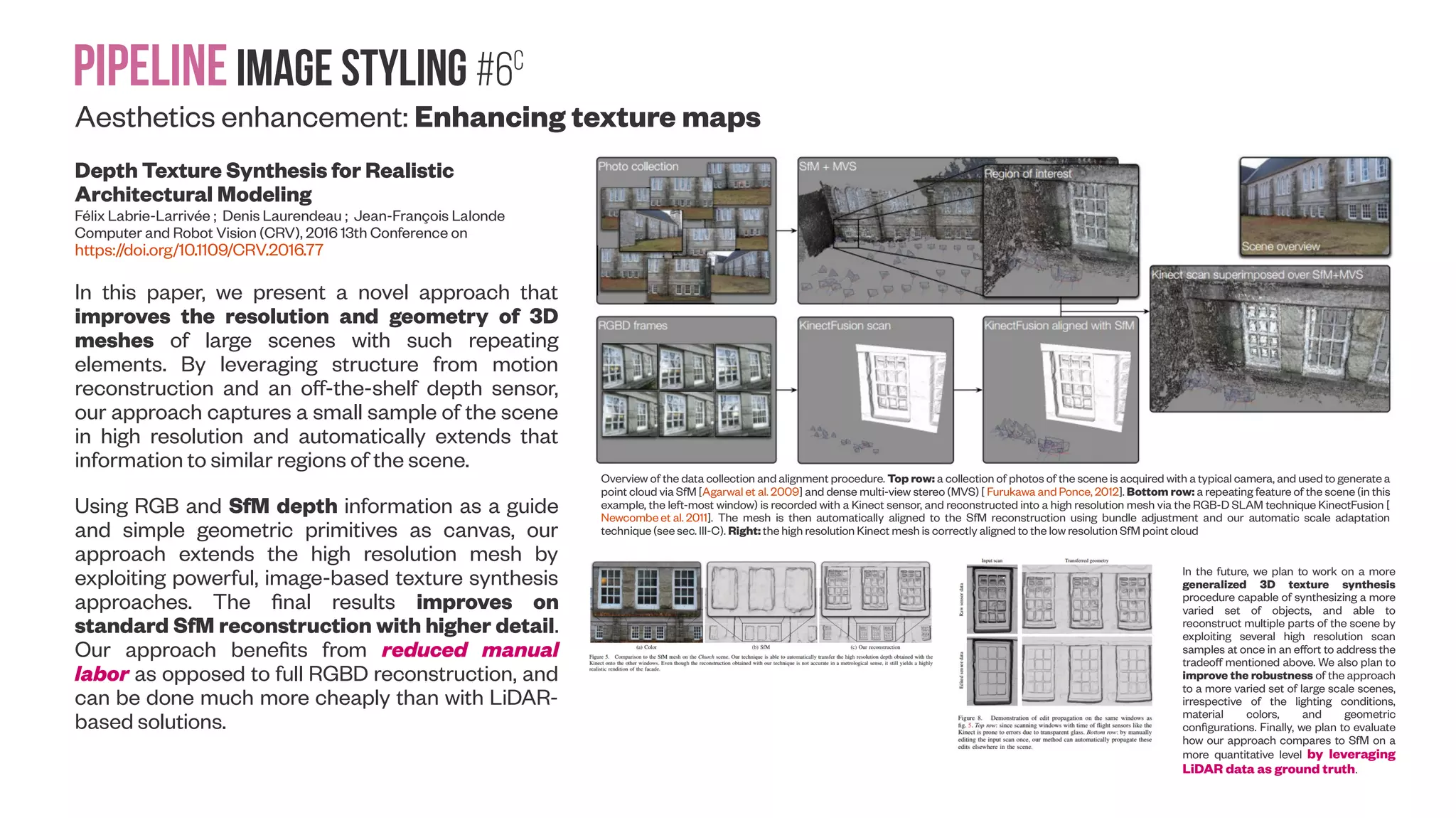
![Pipelineimage Styling #6C Aesthetics enhancement: Enhancing texture maps Depth Texture Synthesis for Realistic Architectural Modeling Félix Labrie-Larrivée ; Denis Laurendeau ; Jean-François Lalonde Computer and Robot Vision (CRV), 2016 13th Conference on https://doi.org/10.1109/CRV.2016.77 In this paper, we present a novel approach that improves the resolution and geometry of 3D meshes of large scenes with such repeating elements. By leveraging structure from motion reconstruction and an off-the-shelf depth sensor, our approach captures a small sample of the scene in high resolution and automatically extends that information to similar regions of the scene. Using RGB and SfM depth information as a guide and simple geometric primitives as canvas, our approach extends the high resolution mesh by exploiting powerful, image-based texture synthesis approaches. The final results improves on standard SfM reconstruction with higher detail. Our approach benefits from reduced manual labor as opposed to full RGBD reconstruction, and can be done much more cheaply than with LiDAR- based solutions. In the future, we plan to work on a more generalized 3D texture synthesis procedure capable of synthesizing a more varied set of objects, and able to reconstruct multiple parts of the scene by exploiting several high resolution scan samples at once in an effort to address the tradeoff mentioned above. We also plan to improve the robustness of the approach to a more varied set of large scale scenes, irrespective of the lighting conditions, material colors, and geometric configurations. Finally, we plan to evaluate how our approach compares to SfM on a more quantitative level by leveraging LiDAR data as ground truth. Overview of the data collection and alignment procedure. Top row: a collection of photos of the scene is acquired with a typical camera, and used to generate a point cloud via SfM [Agarwal et al. 2009] and dense multi-view stereo (MVS) [ Furukawa and Ponce, 2012]. Bottom row: a repeating feature of the scene (in this example, the left-most window) is recorded with a Kinect sensor, and reconstructed into a high resolution mesh via the RGB-D SLAM technique KinectFusion [ Newcombe et al. 2011]. The mesh is then automatically aligned to the SfM reconstruction using bundle adjustment and our automatic scale adaptation technique (see sec. III-C). Right: the high resolution Kinect mesh is correctly aligned to the low resolution SfM point cloud](https://image.slidesharecdn.com/datasetmultiviewcreation-170822074203/75/Dataset-creation-for-Deep-Learning-based-Geometric-Computer-Vision-problems-51-2048.jpg)
![PipelineDepth image enhancement #1a Image Formation #1 Pinhole Camera Model: ideal projection of a 3D object on a 2D image. Fernandez et al. (2017) Dot patterns of a Kinect for Windows (a) and two Kinects for Xbox (b) and (c) are projected on a flat wall from a distance of 1000 mm. Note that the projection of each pattern is similar, and related by a 3-D rotation depending on the orientation of the Kinect diffuser installation. The installation variability can clearly be observed from differences in the bright dot locations (yellow stars), which differ by an average distance of 10 pixels. Also displayed in (d) is the idealized binary replication of the Kinect dot pattern [Kinect Patter Uncovered] , which was used in this project to simulate IR images. - Landau et al. (2016) Landau et al. (2016)](https://image.slidesharecdn.com/datasetmultiviewcreation-170822074203/75/Dataset-creation-for-Deep-Learning-based-Geometric-Computer-Vision-problems-55-2048.jpg)
![PipelineDepth image enhancement #1b Image Formation #2 Characterizations of Noise in Kinect Depth Images: A Review Tanwi Mallick ; Partha Pratim Das ; Arun Kumar Majumdar IEEE Sensors Journal ( Volume: 14, Issue: 6, June 2014 ) https://doi.org/10.1109/JSEN.2014.2309987 Kinect outputs for a scene. (a) RGB Image. (b) Depth data rendered as an 8- bit gray-scale image with nearer depth values mapped to lower intensities. Invalid depth values are set to 0. Note the fixed band of invalid (black) pixels on left. (c) Depth image showing too near depths in blue, too far depths in red and unknown depths due to highly specular objects in green. Often these are all taken as invalid zero depth. Shadow is created in a depth image (Yu et al. 2013) when the incident IR from the emitter gets obstructed by an object and no depth can be estimated. PROPERTIES OF IR LIGHT [Rose]](https://image.slidesharecdn.com/datasetmultiviewcreation-170822074203/75/Dataset-creation-for-Deep-Learning-based-Geometric-Computer-Vision-problems-56-2048.jpg)
![Pipeline Depth image enhancement #1c Image Formation #3 Authors’ experiments on structural noise using a plane in 400 frames. (a) Error at 1.2m. (b) Error at 1.6m. (c) Error at 1.8m. Smisek et al. (2013) calibrate a Kinect against a stereo-rig (comprising two Nikon D60 DSLR cameras) to estimate and improve its overall accuracy. They have taken images and fitted planar objects at 18 different distances (from 0.7 to 1.3 meters) to estimate the error between the depths measured by the two sensors. The experiments corroborate that the accuracy varies inversely with the square of depth [2]. However, even after the calibration of Kinect, the procedure still exhibits relatively complex residual errors (Fig. 8). Fig. 8. Residual noise of a plane. (a) Plane at 86cm. (b) Plane at 104cm. Authors’ experiments on temporal noise. Entropy and SD of each pixel in a depth frame over 400 frames for a stationary wall at 1.6m. (a) Entropy image. (b) SD image. Authors’ experiments with vibrating noise showing ZD samples as white dots. A pixel is taken as noise if it is zero in frame i and nonzero in frames i±1. Note that noise follows depth edges and shadow. (a) Frame (i−1). (b) Frame i. (c) Frame (i+1). (d) Noise for frame i.](https://image.slidesharecdn.com/datasetmultiviewcreation-170822074203/75/Dataset-creation-for-Deep-Learning-based-Geometric-Computer-Vision-problems-57-2048.jpg)

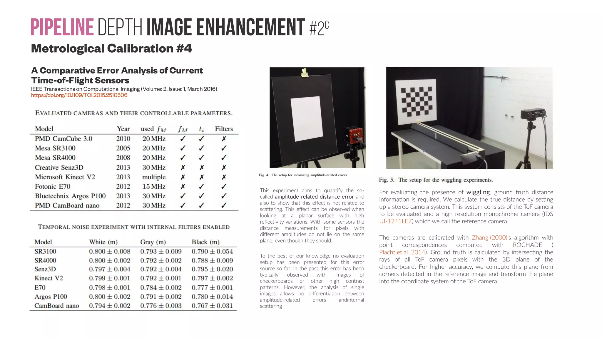
![PipelineDepth image enhancement #2A Metrological Calibration #1 A New Calibration Method for Commercial RGB-D Sensors Walid Darwish, Shenjun Tang, Wenbin Li and Wu Chen Sensors 2017, 17(6), 1204; doi:10.3390/s17061204 Based on these calibration algorithms, different calibration methods have been implemented and tested. Methods include the use of 1D [Liu et al. 2012] 2D [Shibo and Qing 2012] , and 3D [Gui et al. 2014] calibration objects that work with the depth images directly; calibration of the manufacture parameters of the IR camera and projector [Herrera et al. 2012] ; or photogrammetric bundle adjustments used to model the systematic errors of the IR sensors [ Davoodianidaliki and Saadatseresht 2013; Chow and Lichti 2013] . To enhance the depth precision, additional depth error models are added to the calibration procedure [7,8,21,22,23]. All of these error models are used to compensate only for the distortion effect of the IR projector and camera. Other research works have been conducted to obtain the relative calibration between an RGB camera and an IR camera by accessing the IR camera [24,25,26]. This can achieve relatively high accuracy calibration parameters for a baseline between IR and RGB cameras, while the remaining limitation is that the distortion parameters for the IR camera cannot represent the full distortion effect for the depth sensor. This study addressed these issues using a two-step calibration procedure to calibrate all of the geometric parameters of RGB-D sensors. The first step was related to the joint calibration between the RGB and IR cameras, which was achieved by adopting the procedure discussed in [27] to compute the external baseline between the cameras and the distortion parameters of the RGB camera. The second step focused on the depth sensor calibration. Point cloud of two perpendicular planes (blue color: default depth; red color: modeled depth): highlighted black dashed circles shows the significant impact of the calibration method on the point cloud quality. The main difference between both sensors is the baseline between the IR camera and projector. The longer the sensor’s baseline, the longer working distance can be achieved. The working range of Kinect v1 is 0.80 m to 4.0 m, while it is 0.35 m to 3.5 m for Structure Sensor.](https://image.slidesharecdn.com/datasetmultiviewcreation-170822074203/75/Dataset-creation-for-Deep-Learning-based-Geometric-Computer-Vision-problems-59-2048.jpg)
![PipelineDepth image enhancement #3 ‘Old-school’ depth refining techniques Depth enhancement with improved exemplar-based inpainting and joint trilateral guided filtering Liang Zhang ; Peiyi Shen ; Shu'e Zhang ; Juan Song ; Guangming Zhu Image Processing (ICIP), 2016 IEEE International Conference on https://doi.org/10.1109/ICIP.2016.7533131 In this paper, a novel depth enhancement algorithm with improved exemplar-based inpainting and joint trilateral guided filtering is proposed. The improved examplar-based inpainting method is applied to fill the holes in the depth images, in which the level set distance component is introduced in the priority evaluation function. Then a joint trilateral guided filter is adopted to denoise and smooth the inpainted results. Experimental results reveal that the proposed algorithm can achieve better enhancement results compared with the existing methods in terms of subjective and objective quality measurements. Robust depth enhancement and optimization based on advanced multilateral filters Ting-An ChangYang-Ting ChouJar-Ferr Yang EURASIP Journal on Advances in Signal Processing December 2017, 2017:51 https://doi.org/10.1186/s13634-017-0487-7 Results of the depth enhancement coupled with hole filling results obtainedby a noisy depth map, b joint bilateral filter (JBF) [16 ], c intensity guided depth superresolution (IGDS) [39], d compressive sensing based depth upsampling (CSDU) [40], e adaptive joint trilateral filter (AJTF) [18], and f the proposed AMF for Art, Books, Doily, Moebius, RGBD_1, and RGBD_2](https://image.slidesharecdn.com/datasetmultiviewcreation-170822074203/75/Dataset-creation-for-Deep-Learning-based-Geometric-Computer-Vision-problems-64-2048.jpg)
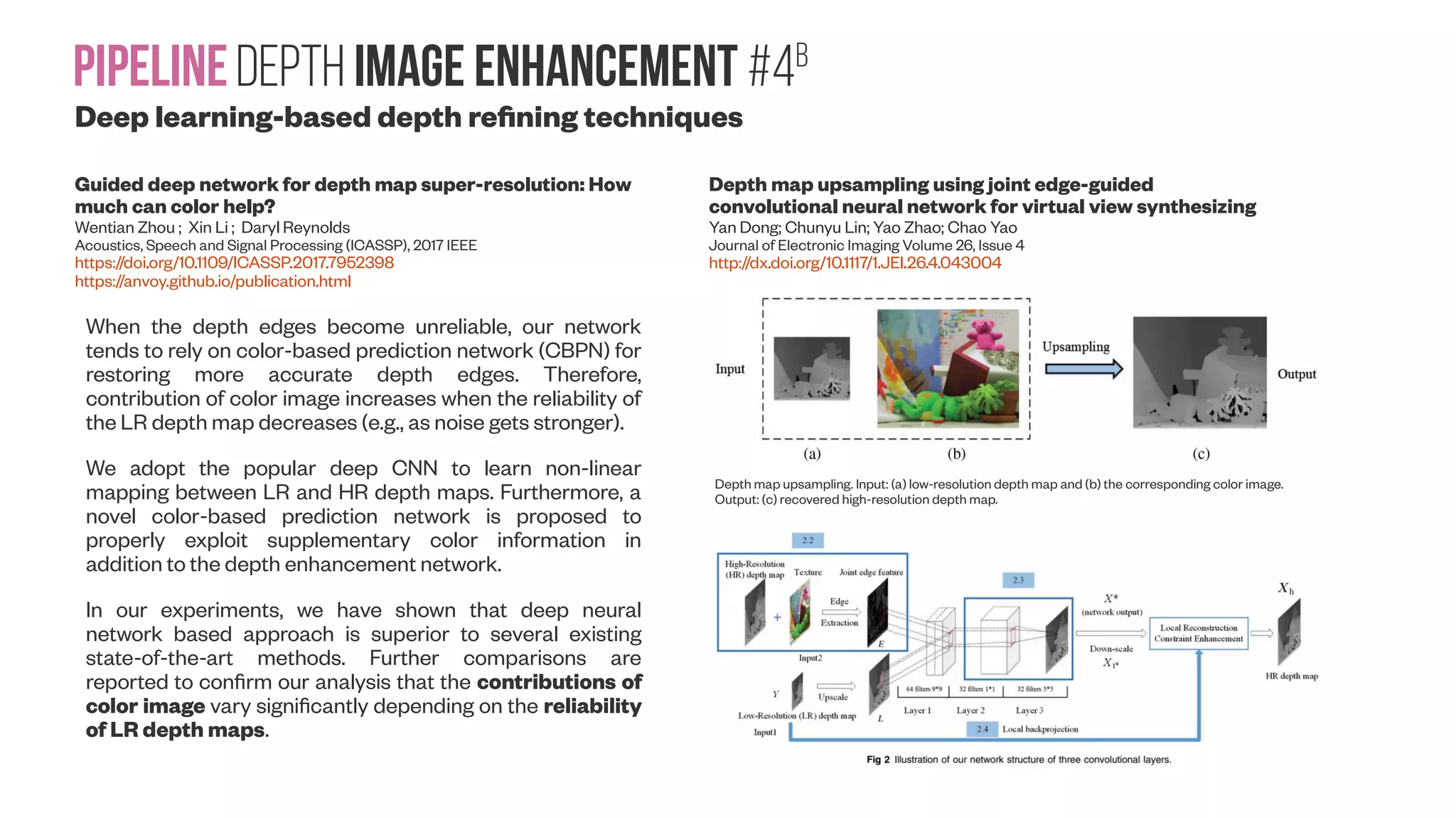
![PipelineDepth image enhancement #4A Deep learning-based depth refining techniques DepthComp : real-time depth image completion based on prior semantic scene segmentation Atapour-Abarghouei, A. and Breckon, T.P. 28th British Machine Vision Conference (BMVC) 2017 London, UK, 4-7 September 2017. http://dro.dur.ac.uk/22375/ Exemplar results on the KITTI dataset. S denotes the segmented images [3] and D the original (unfilled) disparity maps. Results are compared with [1, 2, 29, 35, 45]. Results of cubic and linear interpolations are omitted due to space. Comparison of the proposed method using different initial segmentation techniques on the KITTI dataset [27]. Original color and disparity image (top-left), results with manual labels (top-right), results with SegNet [3] (bottom-left) and results with mean-shift [26] (bottom-right). Fast depth image denoising and enhancement using a deep convolutional network Xin Zhang and Ruiyuan Wu Acoustics, Speech and Signal Processing (ICASSP), 2016 IEE https://doi.org/10.1109/ICASSP.2016.7472127](https://image.slidesharecdn.com/datasetmultiviewcreation-170822074203/75/Dataset-creation-for-Deep-Learning-based-Geometric-Computer-Vision-problems-65-2048.jpg)
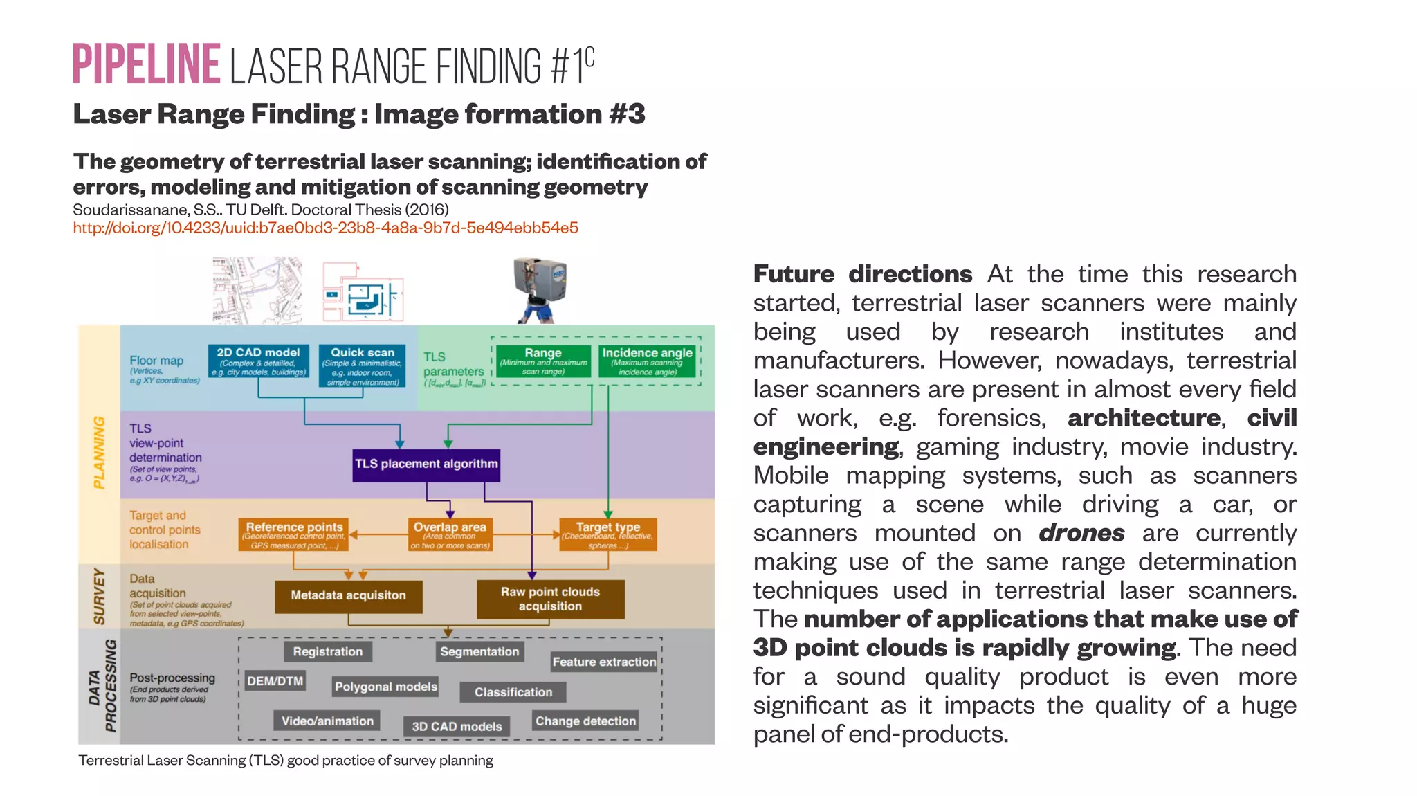
![PipelineLaser range Finding #1a Versatile Approach to Probabilistic Modeling of Hokuyo UTM-30LX IEEE Sensors Journal ( Volume: 16, Issue: 6, March15, 2016 ) https://doi.org/10.1109/JSEN.2015.2506403 When working with Laser Range Finding (LRF), it is necessary to know the principle of sensor’s measurement and its properties. There are several measurement principles used in LRFs [Nejad and Olyaee 2006], [ Łabęcki et al. 2012], [Adams 1999] : ● Triangulation ● Time of flight (TOF) ● Frequency modulation continuous wave (FMCW) ● Phase shift measurement (PSM) The geometry of terrestrial laser scanning; identification of errors, modeling and mitigation of scanning geometry Soudarissanane, S.S.. TU Delft. Doctoral Thesis (2016) http://doi.org/10.4233/uuid:b7ae0bd3-23b8-4a8a-9b7d-5e494ebb54e5 Distance measurement principle of time-of-flight laser scanners (top) and phase based laser scanners (bottom). Laser Range Finding : Image formation #1](https://image.slidesharecdn.com/datasetmultiviewcreation-170822074203/75/Dataset-creation-for-Deep-Learning-based-Geometric-Computer-Vision-problems-68-2048.jpg)
![PipelineLaser range Finding #1b Laser Range Finding : Image formation #2 The geometry of terrestrial laser scanning; identification of errors, modeling and mitigation of scanning geometry Soudarissanane, S.S.. TU Delft. Doctoral Thesis (2016) http://doi.org/10.4233/uuid:b7ae0bd3-23b8-4a8a-9b7d-5e494ebb54e5 Two ways link budget between the receiver (Rx) and the transmitter (Tx) in a Free Space Path (FSP) propagation model. Schematic representation of the signal propagation from the transmitter to the receiver. Effect of increasing incidence angle and range to the signal deterioration. (left) Plot of the the signal deterioration due to increasing incidence angle α, (right) plot of the signal deterioration due to increasing ranges ρ, with ρmin = 0 m and ρmax = 100 m Relationship between scan angle and normal vector orientation used for the segmentation of point cloud with respect to planar features. A point P = [ , , ]θ ϕ ρ is measured on the plane with the normal parameters N = [ , , ]α β γ . Different angles used for the range image gradients are plotted Theoretical number of points. Practical example of a plate of 1×1 m placed at 3 m, oriented at 0º and being rotated at 60º. Theoretical number of points. (left) Number of points with respect to the orientation of the patch and the distance. Reference plate measurement set-up. A white coated plywood board is mounted on a tripod via a screw clamp mechanism provided with a 2º precision goniometer.](https://image.slidesharecdn.com/datasetmultiviewcreation-170822074203/75/Dataset-creation-for-Deep-Learning-based-Geometric-Computer-Vision-problems-69-2048.jpg)
![PipelineLaser range Finding #2c Calibration #3 Towards System Calibration of Panoramic Laser Scanners from a Single Station Tomislav Medić, Christoph Holst and Heiner Kuhlmann Sensors 2017, 17(5), 1145; doi: 10.3390/s17051145 “Terrestrial laser scanner measurements suffer from systematic errors due to internal misalignments. The magnitude of the resulting errors in the point cloud in many cases exceeds the magnitude of random errors. Hence, the task of calibrating a laser scanner is important for applications with high accuracy demands. In order to achieve the required measurement quality, manufacturers put considerable effort on the production and assembly of all instrument components. However, these processes are not perfect and remaining mechanical misalignments need to be modeled mathematically. That is achieved by a comprehensive factory calibration (e.g., [4]). In general, manufacturers do not provide complete information about the functional relations between the remaining mechanical misalignments and the observations, the number of relevant misalignments, as well as the magnitude and precision of the parameters describing those misalignments. This data is treated as a company secret. At the time of purchase, laser scanners are expected to be free of systematic errors caused by mechanical misalignments. Additionally, their measurement quality should be consistent with the description given in the manufacturers specifications. However, many factors can influence the performance of the particular scanner, such as long-term utilization, suffered stresses and extreme atmospheric conditions. Due to that, instruments must be tested and recalibrated at certain time intervals in order to maintain the declared measurement quality. There are certain alternatives, but they lack in comprehensiveness and reliability. For example, some manufacturers like Leica Geosystems and FARO Inc. provide user calibration approaches, which can reduce systematic errors in the measurements due to misalignments to some extent (e.g., Leica’s “Check and Adjust” and Faro’s “On-site compensation”). However, those approaches do not provide detailed information about all estimated parameters, their precision and influence on the resulting point cloud. Perfect panoramic terrestriallaser scanner geometry. (a) Local Cartesian coordinate system of the scanner with a respect to the main instrument axes; (b) Local coordinate system of the scanner transformed to the polar coordinates. Rotational mirror related mechanical misalignments: (a) mirror offset; (b) mirror tilt. Horizontal axis related mechanical misalignments: (a) axis offset; (b) axis tilt.](https://image.slidesharecdn.com/datasetmultiviewcreation-170822074203/75/Dataset-creation-for-Deep-Learning-based-Geometric-Computer-Vision-problems-74-2048.jpg)
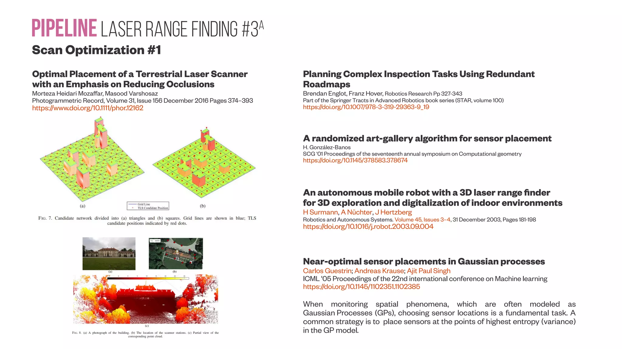
![PipelineLaser range Finding #3C Scan Optimization #3 Active Image-based Modeling Rui Huang, Danping Zou, Richard Vaughan, Ping Tan (Submitted on 2 May 2017) https://arxiv.org/abs/1705.01010 Plan3D: Viewpoint and Trajectory Optimization for Aerial Multi-View Stereo Reconstruction Benjamin Hepp, Matthias Nießner, Otmar Hilliges (Submitted on 25 May 2017) https://arxiv.org/abs/1705.09314 We propose an end-to-end system for 3D reconstruction of building-scale scenes with commercially available quadrotors. (A) A user defines the region of interest (green) on a map-based interface and specifies a pattern of viewpoints (orange), flown at a safe altitude. (B) The pattern is traversed and the captured images are processed resulting in an initial reconstruction and occupancy map. (C) We compute a viewpoint path that observes as much of the unknown space as possible adhering to characteristics of a purposeful designed camera model. The viewpoint path is only allowed to pass through known free space and thus the trajectory can be executed fully autonomously. (D) The newly captured images are processed together with the initial images to attain the final high-quality reconstruction of the region of interest. The method is capable of capturing concave areas and fine geometric detail. Comparison several iterations of our method for the church scene. Note that some prominent structures get only resolved in the second iteration. Also the overall sharpness of the walls and ornaments significantly improves with the second iteration. Modeling of an Asian building after the initial data capturing (a) and actively capturing more data (b). The figures (a.1), (b.1) show the SfM point clouds and camera poses, (a.2), (b.2) are color-coded model quality evaluation, where red indicates poor results, (a.3), (b.3) are the final 3D models generated from those images. Our system consists of an online front end and an offline back end. The front end captures images automatically to ensure good coverage of the object. The back end takes an existing method [Jancosek and Pajdla, 2011] to build a high quality 3D model.](https://image.slidesharecdn.com/datasetmultiviewcreation-170822074203/75/Dataset-creation-for-Deep-Learning-based-Geometric-Computer-Vision-problems-77-2048.jpg)
![PipelineLaser range Finding #4E Scan Optimization #5 A Reinforcement Learning Approach to the View Planning Problem Mustafa Devrim Kaba, Mustafa Gokhan Uzunbas, Ser Nam Lim Submitted on 19 Oct 2016, last revised 18 Nov 2016 https://arxiv.org/abs/1610.06204 (a) View planning for UAV terrain modeling, (b) Given a set of initial view points, (c) The goal is to find minimum number of views that provide sufficient coverage. Here, color code represents correspondence between selected views and the coverage. Visual results of coverage and sample views on various models. In the top row, lines represent location and direction of the selected cameras. Colors represent coverage by different cameras. Data Driven Strategies for Active Monocular SLAM using Inverse Reinforcement Learning Vignesh Prasad, Rishabh Jangir, Ravindran Balaraman, K. Madhava Krishna AAMAS '17 Proceedings of the 16th Conference on Autonomous Agents and MultiAgent Systems http://www.aamas2017.org/proceedings/pdfs/p1697.pdf Gazebo [Koenig and Howard, 2004] is a framework that accurately simulates robots and dynamic environments. Experiments were performed in simulated environments on a Turtlebot using a Microsoft Kinect for the RGB camera input. We use PTAM (Parallel Tracking and Mapping) [Klein and Murray, 2007] for the Monocular SLAM framework.](https://image.slidesharecdn.com/datasetmultiviewcreation-170822074203/75/Dataset-creation-for-Deep-Learning-based-Geometric-Computer-Vision-problems-79-2048.jpg)
![PipelineLaser range Finding SUMMARY Previous slides highlight the need to keep your scanner calibrated as proper calibration reduces standard deviation for depth measurement. If you are not familiar with optics metrology, for example in LEDs, the increased temperature (T) will decrease light intensity even with constant forward current (If ) and shift peak wavelength (λ). Exact effects then depend on the laser type, and reading the datasheet might be helpful if available for your laser scanner And the light sensor (photodiode) has a wavelength and temperature-dependent sensitivity response: For deep learning purposes, lack of calibration of mid-quality targets (not the highest quality gold standard) could be used for “physics-true” data augmentation in addition to synthetic data augmentation Prof E. Fred Schubert "Light-Emitting Diodes" Second Edition (ISBN-13: 978-0-9863826-1-1) https://www.ecse.rpi.edu/~schubert/Ligh t-Emitting-Diodes-dot-org/chap06/chap06 .htm Ma et al. (2015) Spectral response characteristics of various IR detectors of different materials/technologies. Detectivity (vertical axis) is a measure of signal-to-noise ratio (SNR) of an imager normalized for its pixel area and noise bandwidth [Hamamatsu]. Sood et al. (2015) Room temperature emission spectra under He-Cd 325 nm laser excitation of ZnO:Pr (0.9%) fi lms prepared at di ff erent deposition temperatures and after annealing. The inset provides a closer picture of the main Pr 3+ emission peak, without the contribution Balestrieri et al. (2014)](https://image.slidesharecdn.com/datasetmultiviewcreation-170822074203/75/Dataset-creation-for-Deep-Learning-based-Geometric-Computer-Vision-problems-80-2048.jpg)
![Pipeline Commercial Laser Scanners Low-cost LiDARs #1 A low-cost laser distance sensor Kurt Konolige ; Joseph Augenbraun ; Nick Donaldson ; Charles Fiebig ; Pankaj Shah Robotics and Automation, 2008. ICRA 2008. IEEE https://doi.org/10.1109/ROBOT.2008.4543666 Revo LDS. Approximate width is 10cm. Round carrier spins, holds optical module with laser dot module, imager, and lens. The Electrolux Trilobite, one of the only cleaners to make a map, relies on sonar sensors [Zunino and Christensen, 2002]. The barrier to using laser distance sensor (LDS) technology is the cost. The two most common devices, the SICK LMS 200 [ Alwan et al. 2005] and the Hokuyo URG- 04LX [Alwan et al. 2005], cost an order of magnitude more than the simplest robot In this paper we describe a compact, low-cost (~$30 cost to build) LDS that is as capable as standard LDS devices, yet is being manufactured for a fraction of their cost: the Revo LDS. Comparing low-cost 2D scanning Lidars May 28, 2017 https://diyrobocars.com/2017/05/28/comparing-low-cost-2d-scanning-lidars/ The RP Lidar A2 (left) and the Scanse Sweep (right). The RP Lidar A2 is the second lidar from Slamtec, a Chinese company with a good track record. Sweep is the first lidar from Scanse, a US company https://youtu.be/yLPM2BVQ2Ws](https://image.slidesharecdn.com/datasetmultiviewcreation-170822074203/75/Dataset-creation-for-Deep-Learning-based-Geometric-Computer-Vision-problems-82-2048.jpg)
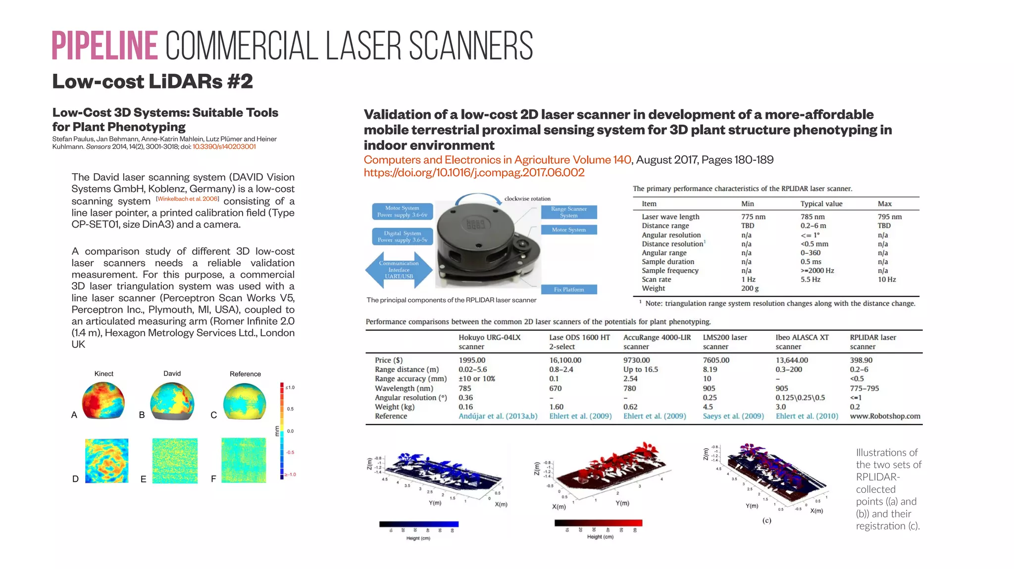
![Pipeline Commercial Laser Scanners Low-cost LiDARs #2 Low-Cost 3D Systems: Suitable Tools for Plant Phenotyping Stefan Paulus, Jan Behmann, Anne-Katrin Mahlein, Lutz Plümer and Heiner Kuhlmann. Sensors 2014, 14(2), 3001-3018; doi: 10.3390/s140203001 The David laser scanning system (DAVID Vision Systems GmbH, Koblenz, Germany) is a low-cost scanning system [Winkelbach et al. 2006] consisting of a line laser pointer, a printed calibration field (Type CP-SET01, size DinA3) and a camera. A comparison study of different 3D low-cost laser scanners needs a reliable validation measurement. For this purpose, a commercial 3D laser triangulation system was used with a line laser scanner (Perceptron Scan Works V5, Perceptron Inc., Plymouth, MI, USA), coupled to an articulated measuring arm (Romer Infinite 2.0 (1.4 m), Hexagon Metrology Services Ltd., London UK Validation of a low-cost 2D laser scanner in development of a more-affordable mobile terrestrial proximal sensing system for 3D plant structure phenotyping in indoor environment Computers and Electronics in Agriculture Volume 140, August 2017, Pages 180-189 https://doi.org/10.1016/j.compag.2017.06.002 The principal components of the RPLIDAR laser scanner Illustrations of the two sets of RPLIDAR- collected points ((a) and (b)) and their registration (c).](https://image.slidesharecdn.com/datasetmultiviewcreation-170822074203/75/Dataset-creation-for-Deep-Learning-based-Geometric-Computer-Vision-problems-83-2048.jpg)
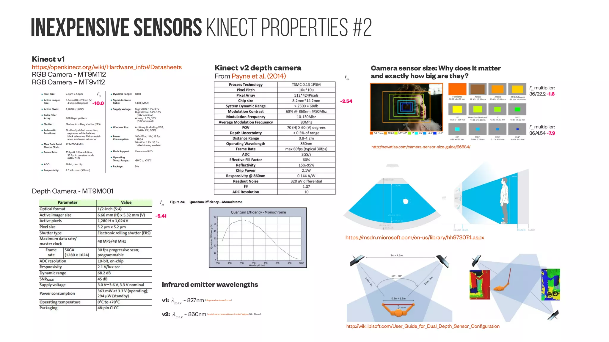
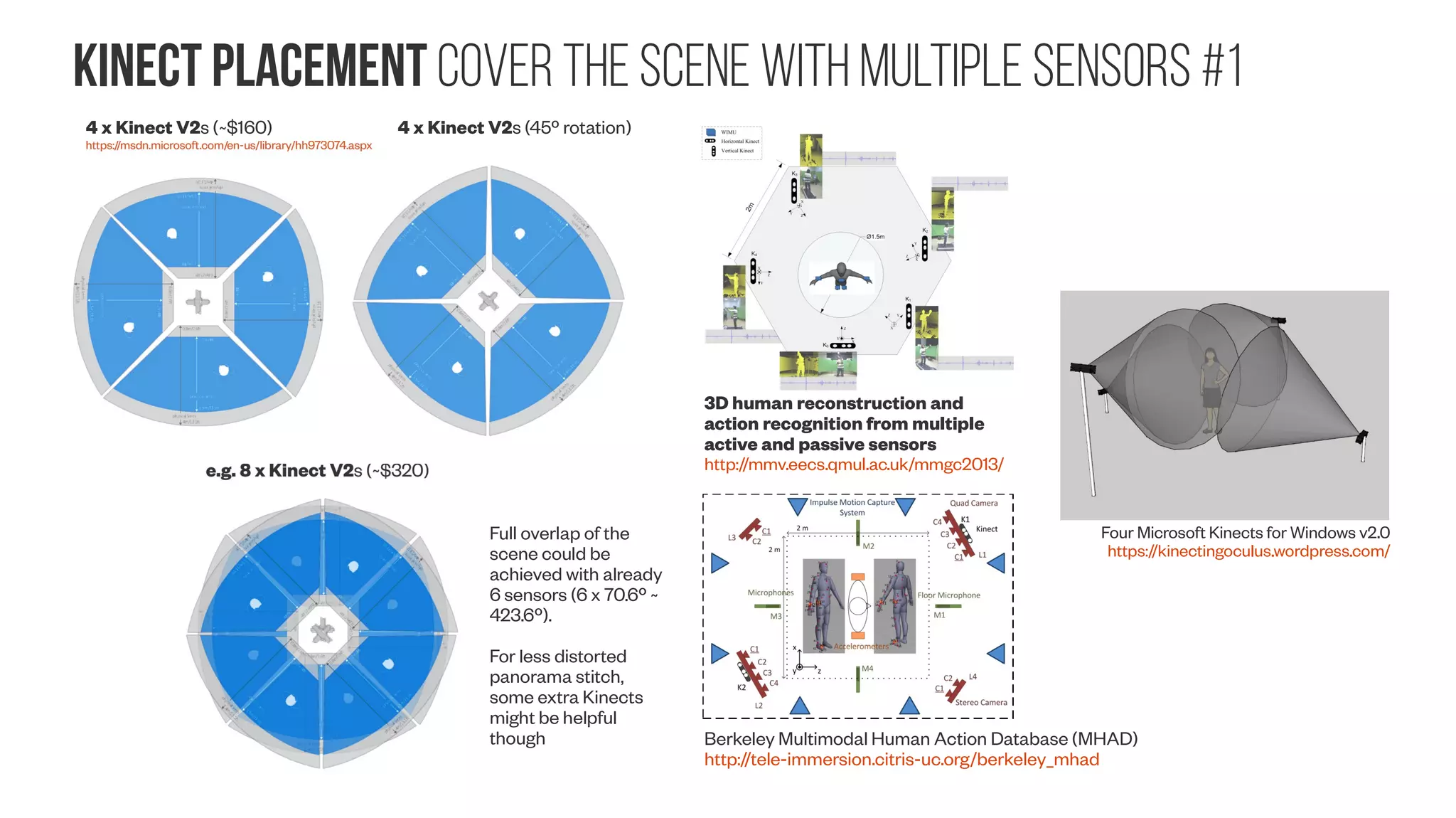
![inexpensive sensors Kinect properties #2 Kinect v1 https://openkinect.org/wiki/Hardware_info#Datasheets RGB Camera - MT9M112 RGB Camera – MT9v112 Depth Camera - MT9M001 Infrared emitter wavelengths v1: λmax ~ 827nm [blogs.msdn.microsoft.com] v2: λmax ~ 860nm [social.msdn.microsoft.com, Lembit Valgma BSc. Thesis] Kinect v2 depth camera From Payne et al. (2014) Camera sensor size: Why does it matter and exactly how big are they? http://newatlas.com/camera-sensor-size-guide/26684/ fm multiplier: 36/22.2 ~1.6 fm multiplier: 36/4.54 ~7.9 fm ~2.54 fm ~5.41 ~10.0 fm https://msdn.microsoft.com/en-us/library/hh973074.aspx http://wiki.ipisoft.com/User_Guide_for_Dual_Depth_Sensor_Configuration](https://image.slidesharecdn.com/datasetmultiviewcreation-170822074203/75/Dataset-creation-for-Deep-Learning-based-Geometric-Computer-Vision-problems-93-2048.jpg)


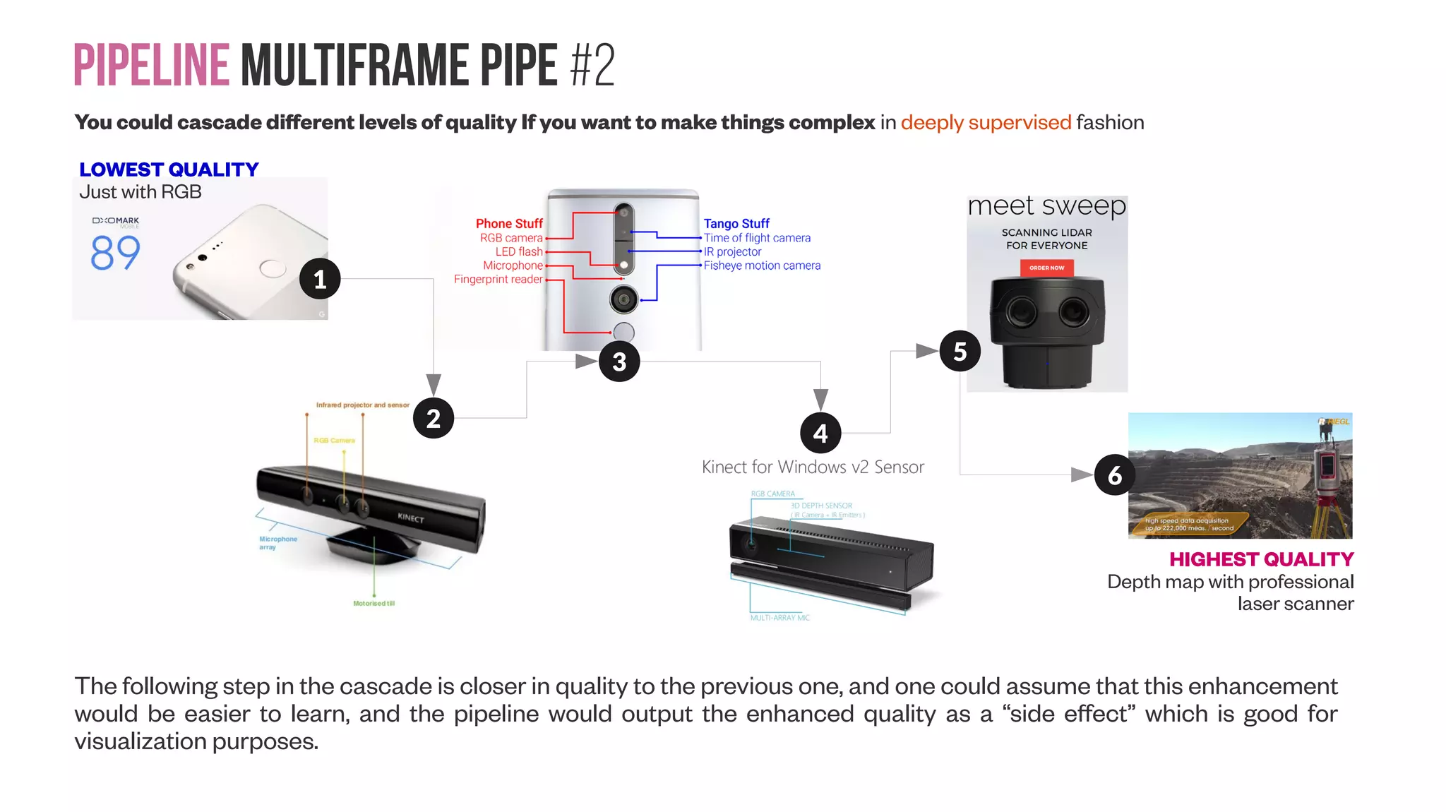
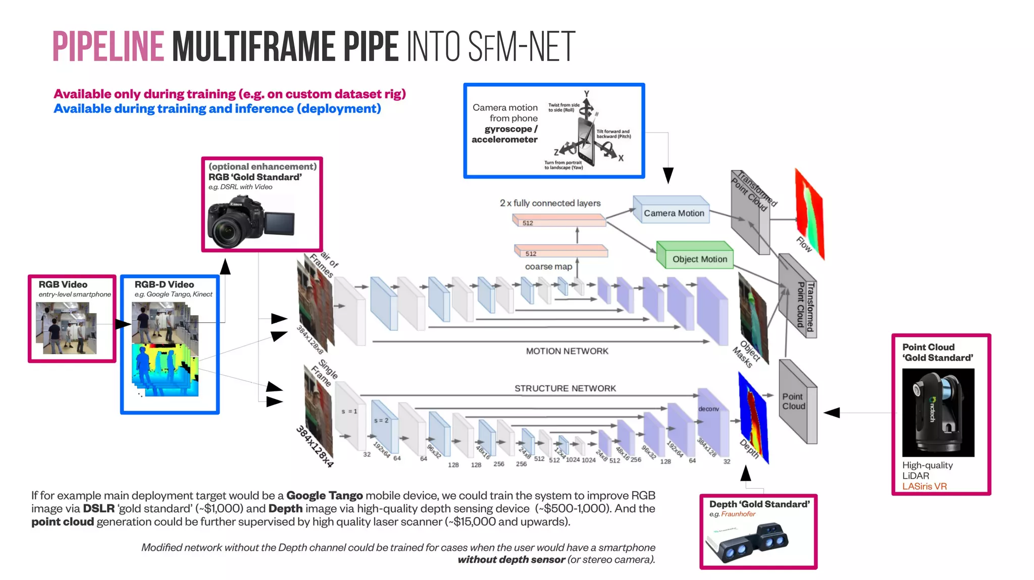
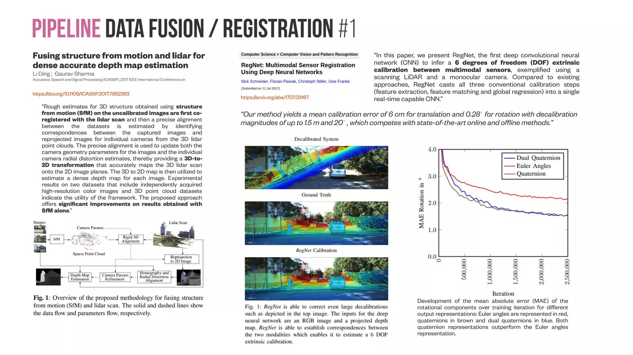
The document presents a comprehensive approach to creating datasets for deep learning in geometric computer vision, emphasizing the need for multi-sensor setups to obtain high-quality reference data. It discusses various pipeline configurations for dataset creation, including techniques for enhancing image resolution and depth accuracy through multiframe image processing. Additionally, it addresses challenges in sensor calibration, data fusion, and the importance of generating labeled data for effective training of deep learning models in robotic manipulation tasks.