Data structure Graph PPT ( BFS & DFS ) NOTES

Graphs: • Basic Concepts • Different representations of Graphs • Graph Traversals(BFS & DFS) • Minimum Spanning Tree (Prim & Kruskal algorithms) • Dijkstra’s shortest path algorithms • Hashing(Hash function, Address calculation techniques, Common Hashing functions) • Collision resolution: Linear and Quadratic probing • Double hashing

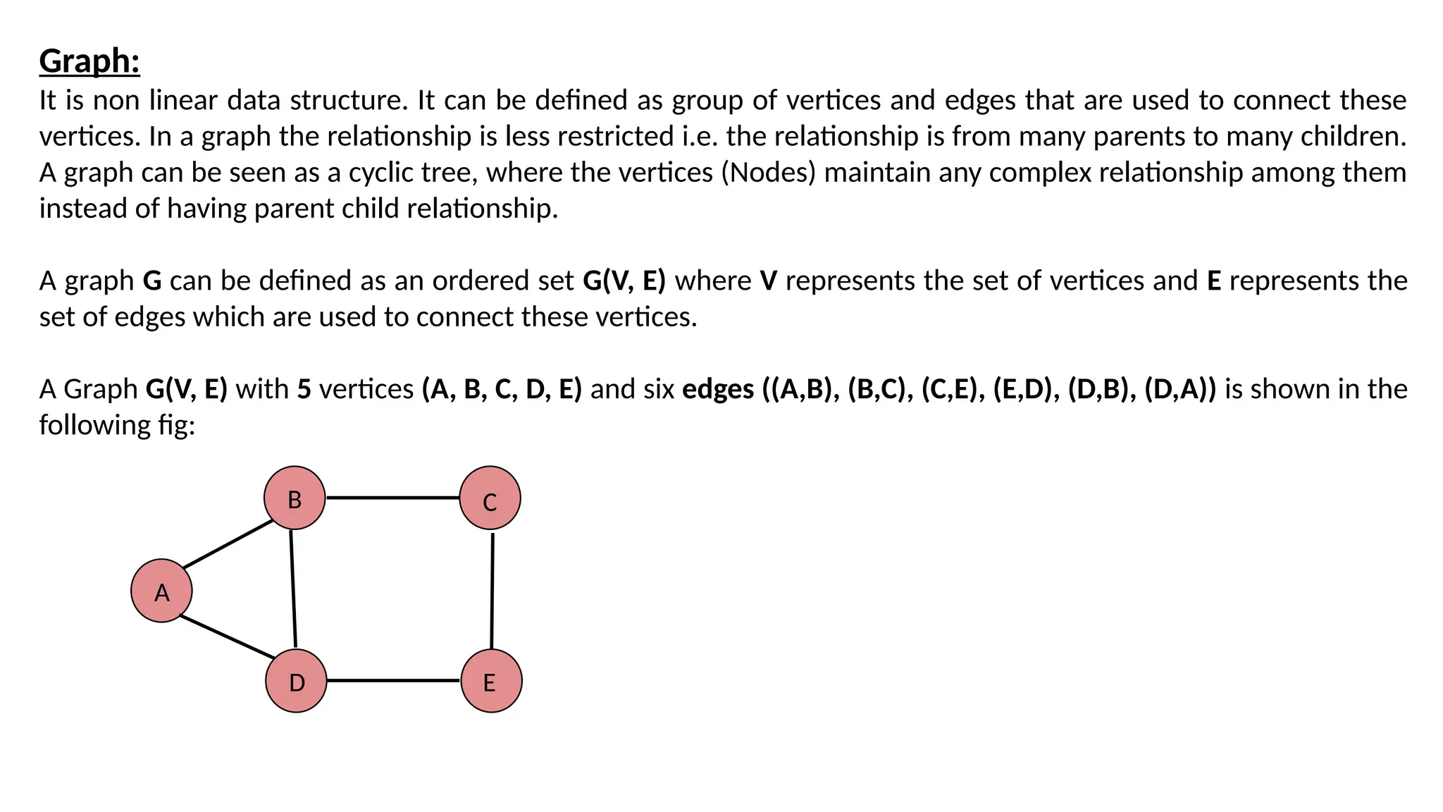
Graph: It is non linear data structure. It can be defined as group of vertices and edges that are used to connect these vertices. In a graph the relationship is less restricted i.e. the relationship is from many parents to many children. A graph can be seen as a cyclic tree, where the vertices (Nodes) maintain any complex relationship among them instead of having parent child relationship. A graph G can be defined as an ordered set G(V, E) where V represents the set of vertices and E represents the set of edges which are used to connect these vertices. A Graph G(V, E) with 5 vertices (A, B, C, D, E) and six edges ((A,B), (B,C), (C,E), (E,D), (D,B), (D,A)) is shown in the following fig: A B D C E

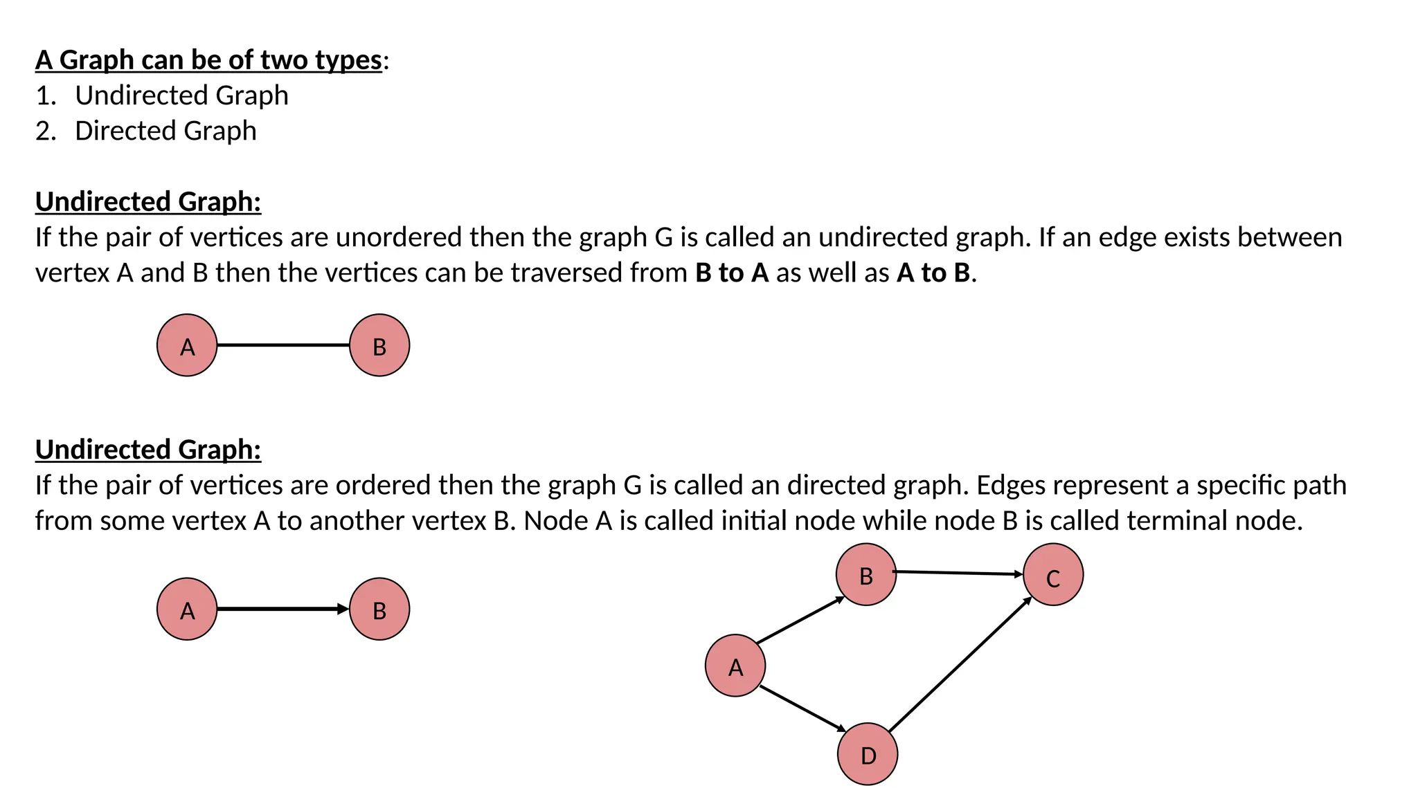
A Graph can be of two types: 1. Undirected Graph 2. Directed Graph Undirected Graph: If the pair of vertices are unordered then the graph G is called an undirected graph. If an edge exists between vertex A and B then the vertices can be traversed from B to A as well as A to B. Undirected Graph: If the pair of vertices are ordered then the graph G is called an directed graph. Edges represent a specific path from some vertex A to another vertex B. Node A is called initial node while node B is called terminal node. A B A B A B D C

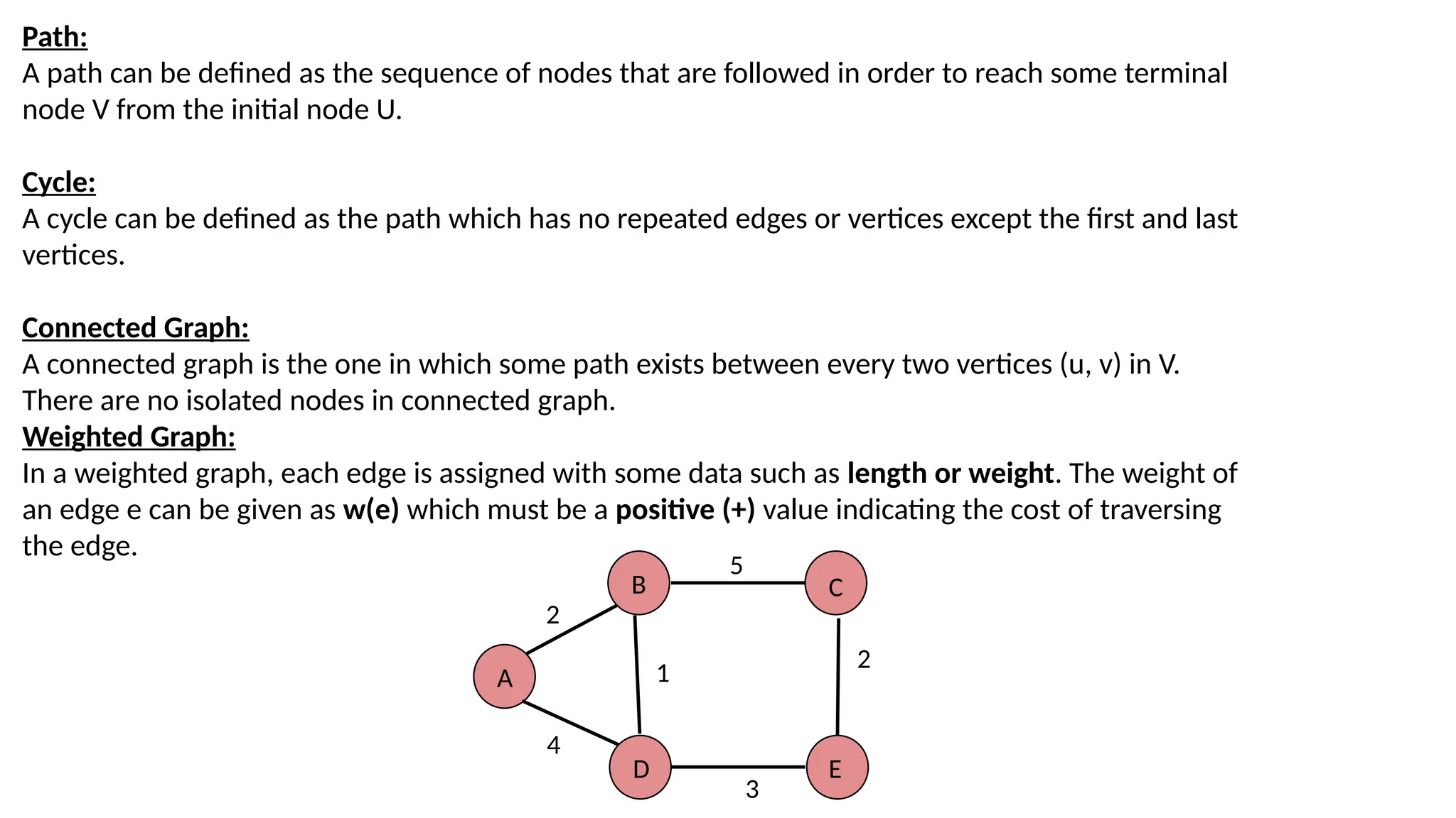
Path: A path can be defined as the sequence of nodes that are followed in order to reach some terminal node V from the initial node U. Cycle: A cycle can be defined as the path which has no repeated edges or vertices except the first and last vertices. Connected Graph: A connected graph is the one in which some path exists between every two vertices (u, v) in V. There are no isolated nodes in connected graph. Weighted Graph: In a weighted graph, each edge is assigned with some data such as length or weight. The weight of an edge e can be given as w(e) which must be a positive (+) value indicating the cost of traversing the edge. A B D C E 2 1 4 5 2 3

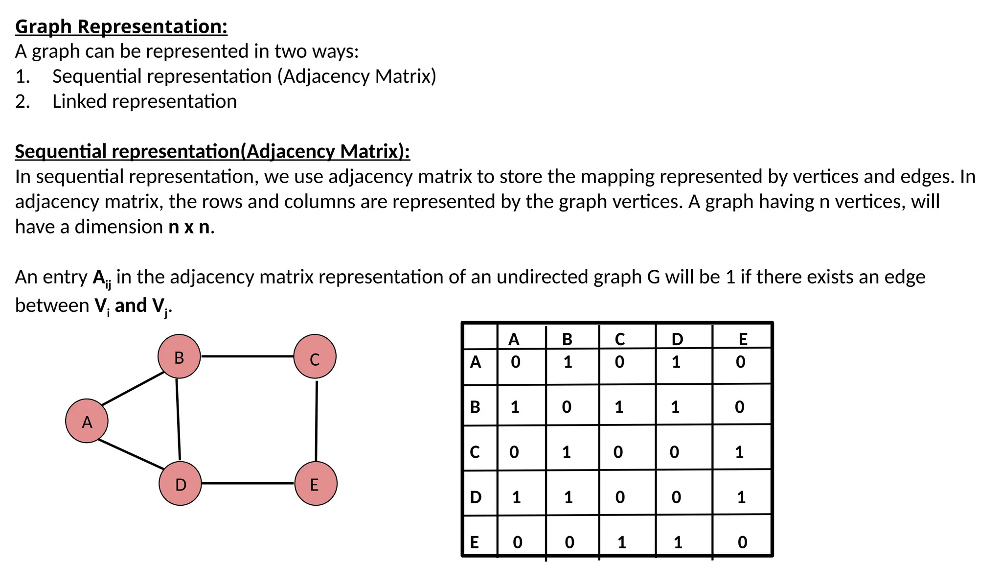
Graph Representation: A graph can be represented in two ways: 1. Sequential representation (Adjacency Matrix) 2. Linked representation Sequential representation(Adjacency Matrix): In sequential representation, we use adjacency matrix to store the mapping represented by vertices and edges. In adjacency matrix, the rows and columns are represented by the graph vertices. A graph having n vertices, will have a dimension n x n. An entry Aij in the adjacency matrix representation of an undirected graph G will be 1 if there exists an edge between Vi and Vj. A B D C E A B C D E A 0 1 0 1 0 B 1 0 1 1 0 C 0 1 0 0 1 D 1 1 0 0 1 E 0 0 1 1 0

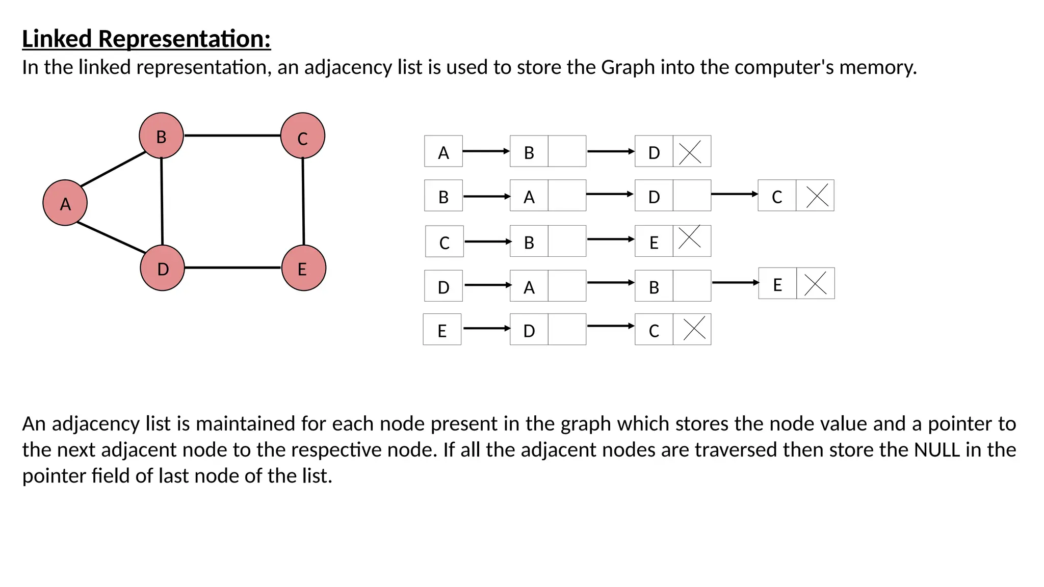
Linked Representation: In the linked representation, an adjacency list is used to store the Graph into the computer's memory. A B D C E A B C D E B D A D B E A B D C C E An adjacency list is maintained for each node present in the graph which stores the node value and a pointer to the next adjacent node to the respective node. If all the adjacent nodes are traversed then store the NULL in the pointer field of last node of the list.

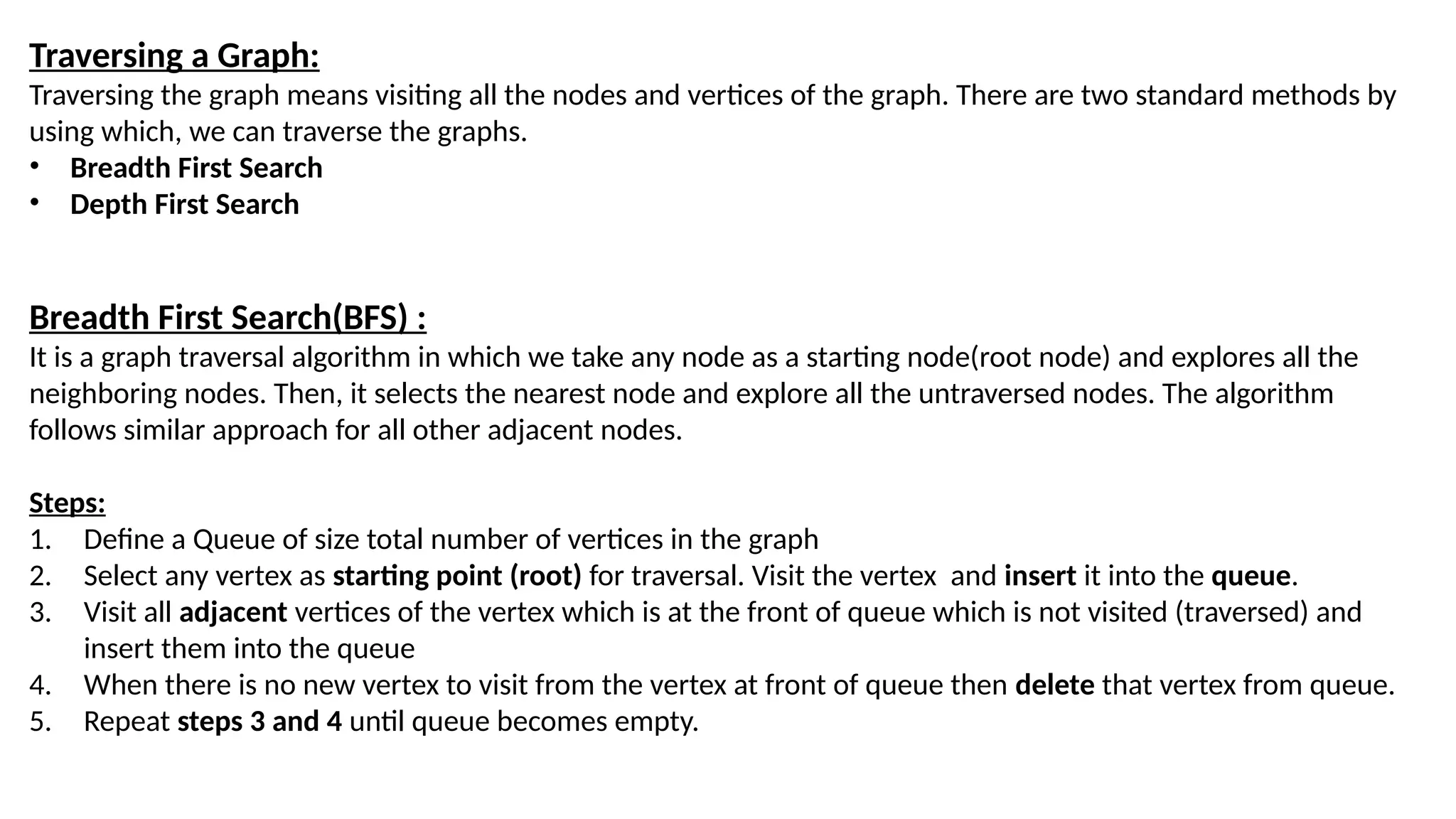
Traversing a Graph: Traversing the graph means visiting all the nodes and vertices of the graph. There are two standard methods by using which, we can traverse the graphs. • Breadth First Search • Depth First Search Breadth First Search(BFS) : It is a graph traversal algorithm in which we take any node as a starting node(root node) and explores all the neighboring nodes. Then, it selects the nearest node and explore all the untraversed nodes. The algorithm follows similar approach for all other adjacent nodes. Steps: 1. Define a Queue of size total number of vertices in the graph 2. Select any vertex as starting point (root) for traversal. Visit the vertex and insert it into the queue. 3. Visit all adjacent vertices of the vertex which is at the front of queue which is not visited (traversed) and insert them into the queue 4. When there is no new vertex to visit from the vertex at front of queue then delete that vertex from queue. 5. Repeat steps 3 and 4 until queue becomes empty.

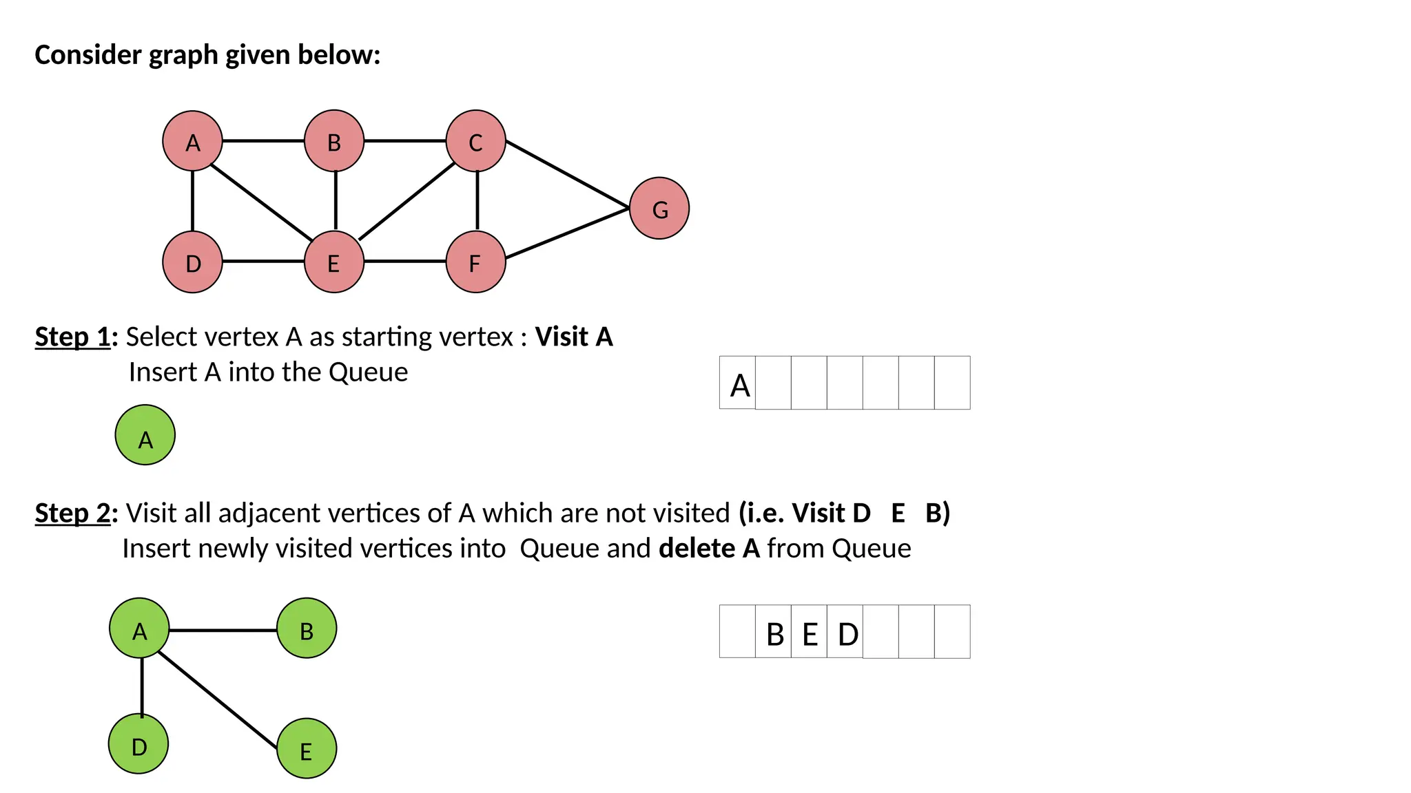
Consider graph given below: Step 1: Select vertex A as starting vertex : Visit A Insert A into the Queue Step 2: Visit all adjacent vertices of A which are not visited (i.e. Visit D E B) Insert newly visited vertices into Queue and delete A from Queue A D B E C F G A A B E D A B E D

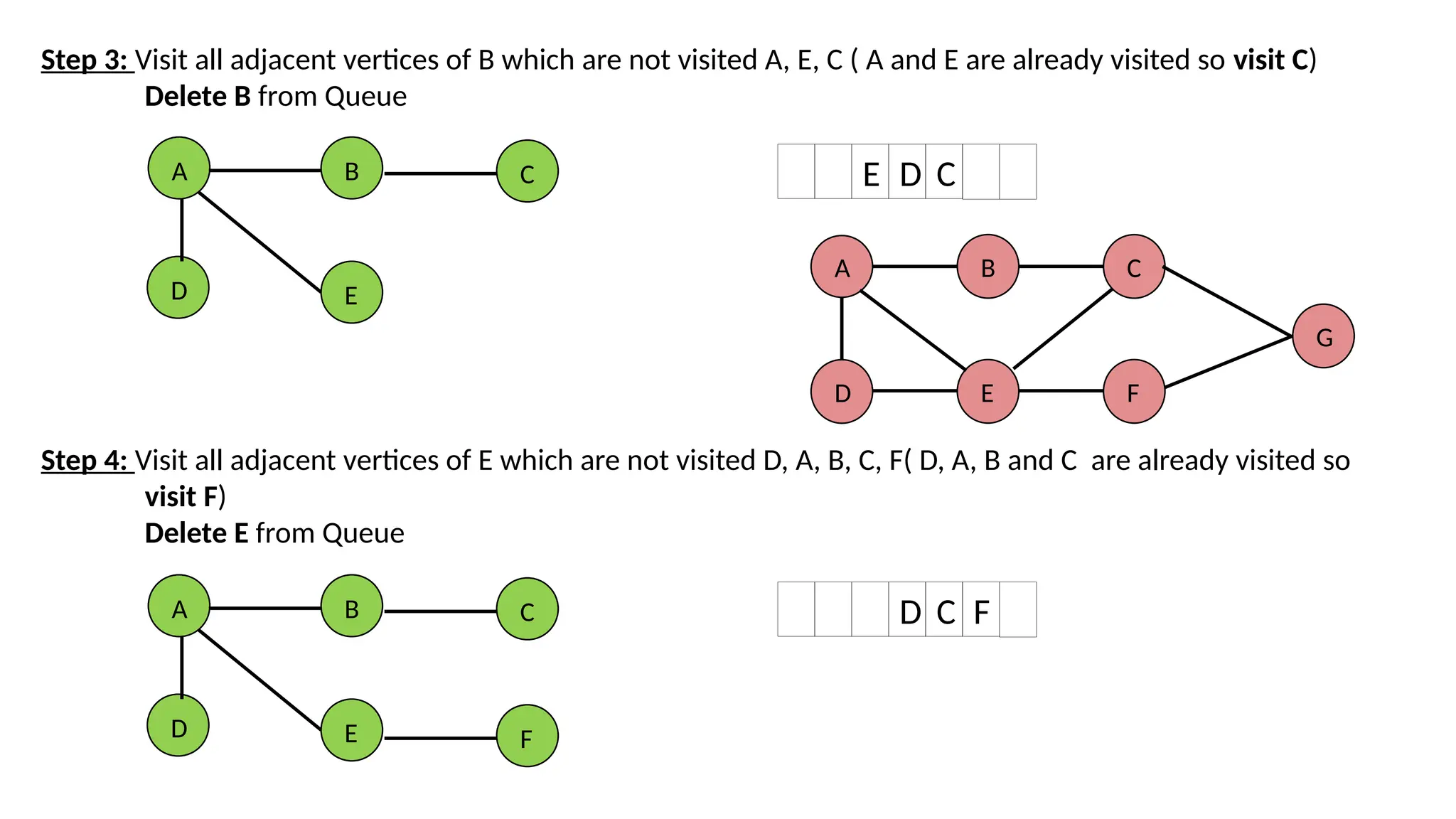
Step 3: Visit all adjacent vertices of B which are not visited A, E, C ( A and E are already visited so visit C) Delete B from Queue Step 4: Visit all adjacent vertices of E which are not visited D, A, B, C, F( D, A, B and C are already visited so visit F) Delete E from Queue E D C A B E D C D C F A B E D C F A D B E C F G

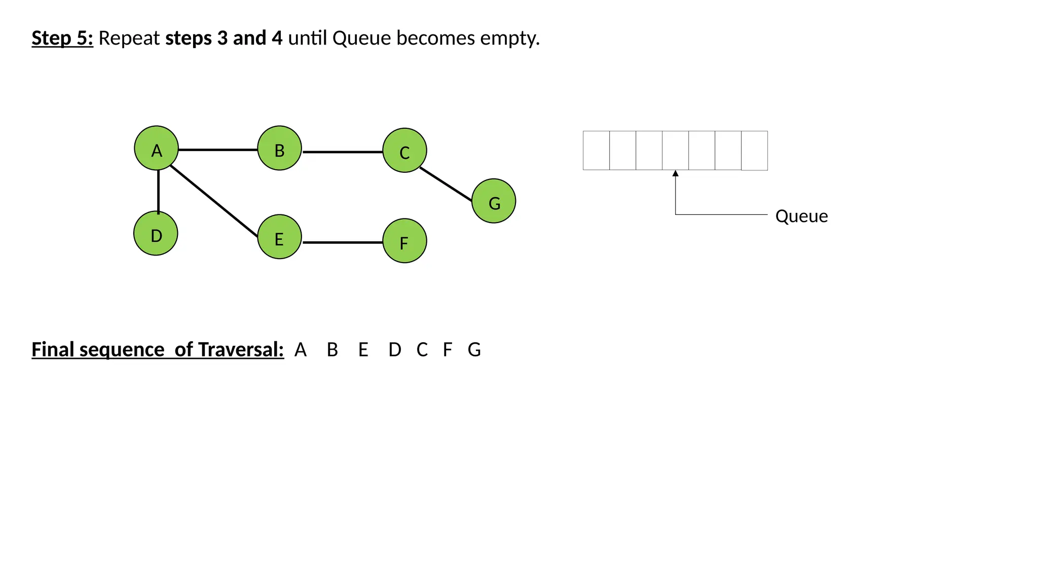
Step 5: Repeat steps 3 and 4 until Queue becomes empty. Final sequence of Traversal: A B E D C F G A B E D C F G Queue

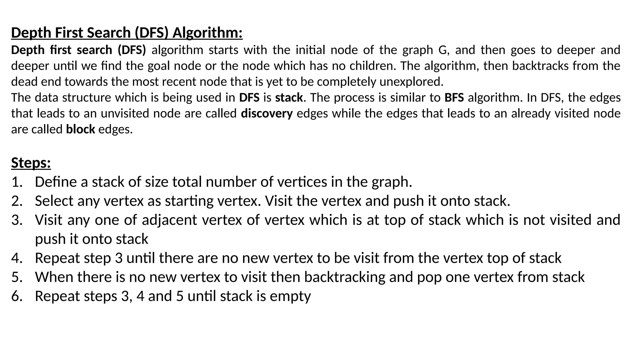
Depth First Search (DFS) Algorithm: Depth first search (DFS) algorithm starts with the initial node of the graph G, and then goes to deeper and deeper until we find the goal node or the node which has no children. The algorithm, then backtracks from the dead end towards the most recent node that is yet to be completely unexplored. The data structure which is being used in DFS is stack. The process is similar to BFS algorithm. In DFS, the edges that leads to an unvisited node are called discovery edges while the edges that leads to an already visited node are called block edges. Steps: 1. Define a stack of size total number of vertices in the graph. 2. Select any vertex as starting vertex. Visit the vertex and push it onto stack. 3. Visit any one of adjacent vertex of vertex which is at top of stack which is not visited and push it onto stack 4. Repeat step 3 until there are no new vertex to be visit from the vertex top of stack 5. When there is no new vertex to visit then backtracking and pop one vertex from stack 6. Repeat steps 3, 4 and 5 until stack is empty

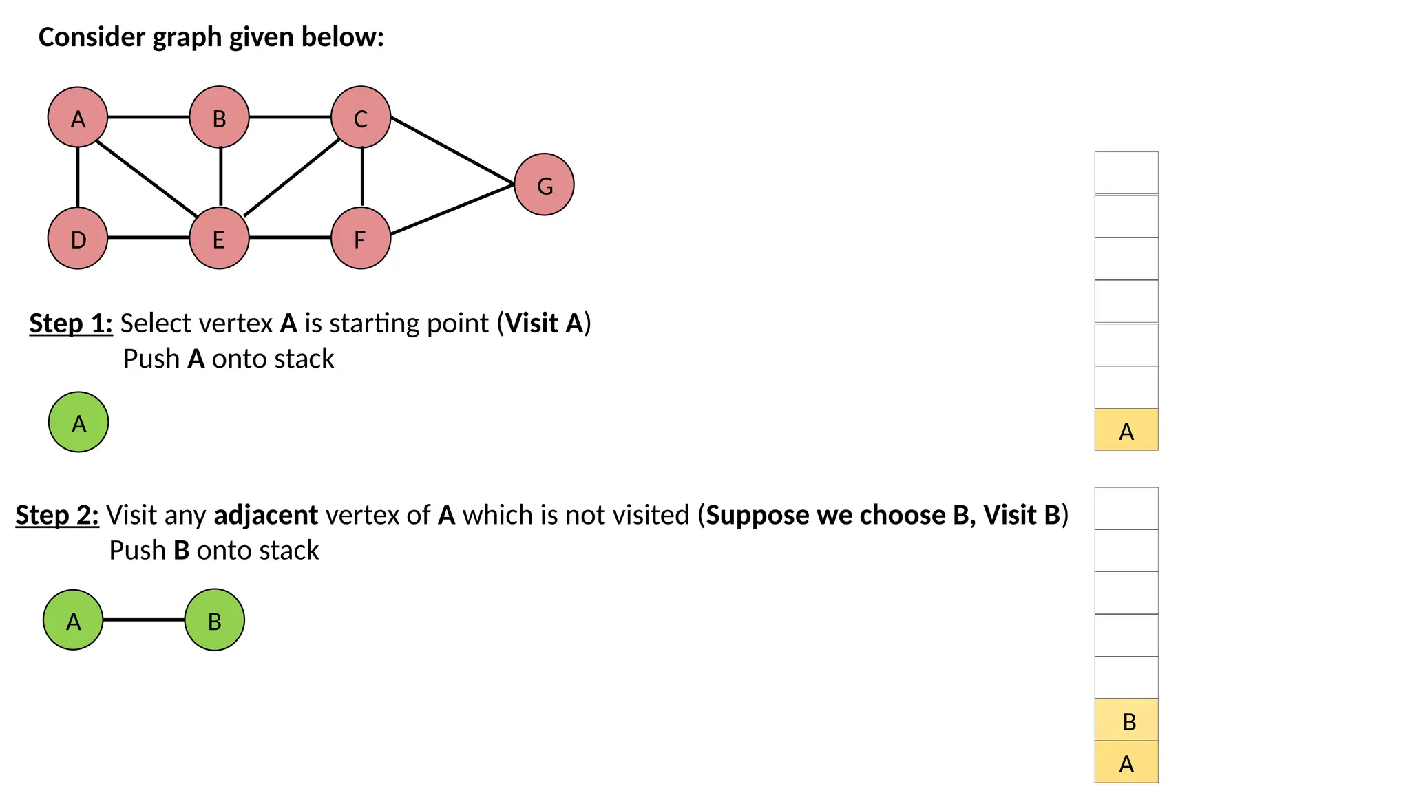
A D B E C F G Consider graph given below: Step 1: Select vertex A is starting point (Visit A) Push A onto stack A A Step 2: Visit any adjacent vertex of A which is not visited (Suppose we choose B, Visit B) Push B onto stack A B A B

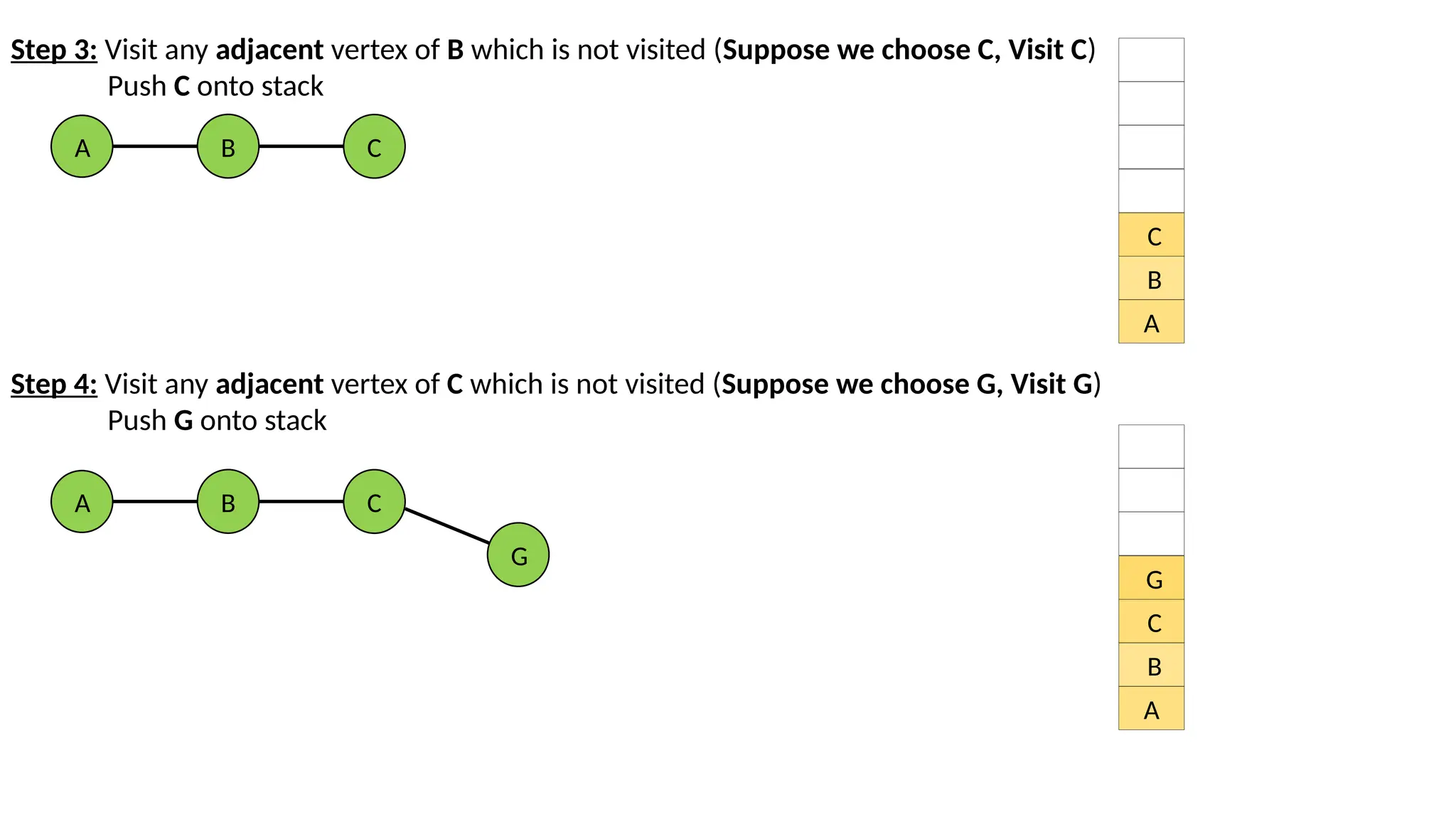
Step 3: Visit any adjacent vertex of B which is not visited (Suppose we choose C, Visit C) Push C onto stack A B C A B C Step 4: Visit any adjacent vertex of C which is not visited (Suppose we choose G, Visit G) Push G onto stack A B C G A B C G

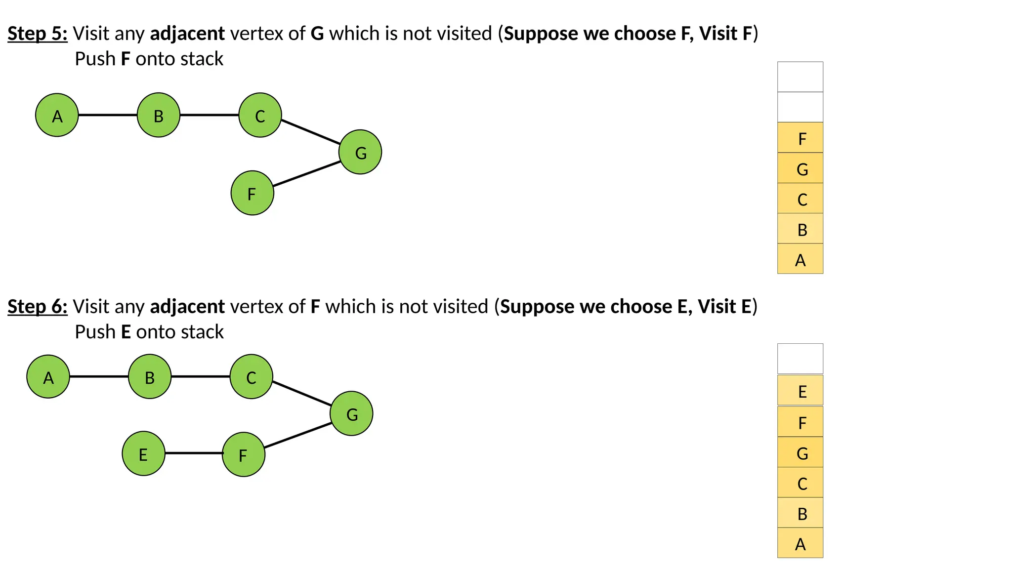
Step 5: Visit any adjacent vertex of G which is not visited (Suppose we choose F, Visit F) Push F onto stack A B C G F A B C G F Step 6: Visit any adjacent vertex of F which is not visited (Suppose we choose E, Visit E) Push E onto stack A B C G F E A B C G F E

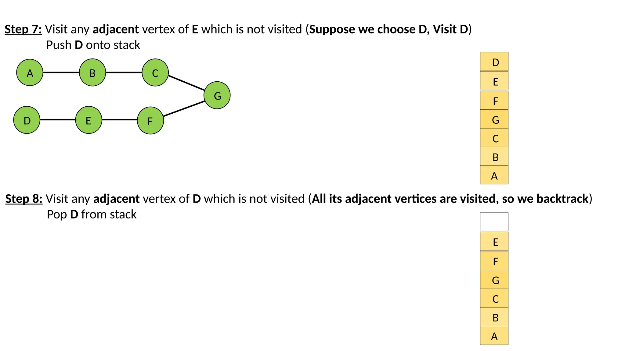
Step 7: Visit any adjacent vertex of E which is not visited (Suppose we choose D, Visit D) Push D onto stack A B C G F E D A B C G F E D Step 8: Visit any adjacent vertex of D which is not visited (All its adjacent vertices are visited, so we backtrack) Pop D from stack A B C G F E

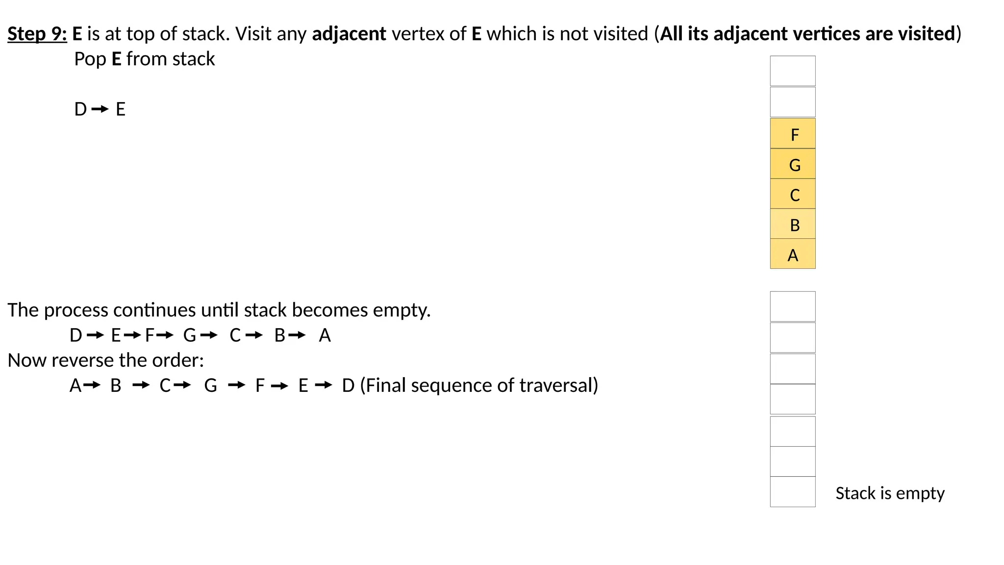
Step 9: E is at top of stack. Visit any adjacent vertex of E which is not visited (All its adjacent vertices are visited) Pop E from stack D E The process continues until stack becomes empty. D E F G C B A Now reverse the order: A B C G F E D (Final sequence of traversal) A B C G F Stack is empty

void BFS(int v) { int i; insert_queue(v); state[v] = waiting; while(!isEmpty_queue()) { v = delete_queue( ); printf("%d ",v); state[v] = visited; for(i=0; i<n; i++) { if(adj[v][i] == 1 && state[i] == initial) { insert_queue(i); state[i] = waiting; } } } printf("n"); } void insert_queue(int vertex) { if(rear == MAX-1) printf("Queue Overflown"); else { if(front == -1) front = 0; rear = rear+1; queue[rear] = vertex ; } }

int isEmpty_queue() { if(front == -1 || front > rear) return 1; else return 0; } int delete_queue() { int delete_item; if(front == -1 || front > rear) { printf("Queue Underflown"); exit(1); } delete_item = queue[front]; front = front+1; return delete_item; }

#include<conio.h> void bfs(int,int); void dfs(int,int); int adj[10][10],visited[10]; void main() { int i,j,n,s,ch; clrscr(); printf("nEnter number of vertices:"); scanf("%d",&n); printf("nEnter adjacency matrix:"); for(i=1;i<=n;i++) { for(j=1;j<=n;j++) { scanf("%d",&adj[i][j]); } } A B D C E F G 1 2 4 3 5 6 7

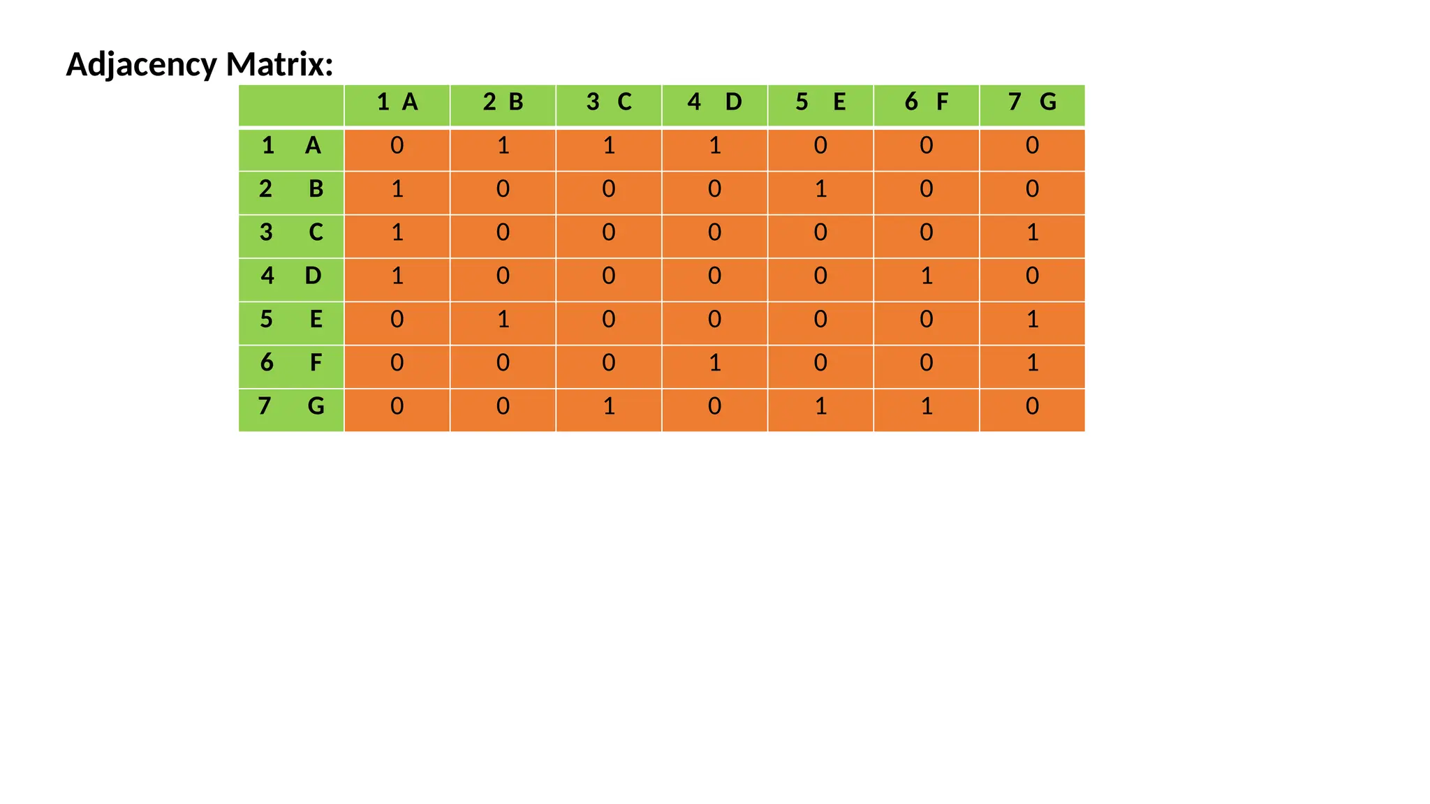
Adjacency Matrix: 1 A 2 B 3 C 4 D 5 E 6 F 7 G 1 A 0 1 1 1 0 0 0 2 B 1 0 0 0 1 0 0 3 C 1 0 0 0 0 0 1 4 D 1 0 0 0 0 1 0 5 E 0 1 0 0 0 0 1 6 F 0 0 0 1 0 0 1 7 G 0 0 1 0 1 1 0

printf("nAdjacency matrix:n"); for(i=1;i<=n;i++) { for(j=1;j<=n;j++) { printf("%d ",adj[i][j]); } printf("n"); } for(i=1;i<=n;i++) visited[i]=0; printf("nEnter source vertex:"); scanf("%d",&s); printf("nEnter your choicen 1. BFS n2. DFSn"); scanf("%d",&ch); switch(ch) { case 1: bfs(s,n); break; case 2: dfs(s,n); break; } }

/*bfs*/ void bfs(int s,int n) { int i,f=-1,r=-1,q[10]; printf("nBFS traversal: "); printf("n%d",s); visited[s]=1; r++; f++; q[r]=s; while(f<=r) { s=q[f]; f++; for(i=1;i<=n;i++) { if(adj[s][i]==1 && visited[i]==0) { printf(" %d",i); visited[i]=1; r++; q[r]=i; } } } }

/*dfs*/ void dfs(int s,int n) { int i,st[10],top=-1,pop,j,k; printf("nDFS traversal:"); top++; st[top]=s; while(top>=0) { pop=st[top]; top--; if(visited[pop]==0) { printf("%d ",pop); visited[pop]=1; } else continue; for(i=n;i>=1;i--) { if(adj[pop][i]==1 && visited[i]==0) { top++; st[top]=i; } } } }

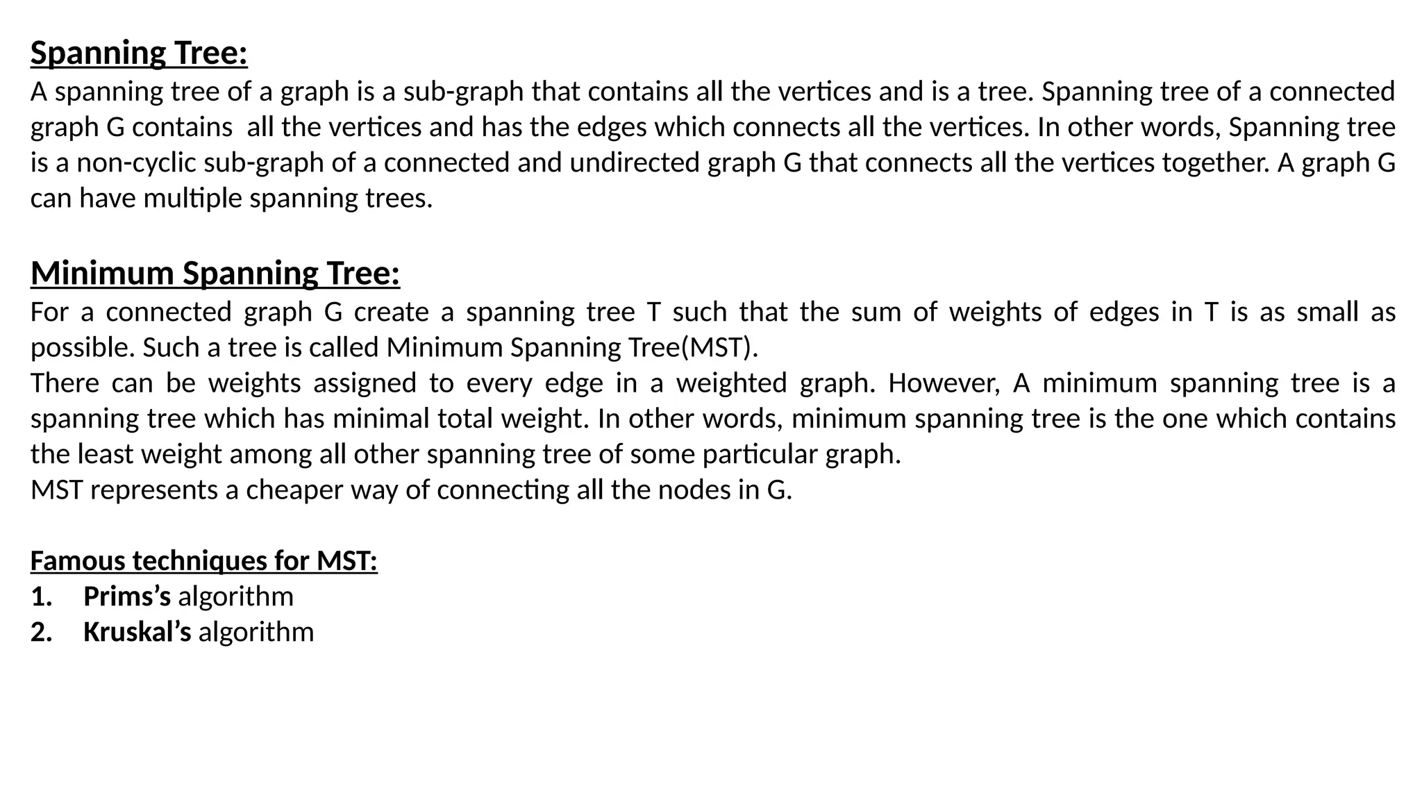
Spanning Tree: A spanning tree of a graph is a sub-graph that contains all the vertices and is a tree. Spanning tree of a connected graph G contains all the vertices and has the edges which connects all the vertices. In other words, Spanning tree is a non-cyclic sub-graph of a connected and undirected graph G that connects all the vertices together. A graph G can have multiple spanning trees. Minimum Spanning Tree: For a connected graph G create a spanning tree T such that the sum of weights of edges in T is as small as possible. Such a tree is called Minimum Spanning Tree(MST). There can be weights assigned to every edge in a weighted graph. However, A minimum spanning tree is a spanning tree which has minimal total weight. In other words, minimum spanning tree is the one which contains the least weight among all other spanning tree of some particular graph. MST represents a cheaper way of connecting all the nodes in G. Famous techniques for MST: 1. Prims’s algorithm 2. Kruskal’s algorithm

Prim's Algorithm: Prim's Algorithm is used to find the minimum spanning tree from a graph. Prim's algorithm finds the subset of edges that includes every vertex of the graph such that the sum of the weights of the edges can be minimized. Prim's algorithm starts with the single node and explore all the adjacent nodes with all the connecting edges at every step. The edges with the minimal weights causing no cycles in the graph got selected. Prim’s algorithm has the property that the edges in always forms a single tree. Begin with some vertex U in the graph G. in each iteration we choose the minimum weight edge (U,V) connecting a vertex V in the set A to the vertex U outside to set A. Then vertex U is bought into A. This process is repeated until a spanning tree is formed. Algorithm 1. Select a starting vertex 2. Repeat Steps 3 and 4 until there are fringe vertices 3. Select an edge e connecting the tree vertex and fringe vertex that has minimum weight 4.Add the selected edge and the vertex to the minimum spanning tree T [END OF LOOP] 5. EXIT

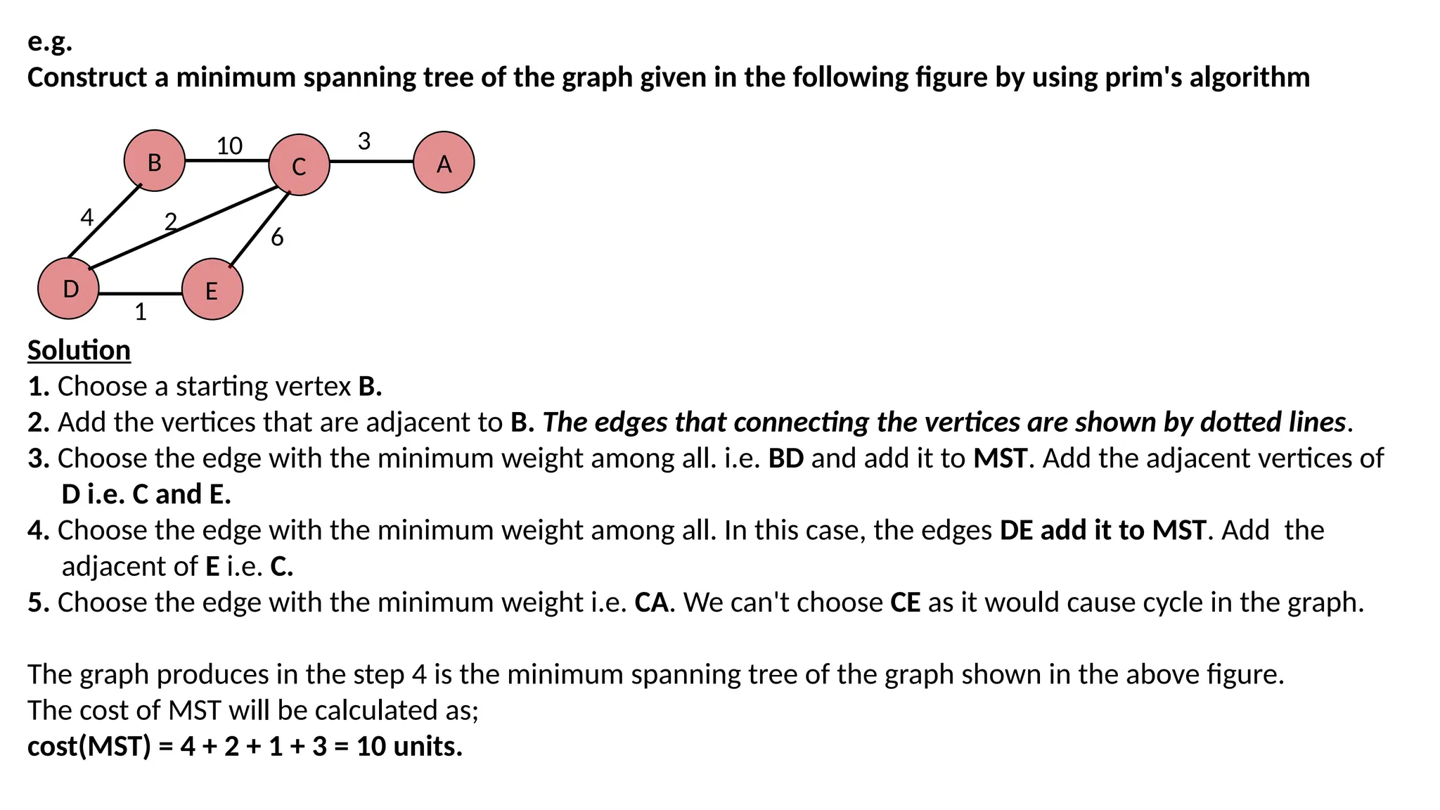
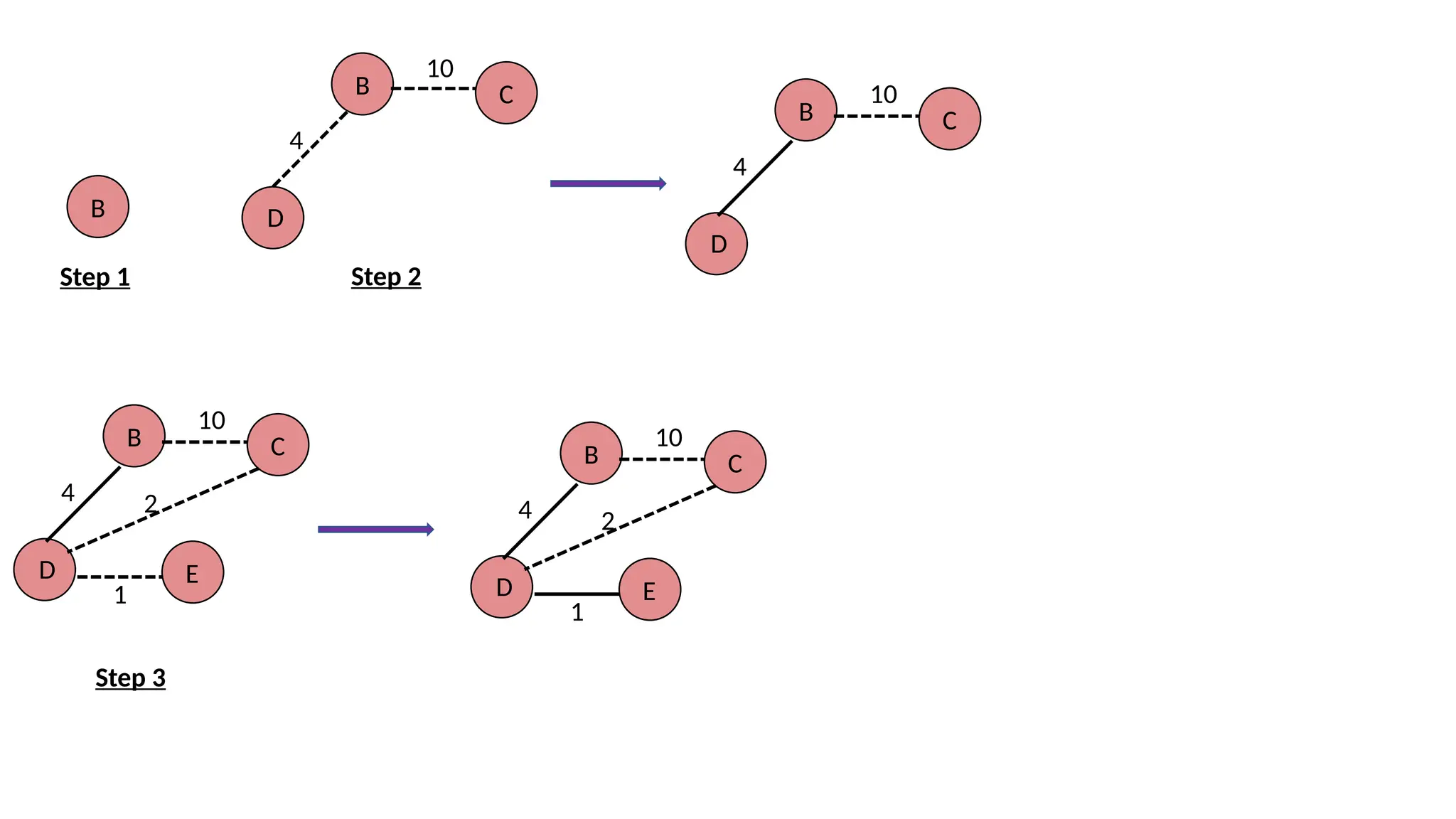
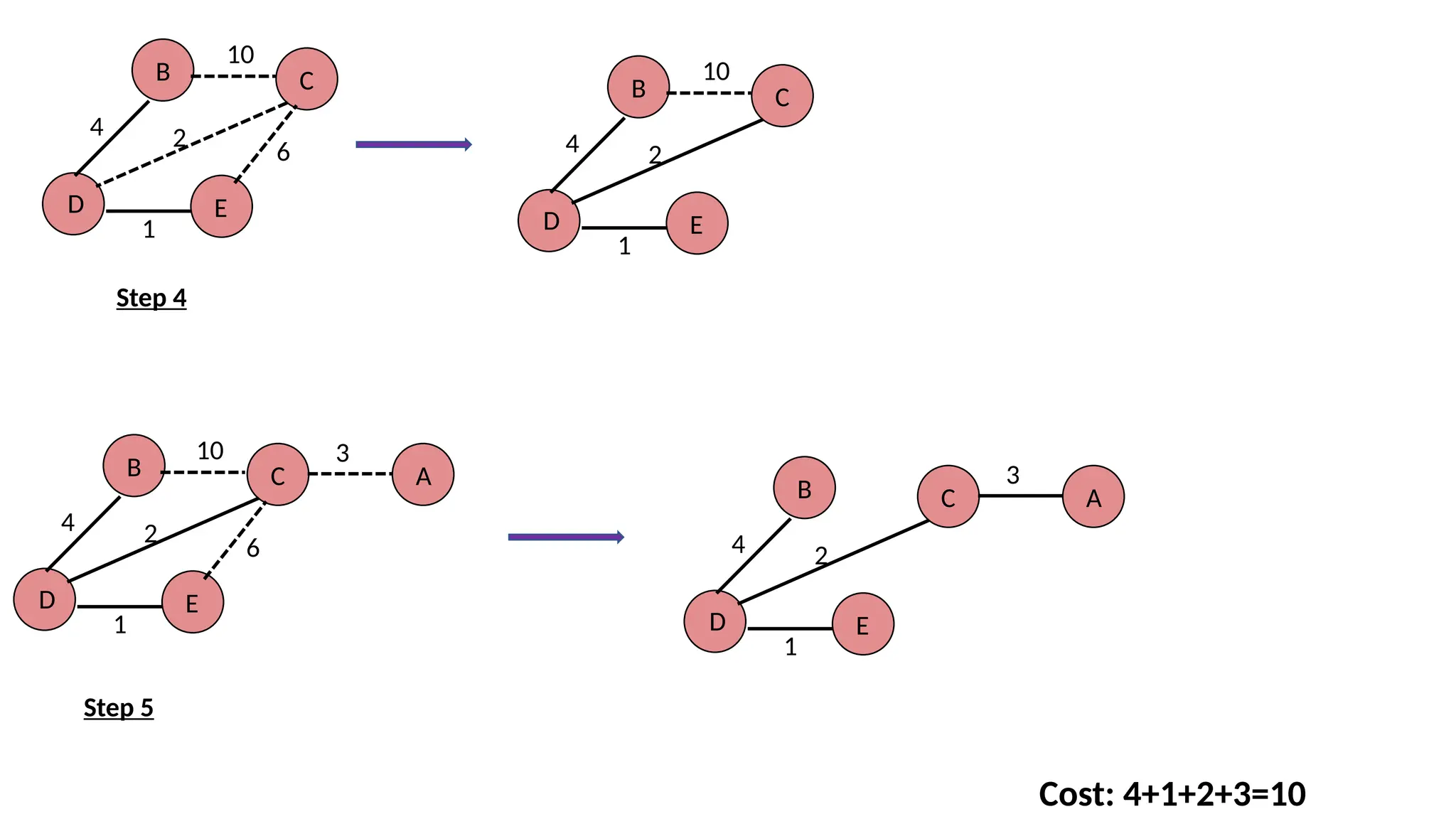
e.g. Construct a minimum spanning tree of the graph given in the following figure by using prim's algorithm B D C E A 10 3 6 1 2 4 Solution 1. Choose a starting vertex B. 2. Add the vertices that are adjacent to B. The edges that connecting the vertices are shown by dotted lines. 3. Choose the edge with the minimum weight among all. i.e. BD and add it to MST. Add the adjacent vertices of D i.e. C and E. 4. Choose the edge with the minimum weight among all. In this case, the edges DE add it to MST. Add the adjacent of E i.e. C. 5. Choose the edge with the minimum weight i.e. CA. We can't choose CE as it would cause cycle in the graph. The graph produces in the step 4 is the minimum spanning tree of the graph shown in the above figure. The cost of MST will be calculated as; cost(MST) = 4 + 2 + 1 + 3 = 10 units.

B Step 1 B D C Step 2 10 4 B D C 10 4 B D C 10 4 E 1 2 Step 3 B D C 10 4 E 1 2

B D C 10 4 E 1 2 6 Step 4 B D C 10 4 E 1 2 B D C 4 E 1 2 Step 5 A 3 B D C 4 E 1 2 A 3 10 6 Cost: 4+1+2+3=10

/*program for the implementation of prims algorithm*/ #include<stdio.h> #include<conio.h> int i,j,a,b,u,v,n,ne=1; int min,mincost=0,cost[10][10],visited[10]={0}; void prims(); void main() { clrscr(); printf("nEnter number of vertices:"); scanf("%d",&n); printf("nEnter cost adjacency matrix:"); for(i=1;i<=n;i++) { for(j=1;j<=n;j++) { scanf("%d",&cost[i][j]); if(cost[i][j]==0) cost[i][j]=999; } } printf("nCost Adjacency matrix:n"); for(i=1;i<=n;i++) { for(j=1;j<=n;j++) { printf("%d ",cost[i][j]); } printf("n"); } prims(); getch(); }

/*prims function*/ void prims() { visited[1]=1; while(ne<n) { for(i=1,min=999;i<=n;i++) for(j=1;j<=n;j++) if(cost[i][j]<min) if(visited[i]!=0) { min=cost[i][j]; a=u=i; b=v=j; } if(visited[u]==0 || visited[v]==0) { printf("n%d edge (%d,%d)=%d",ne++,a,b,min); mincost+=min; visited[b]=1; } cost[a][b]=cost[b][a]=999; } printf("nMinimum cost=%d",mincost); }

Kruskal's Algorithm: Kruskal's Algorithm is used to find the minimum spanning tree for a connected weighted graph. The main target of the algorithm is to find the subset of edges by using which, we can traverse every vertex of the graph. Kruskal's algorithm follows greedy approach which finds an optimum solution at every stage instead of focusing on a global optimum. The algorithm creates a forest of trees. The forest consists of n-single nodes trees and no edges. At each step, we add one (cheapest one) edge , so that it joins two trees together. Algorithm 1. Create a forest in such a way that each graph is a separate tree. 2. Create a priority queue Q that contains all the edges of the graph. 3. Repeat Steps 4 and 5 while Q is NOT EMPTY 4. Remove an edge from Q 5. IF the edge obtained in Step 4 connects two different trees, then Add it to the forest (for combining two trees into one tree). ELSE Discard the edge 6. END

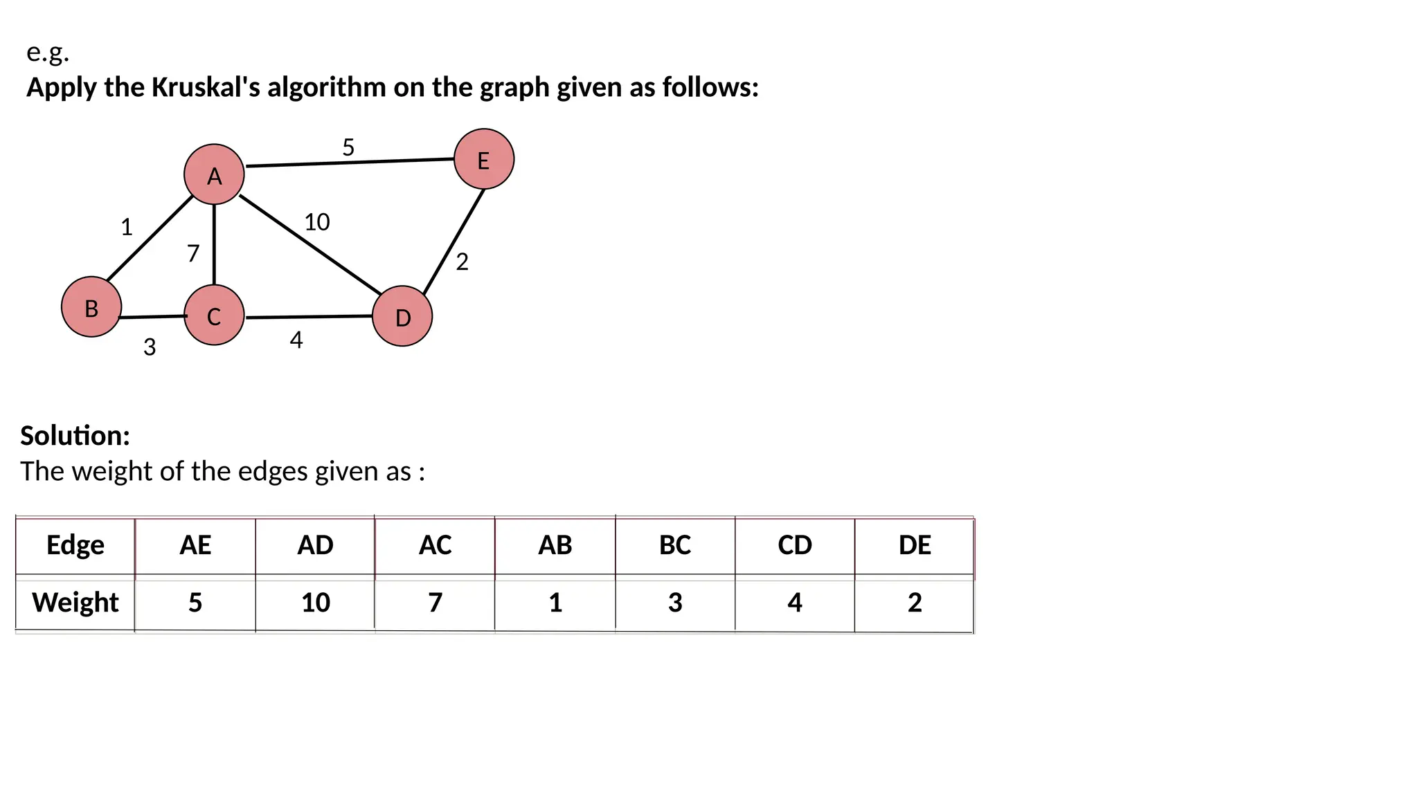
e.g. Apply the Kruskal's algorithm on the graph given as follows: A B C D E 1 3 7 10 4 2 5 Solution: The weight of the edges given as : Edge AE AD AC AB BC CD DE Weight 5 10 7 1 3 4 2

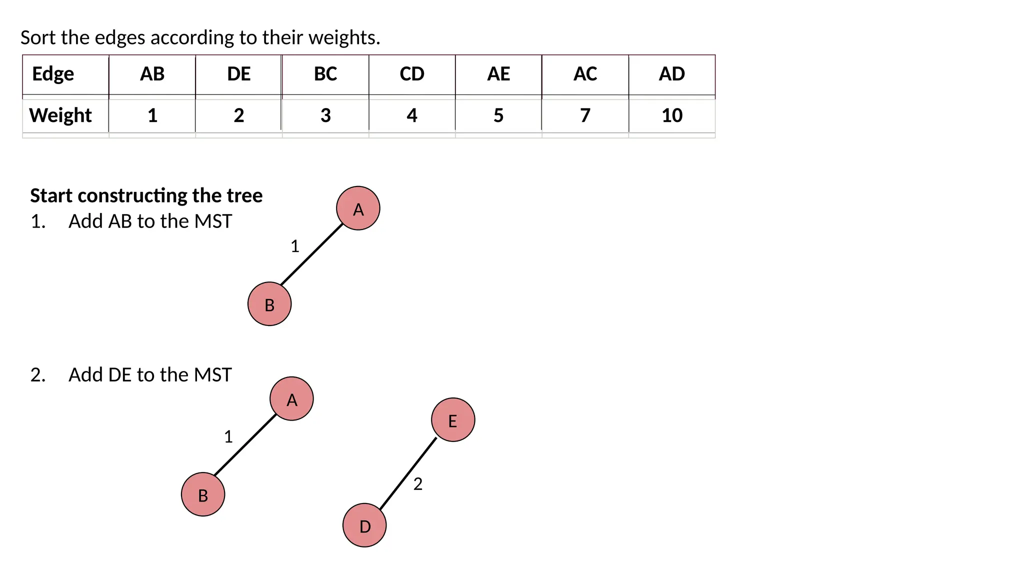
Sort the edges according to their weights. Edge AB DE BC CD AE AC AD Weight 1 2 3 4 5 7 10 Start constructing the tree 1. Add AB to the MST 2. Add DE to the MST A B 1 A B 1 D E 2

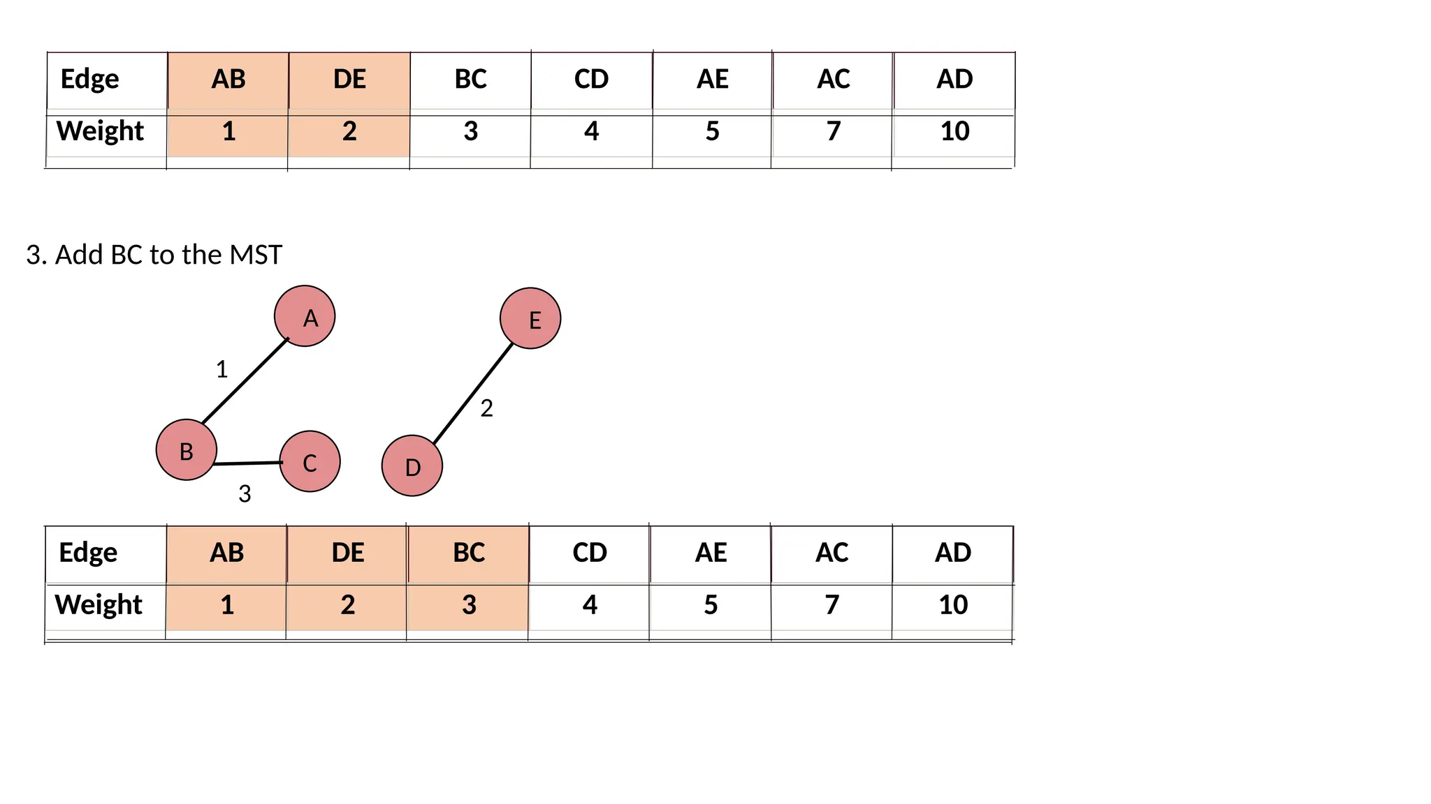
Edge AB DE BC CD AE AC AD Weight 1 2 3 4 5 7 10 Edge AB DE BC CD AE AC AD Weight 1 2 3 4 5 7 10 3. Add BC to the MST A B 1 D E 2 C 3

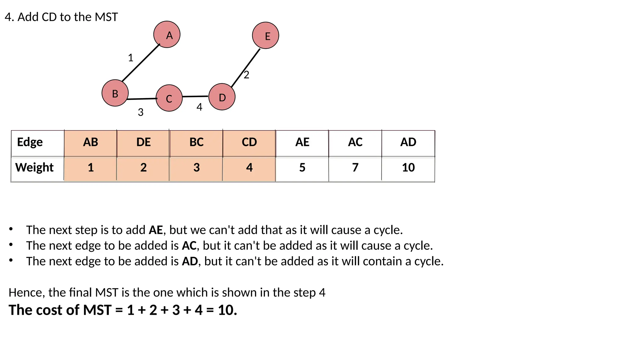
4. Add CD to the MST A B 1 D E 2 C 3 4 Edge AB DE BC CD AE AC AD Weight 1 2 3 4 5 7 10 • The next step is to add AE, but we can't add that as it will cause a cycle. • The next edge to be added is AC, but it can't be added as it will cause a cycle. • The next edge to be added is AD, but it can't be added as it will contain a cycle. Hence, the final MST is the one which is shown in the step 4 The cost of MST = 1 + 2 + 3 + 4 = 10.

/*program for the implementation of kruskals algorithm*/ #include<stdio.h> #include<conio.h> int i,j,k,a,b,u,v,n,ne=1; int min,mincost=0,cost[10][10],parent[10]; int find(int); void kruskal(); int uni(int,int); void main() { printf("nEnter number of vertices:"); scanf("%d",&n); printf("nEnter cost adjacency matrix:"); for(i=1;i<=n;i++) { for(j=1;j<=n;j++) { scanf("%d",&cost[i][j]); if(cost[i][j]==0) cost[i][j]=999; } } printf("nCost Adjacency matrix:n"); for(i=1;i<=n;i++) { for(j=1;j<=n;j++) { printf("%d ",cost[i][j]); } printf("n"); } kruskal(); getch(); }

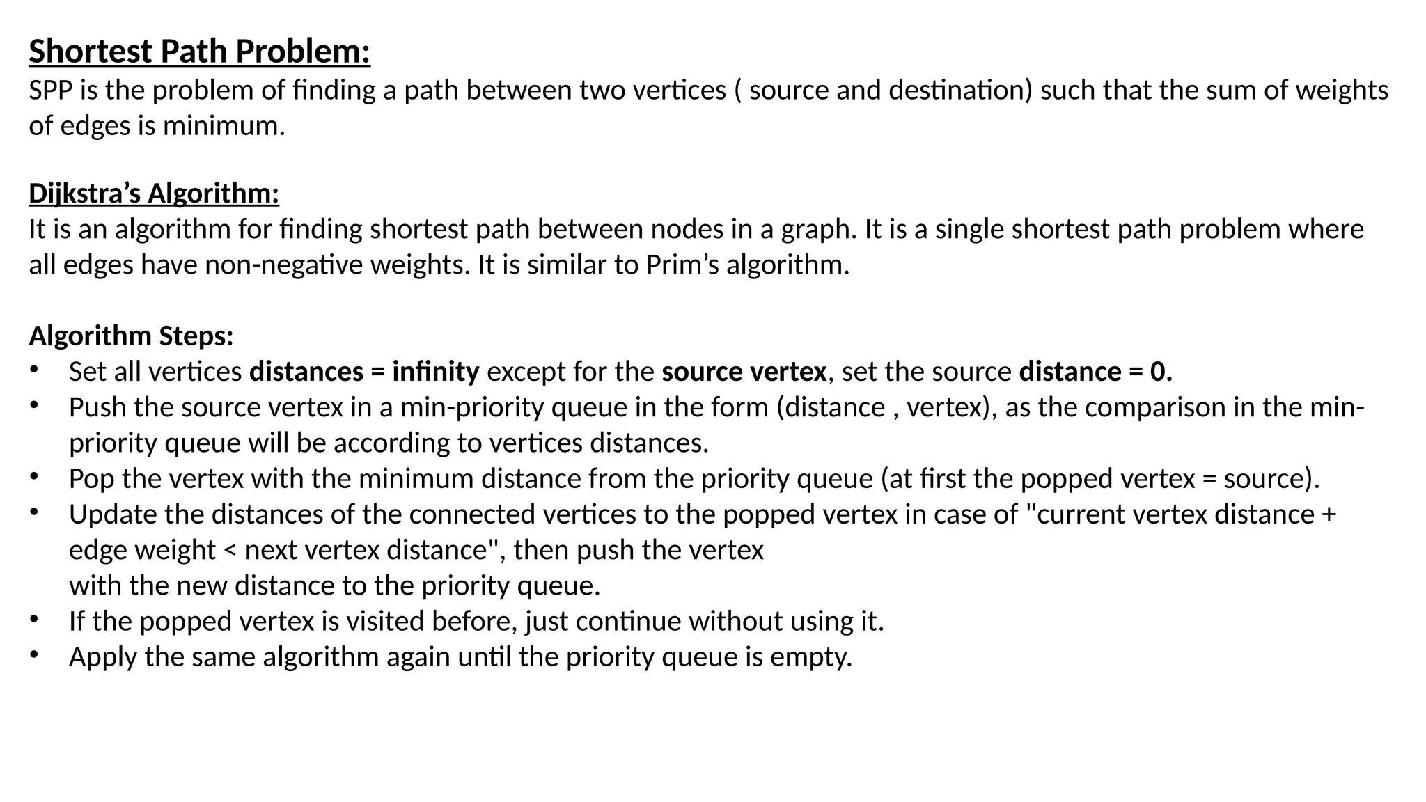
/*kruskal function*/ void kruskal() { while(ne<n) { for(i=1,min=999;i<=n;i++) { for(j=1;j<=n;j++) { if(cost[i][j]<min) { min=cost[i][j]; a=u=i; b=v=j; } } } u=find(u); v=find(v); if(uni(u,v)) { printf("n%d edge (%d,%d)=%d",ne++,a,b,min); mincost+=min; } cost[a][b]=cost[b][a]=999; } printf("nMinimum cost=%d",mincost); }

/*find function*/ int find(int i) { while(parent[i]) i=parent[i]; return i; } /*union function*/ int uni(int i,int j) { if(i!=j) { parent[j]=i; return 1; } return 0; }

Shortest Path Problem: SPP is the problem of finding a path between two vertices ( source and destination) such that the sum of weights of edges is minimum. Dijkstra’s Algorithm: It is an algorithm for finding shortest path between nodes in a graph. It is a single shortest path problem where all edges have non-negative weights. It is similar to Prim’s algorithm. Algorithm Steps: • Set all vertices distances = infinity except for the source vertex, set the source distance = 0. • Push the source vertex in a min-priority queue in the form (distance , vertex), as the comparison in the min- priority queue will be according to vertices distances. • Pop the vertex with the minimum distance from the priority queue (at first the popped vertex = source). • Update the distances of the connected vertices to the popped vertex in case of "current vertex distance + edge weight < next vertex distance", then push the vertex with the new distance to the priority queue. • If the popped vertex is visited before, just continue without using it. • Apply the same algorithm again until the priority queue is empty.

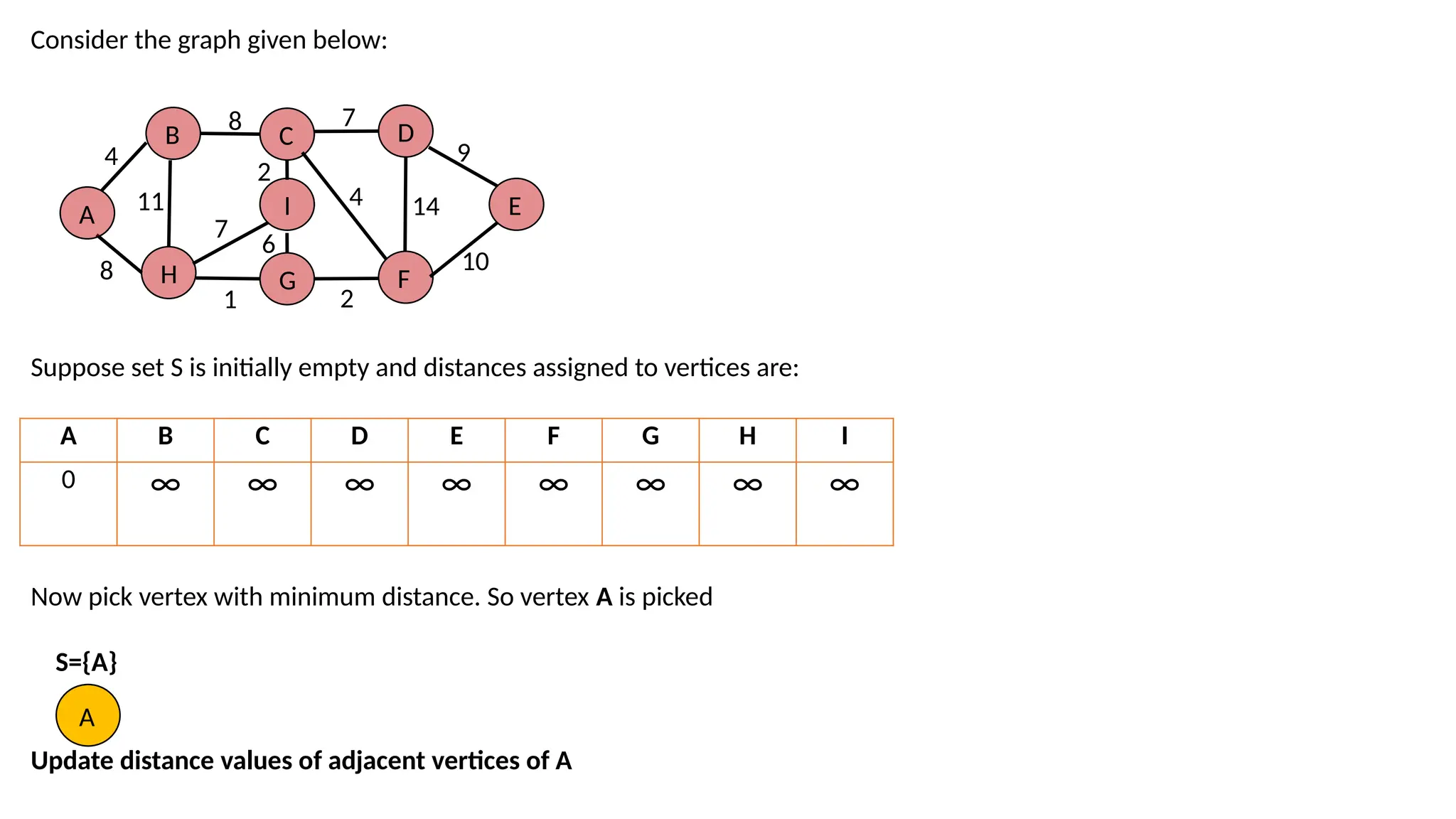
Consider the graph given below: Suppose set S is initially empty and distances assigned to vertices are: Now pick vertex with minimum distance. So vertex A is picked S={A} Update distance values of adjacent vertices of A A B H G C I D F E 4 8 11 8 7 2 6 1 4 2 7 9 14 10 A B C D E F G H I 0 ∞ ∞ ∞ ∞ ∞ ∞ ∞ ∞ A

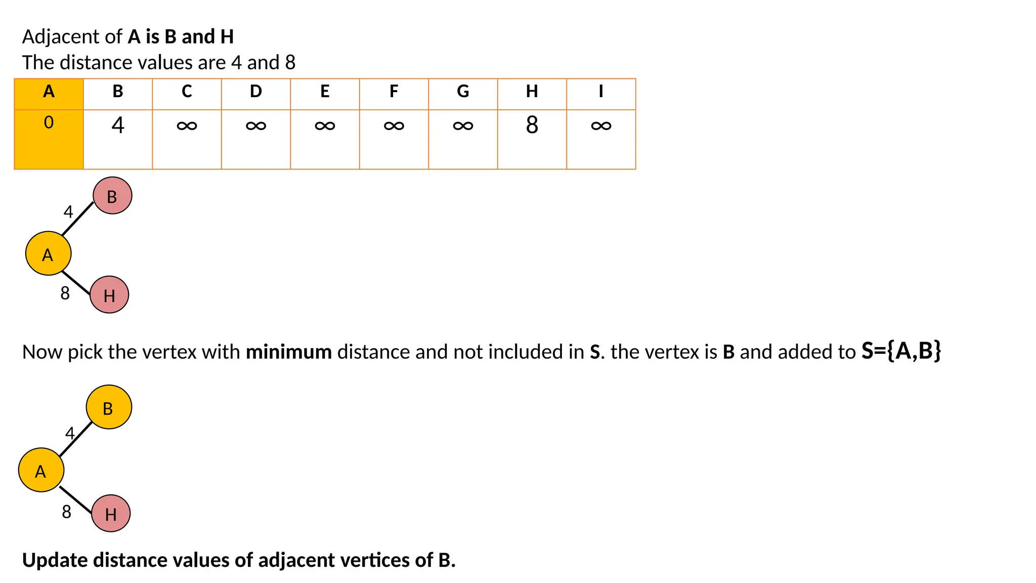
Adjacent of A is B and H The distance values are 4 and 8 Now pick the vertex with minimum distance and not included in S. the vertex is B and added to S={A,B} Update distance values of adjacent vertices of B. A B C D E F G H I 0 4 ∞ ∞ ∞ ∞ ∞ 8 ∞ B H 4 8 A A B H 4 8

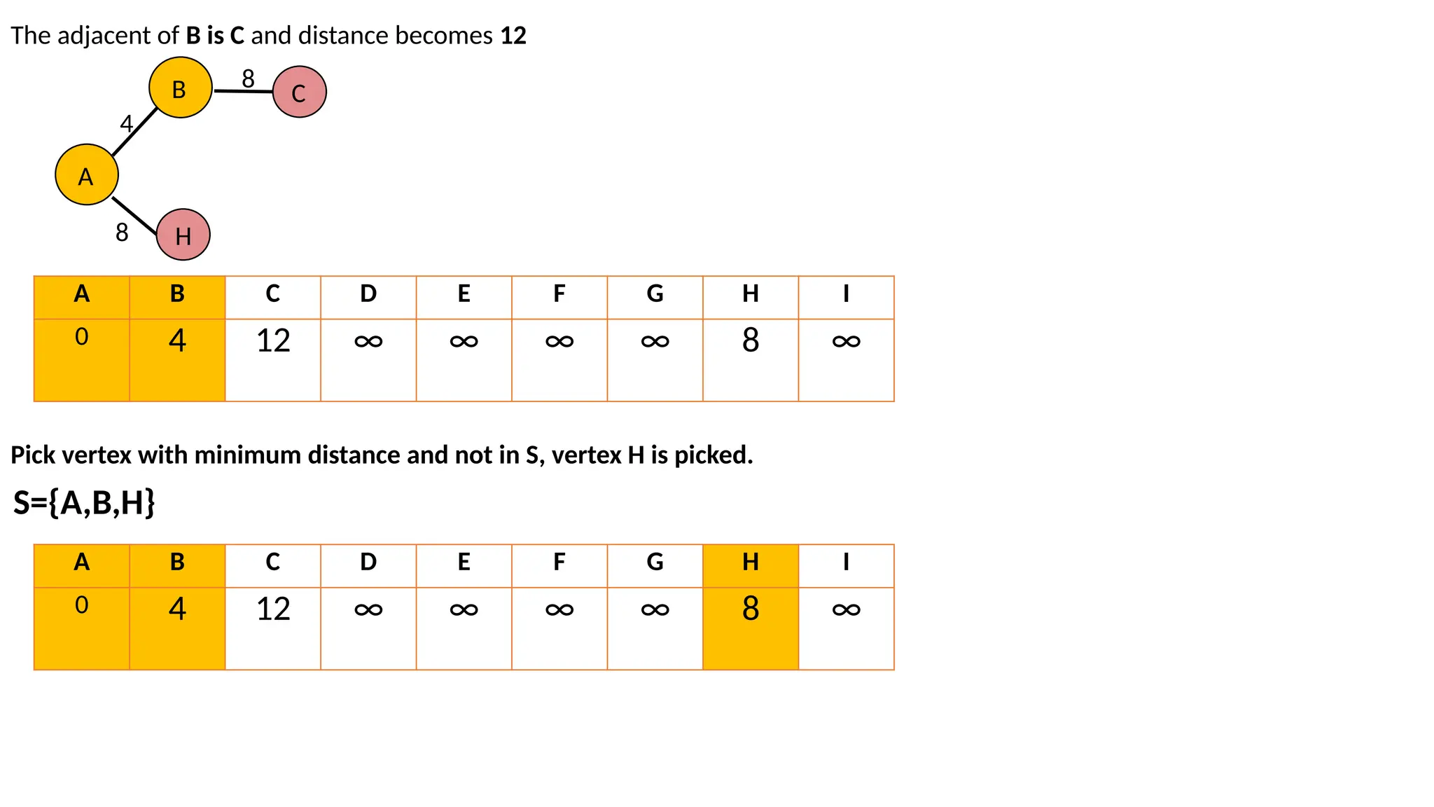
The adjacent of B is C and distance becomes 12 Pick vertex with minimum distance and not in S, vertex H is picked. A B H 4 8 C 8 A B C D E F G H I 0 4 12 ∞ ∞ ∞ ∞ 8 ∞ S={A,B,H} A B C D E F G H I 0 4 12 ∞ ∞ ∞ ∞ 8 ∞

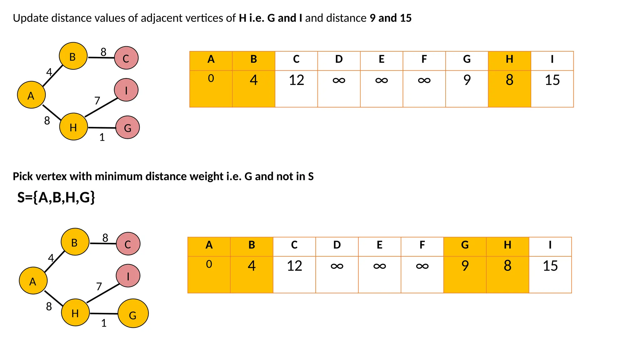
Update distance values of adjacent vertices of H i.e. G and I and distance 9 and 15 Pick vertex with minimum distance weight i.e. G and not in S A B 4 8 C 8 H G I 7 1 A B C D E F G H I 0 4 12 ∞ ∞ ∞ 9 8 15 S={A,B,H,G} A B 4 8 C 8 H G I 7 1 A B C D E F G H I 0 4 12 ∞ ∞ ∞ 9 8 15

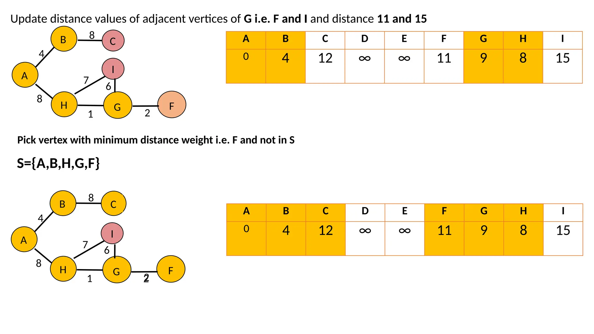
Update distance values of adjacent vertices of G i.e. F and I and distance 11 and 15 A B C D E F G H I 0 4 12 ∞ ∞ 11 9 8 15 Pick vertex with minimum distance weight i.e. F and not in S S={A,B,H,G,F} A B 4 8 C 8 H G I 7 1 F 6 2 A B 4 8 C 8 H G I 7 1 F 2 2 6 A B C D E F G H I 0 4 12 ∞ ∞ 11 9 8 15

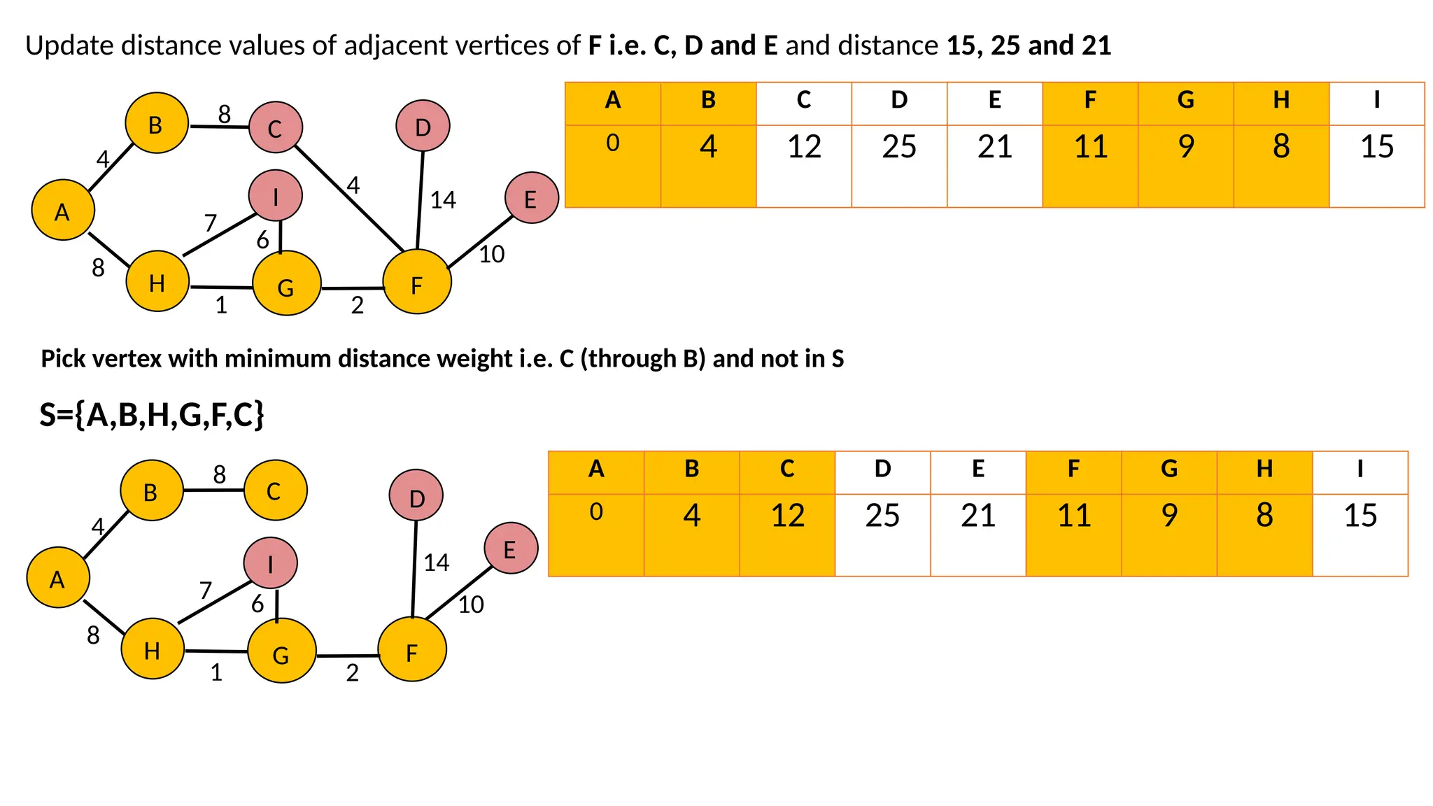
Update distance values of adjacent vertices of F i.e. C, D and E and distance 15, 25 and 21 A B 4 8 C 8 H G I 7 1 F 2 A B 4 8 C 8 H G I 7 1 F 2 6 6 D E 4 14 10 A B C D E F G H I 0 4 12 25 21 11 9 8 15 Pick vertex with minimum distance weight i.e. C (through B) and not in S S={A,B,H,G,F,C} A B C D E F G H I 0 4 12 25 21 11 9 8 15 D E 14 10

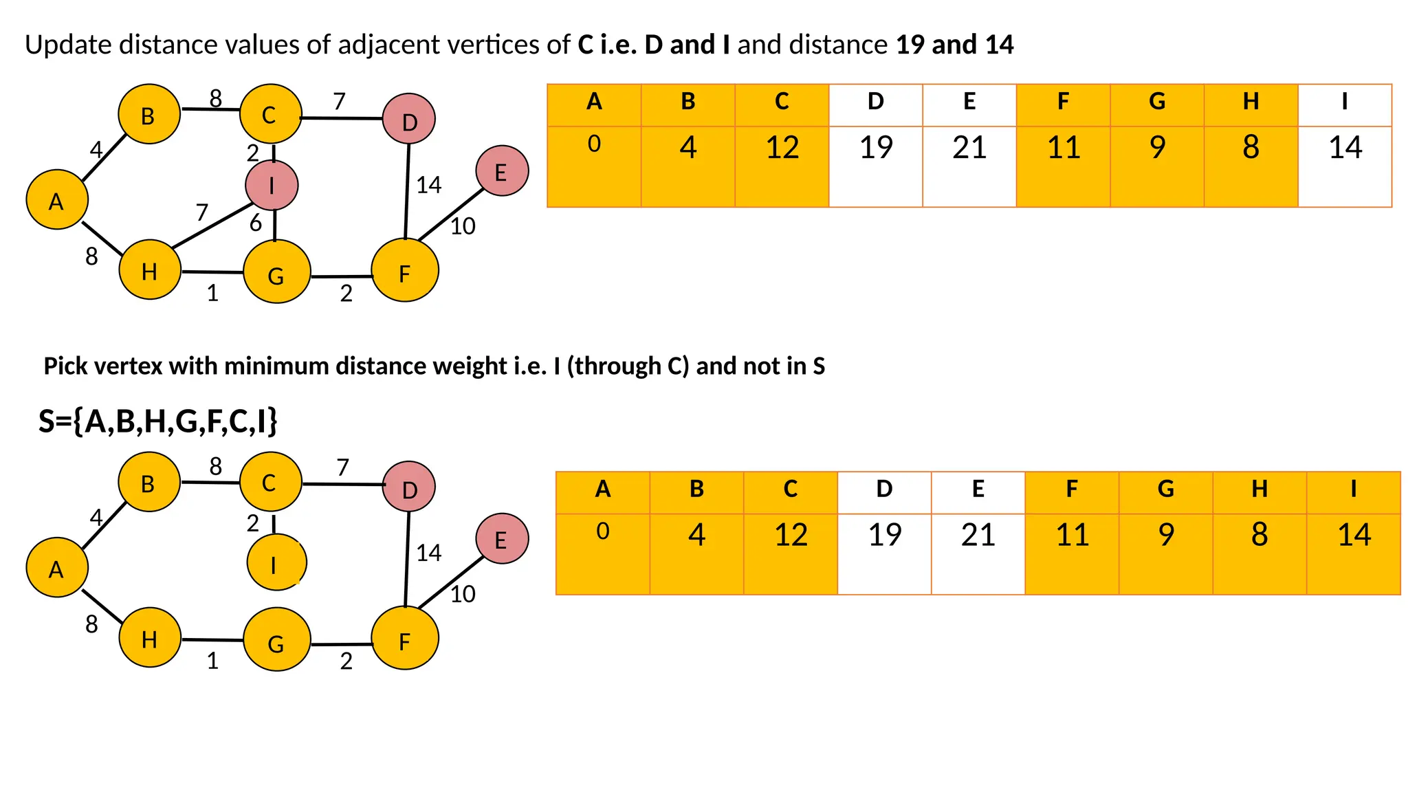
Update distance values of adjacent vertices of C i.e. D and I and distance 19 and 14 A B 4 8 C 8 H G I 1 F 2 D E 14 10 A B 4 8 C 8 H G I 7 1 F 2 D E 14 10 6 2 7 A B C D E F G H I 0 4 12 19 21 11 9 8 14 Pick vertex with minimum distance weight i.e. I (through C) and not in S S={A,B,H,G,F,C,I} 2 A B C D E F G H I 0 4 12 19 21 11 9 8 14 7

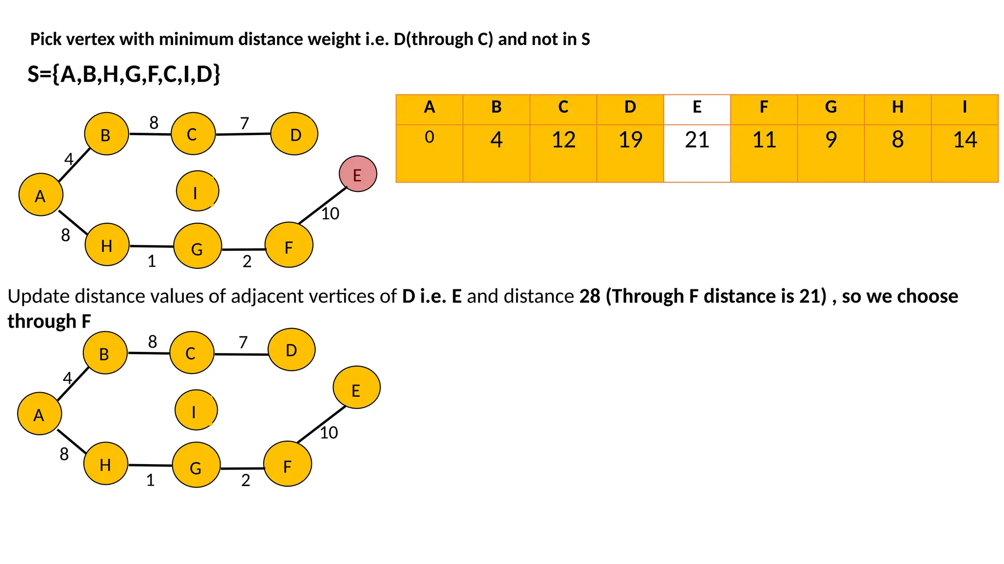
Pick vertex with minimum distance weight i.e. D(through C) and not in S S={A,B,H,G,F,C,I,D} A B 4 8 C 8 H G I 1 F 2 D E 10 7 A B 4 8 C 8 H G I 1 F 2 E 10 7 A B C D E F G H I 0 4 12 19 21 11 9 8 14 Update distance values of adjacent vertices of D i.e. E and distance 28 (Through F distance is 21) , so we choose through F D

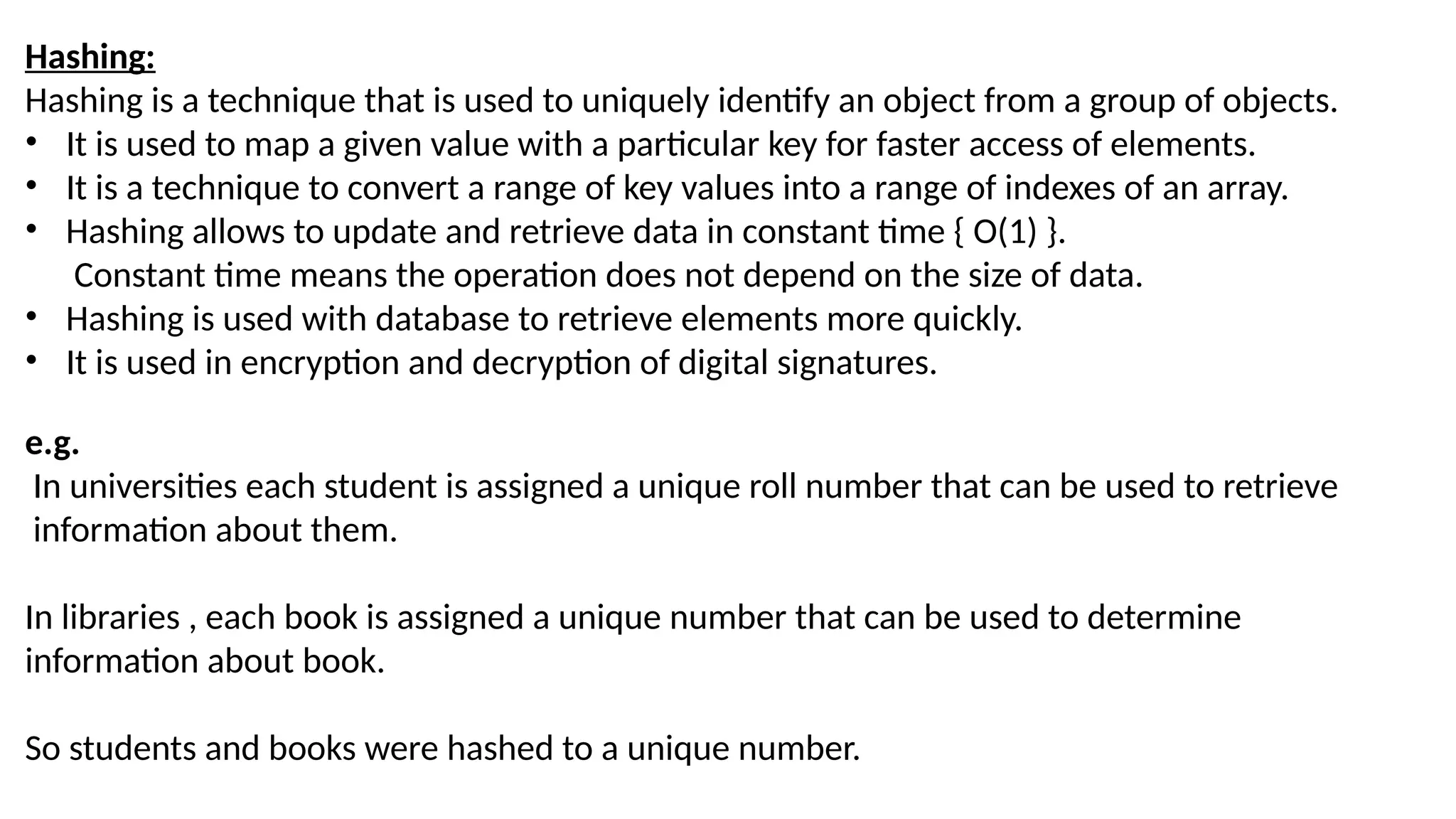
Hashing: Hashing is a technique that is used to uniquely identify an object from a group of objects. • It is used to map a given value with a particular key for faster access of elements. • It is a technique to convert a range of key values into a range of indexes of an array. • Hashing allows to update and retrieve data in constant time { O(1) }. Constant time means the operation does not depend on the size of data. • Hashing is used with database to retrieve elements more quickly. • It is used in encryption and decryption of digital signatures. e.g. In universities each student is assigned a unique roll number that can be used to retrieve information about them. In libraries , each book is assigned a unique number that can be used to determine information about book. So students and books were hashed to a unique number.

In hashing large keys are converted into small keys by using hash function. The values are then stored in a data structure called hash table. The idea of hashing is to describe entries (key/value) uniformly across an array. Each element is assigned a key (converted key). By using that key we can access the element in O(1) time. Using the key , the algorithm (hash function) computes an index that finds where an entry can be found or inserted. Hashing is a technique to convert a range of key values into a range of indexes of array. Item are in the (key, value) format.

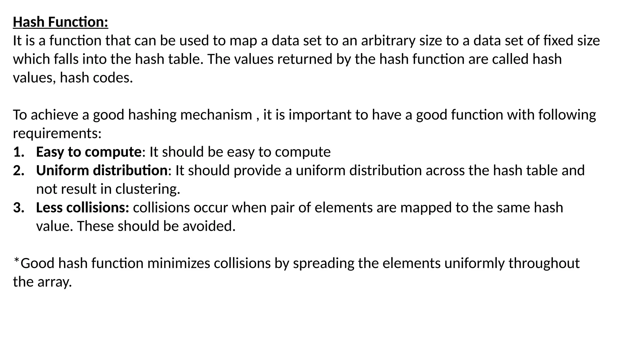
Key-1 Key-2 Key-3 Hash function Index Value 0 Value-1 1 Value-2 2 Value-3 3 Value-4 S. No. Key Hash Array Index 1 1 1%20=1 1 2 2 2%20=2 2 3 42 42%20=2 2 4 4 4%20=4 4 5 12 12%20=12 12 6 14 14%20=14 14 7 17 17%20=17 17 (1,20) (2,70) (42,80) (4,25) (12,44) (14,32) (17,11)

Hash Function: It is a function that can be used to map a data set to an arbitrary size to a data set of fixed size which falls into the hash table. The values returned by the hash function are called hash values, hash codes. To achieve a good hashing mechanism , it is important to have a good function with following requirements: 1. Easy to compute: It should be easy to compute 2. Uniform distribution: It should provide a uniform distribution across the hash table and not result in clustering. 3. Less collisions: collisions occur when pair of elements are mapped to the same hash value. These should be avoided. *Good hash function minimizes collisions by spreading the elements uniformly throughout the array.

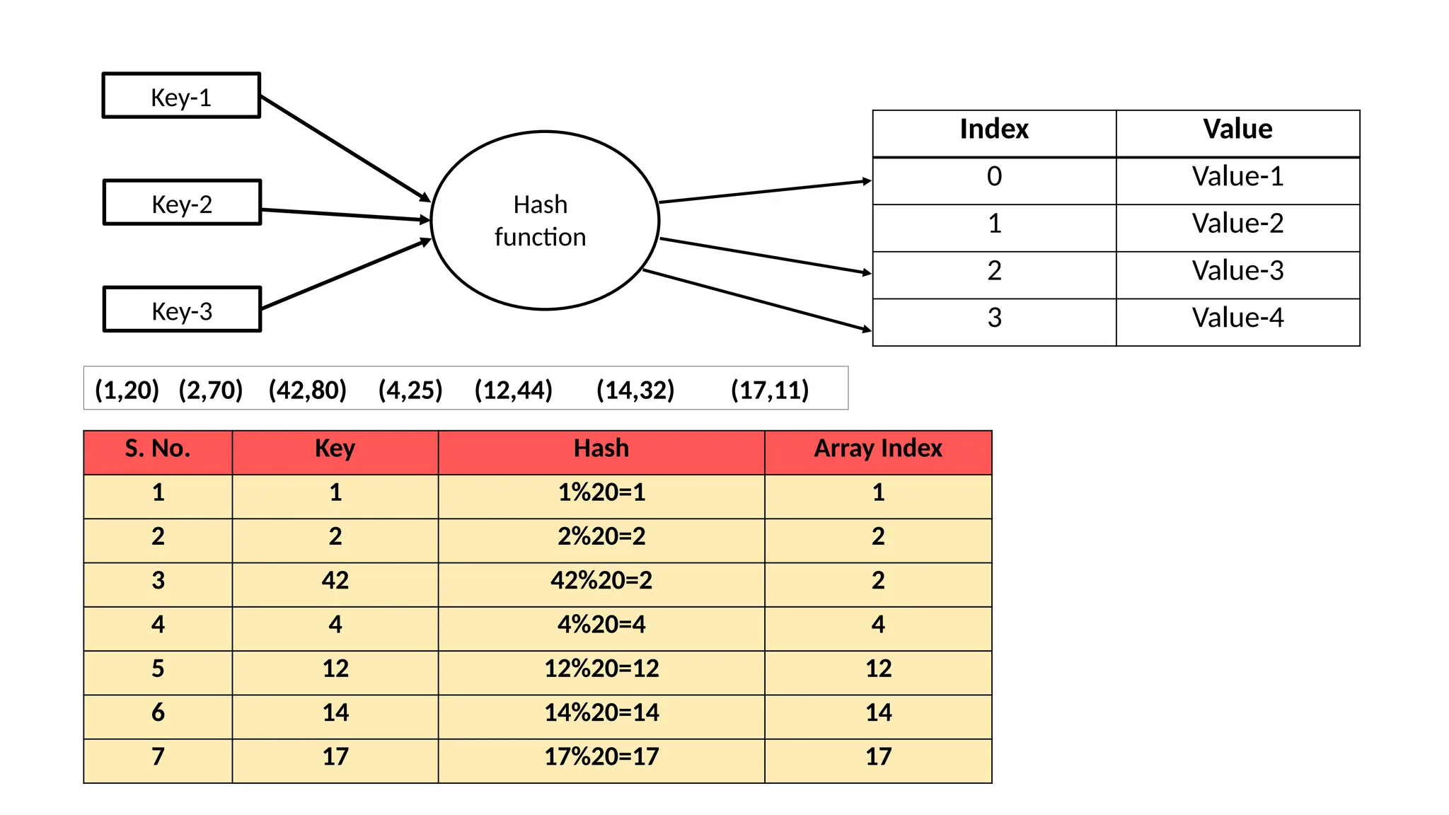
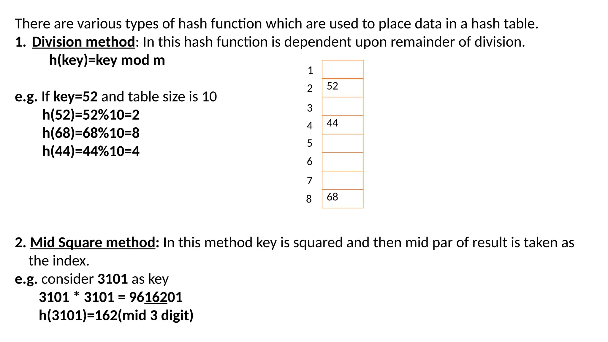
There are various types of hash function which are used to place data in a hash table. 1. Division method: In this hash function is dependent upon remainder of division. h(key)=key mod m e.g. If key=52 and table size is 10 h(52)=52%10=2 h(68)=68%10=8 h(44)=44%10=4 2. Mid Square method: In this method key is squared and then mid par of result is taken as the index. e.g. consider 3101 as key 3101 * 3101 = 9616201 h(3101)=162(mid 3 digit) 52 44 68 1 2 3 4 5 6 7 8

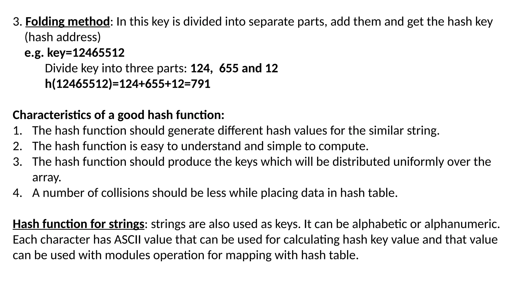
3. Folding method: In this key is divided into separate parts, add them and get the hash key (hash address) e.g. key=12465512 Divide key into three parts: 124, 655 and 12 h(12465512)=124+655+12=791 Characteristics of a good hash function: 1. The hash function should generate different hash values for the similar string. 2. The hash function is easy to understand and simple to compute. 3. The hash function should produce the keys which will be distributed uniformly over the array. 4. A number of collisions should be less while placing data in hash table. Hash function for strings: strings are also used as keys. It can be alphabetic or alphanumeric. Each character has ASCII value that can be used for calculating hash key value and that value can be used with modules operation for mapping with hash table.

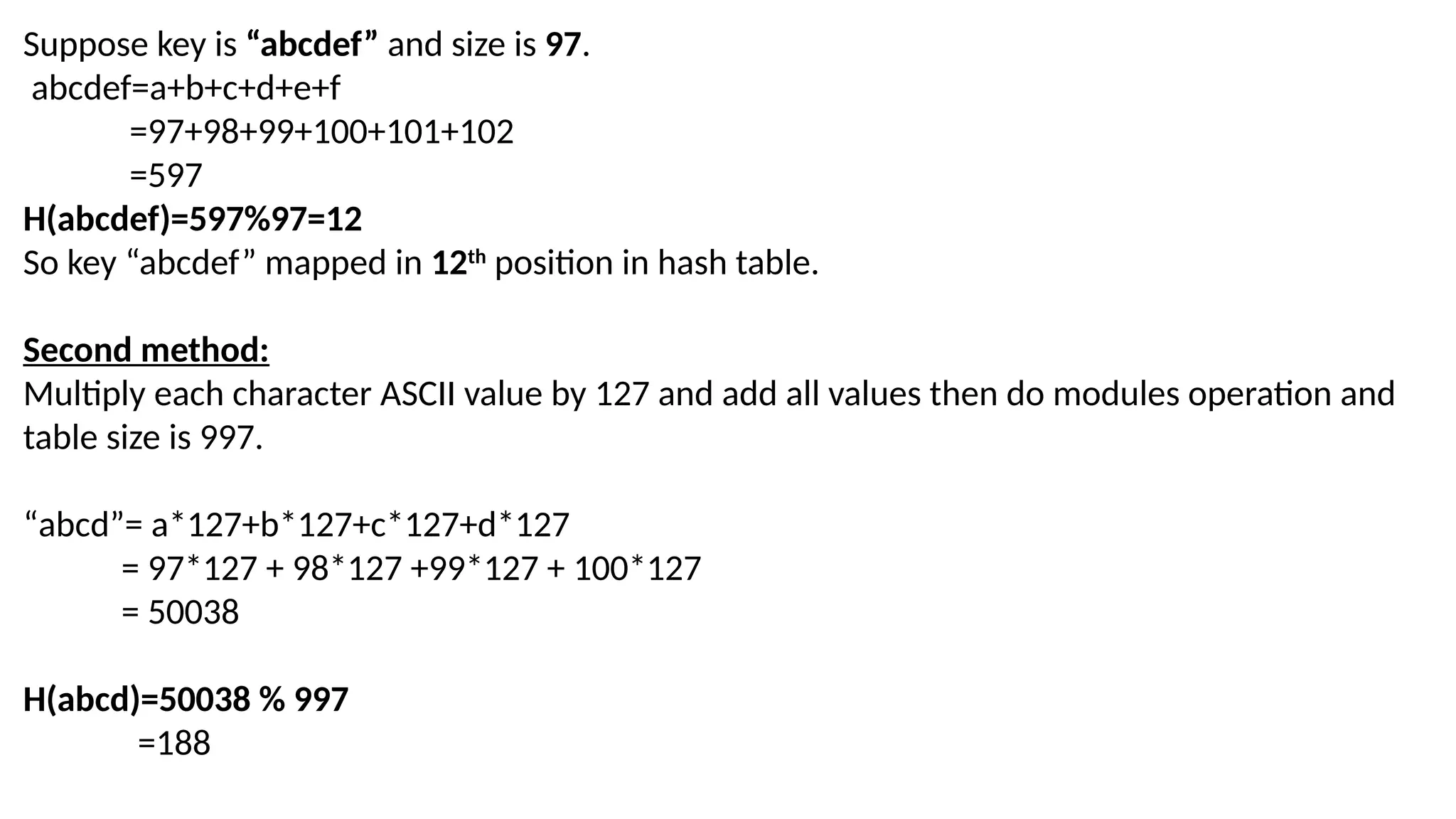
Suppose key is “abcdef” and size is 97. abcdef=a+b+c+d+e+f =97+98+99+100+101+102 =597 H(abcdef)=597%97=12 So key “abcdef” mapped in 12th position in hash table. Second method: Multiply each character ASCII value by 127 and add all values then do modules operation and table size is 997. “abcd”= a*127+b*127+c*127+d*127 = 97*127 + 98*127 +99*127 + 100*127 = 50038 H(abcd)=50038 % 997 =188

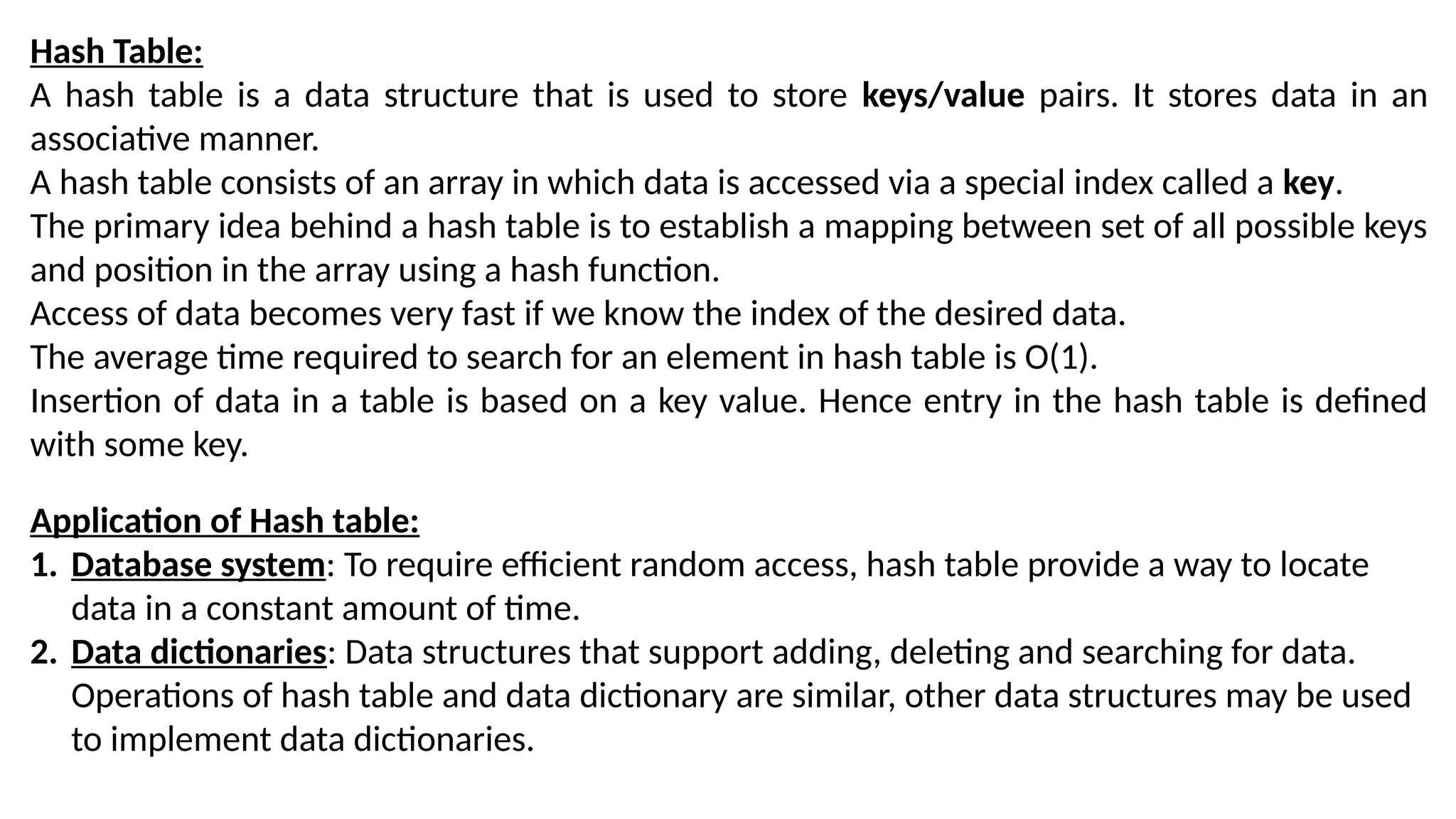
Hash Table: A hash table is a data structure that is used to store keys/value pairs. It stores data in an associative manner. A hash table consists of an array in which data is accessed via a special index called a key. The primary idea behind a hash table is to establish a mapping between set of all possible keys and position in the array using a hash function. Access of data becomes very fast if we know the index of the desired data. The average time required to search for an element in hash table is O(1). Insertion of data in a table is based on a key value. Hence entry in the hash table is defined with some key. Application of Hash table: 1. Database system: To require efficient random access, hash table provide a way to locate data in a constant amount of time. 2. Data dictionaries: Data structures that support adding, deleting and searching for data. Operations of hash table and data dictionary are similar, other data structures may be used to implement data dictionaries.

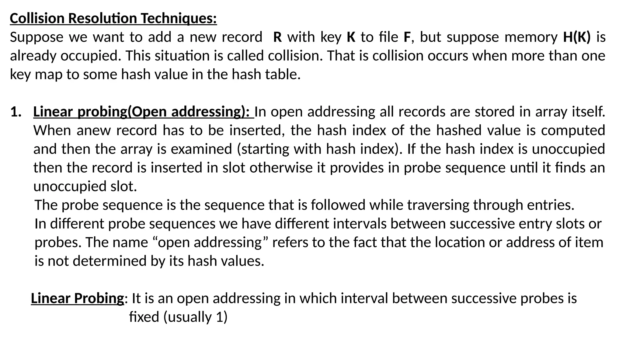
Collision Resolution Techniques: Suppose we want to add a new record R with key K to file F, but suppose memory H(K) is already occupied. This situation is called collision. That is collision occurs when more than one key map to some hash value in the hash table. 1. Linear probing(Open addressing): In open addressing all records are stored in array itself. When anew record has to be inserted, the hash index of the hashed value is computed and then the array is examined (starting with hash index). If the hash index is unoccupied then the record is inserted in slot otherwise it provides in probe sequence until it finds an unoccupied slot. The probe sequence is the sequence that is followed while traversing through entries. In different probe sequences we have different intervals between successive entry slots or probes. The name “open addressing” refers to the fact that the location or address of item is not determined by its hash values. Linear Probing: It is an open addressing in which interval between successive probes is fixed (usually 1)

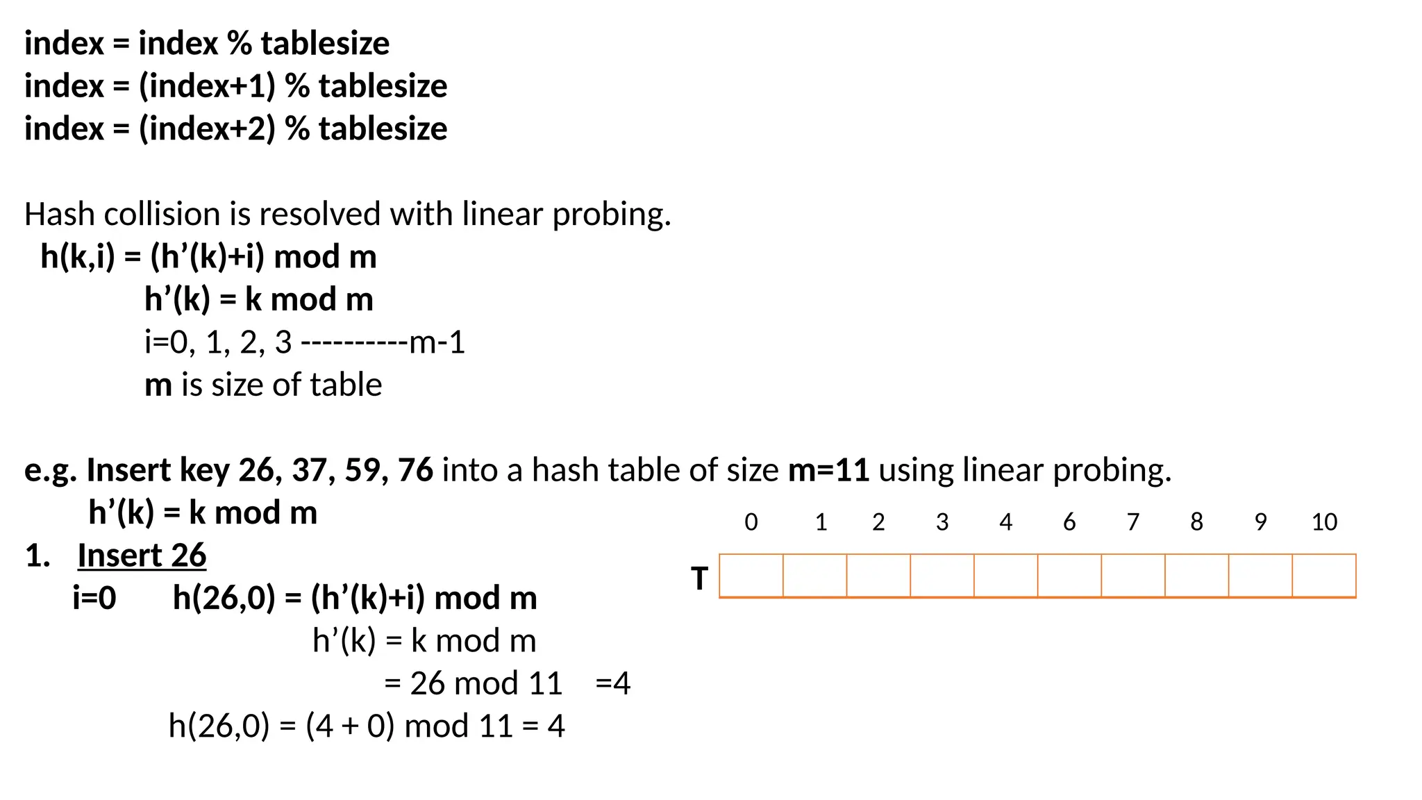
index = index % tablesize index = (index+1) % tablesize index = (index+2) % tablesize Hash collision is resolved with linear probing. h(k,i) = (h’(k)+i) mod m h’(k) = k mod m i=0, 1, 2, 3 ----------m-1 m is size of table e.g. Insert key 26, 37, 59, 76 into a hash table of size m=11 using linear probing. h’(k) = k mod m 1. Insert 26 i=0 h(26,0) = (h’(k)+i) mod m h’(k) = k mod m = 26 mod 11 =4 h(26,0) = (4 + 0) mod 11 = 4 T 0 1 2 3 4 6 7 8 9 10

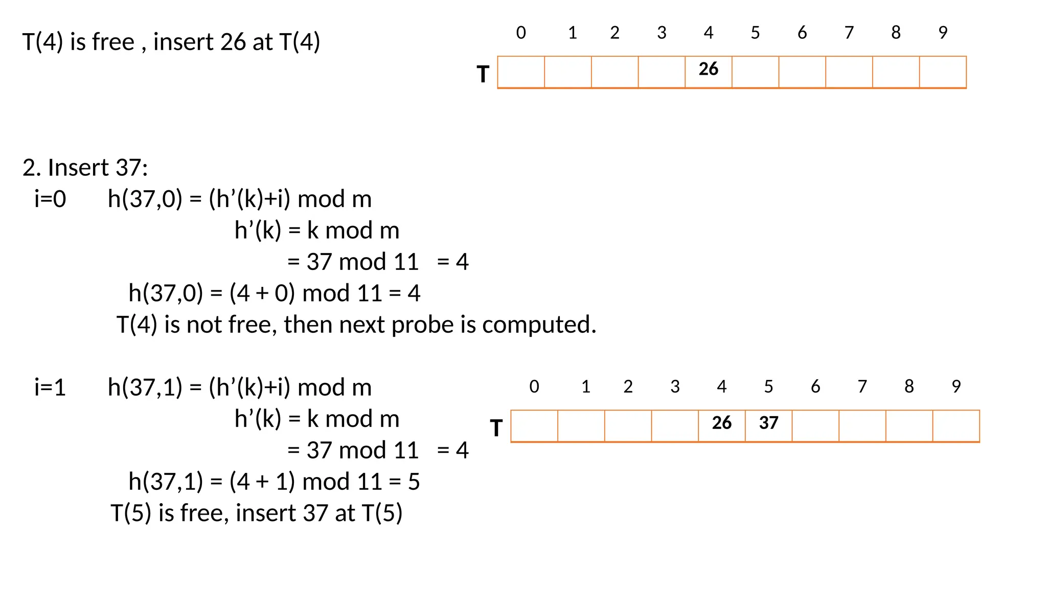
T(4) is free , insert 26 at T(4) 2. Insert 37: i=0 h(37,0) = (h’(k)+i) mod m h’(k) = k mod m = 37 mod 11 = 4 h(37,0) = (4 + 0) mod 11 = 4 T(4) is not free, then next probe is computed. i=1 h(37,1) = (h’(k)+i) mod m h’(k) = k mod m = 37 mod 11 = 4 h(37,1) = (4 + 1) mod 11 = 5 T(5) is free, insert 37 at T(5) 26 T 0 1 2 3 4 5 6 7 8 9 26 37 T 0 1 2 3 4 5 6 7 8 9

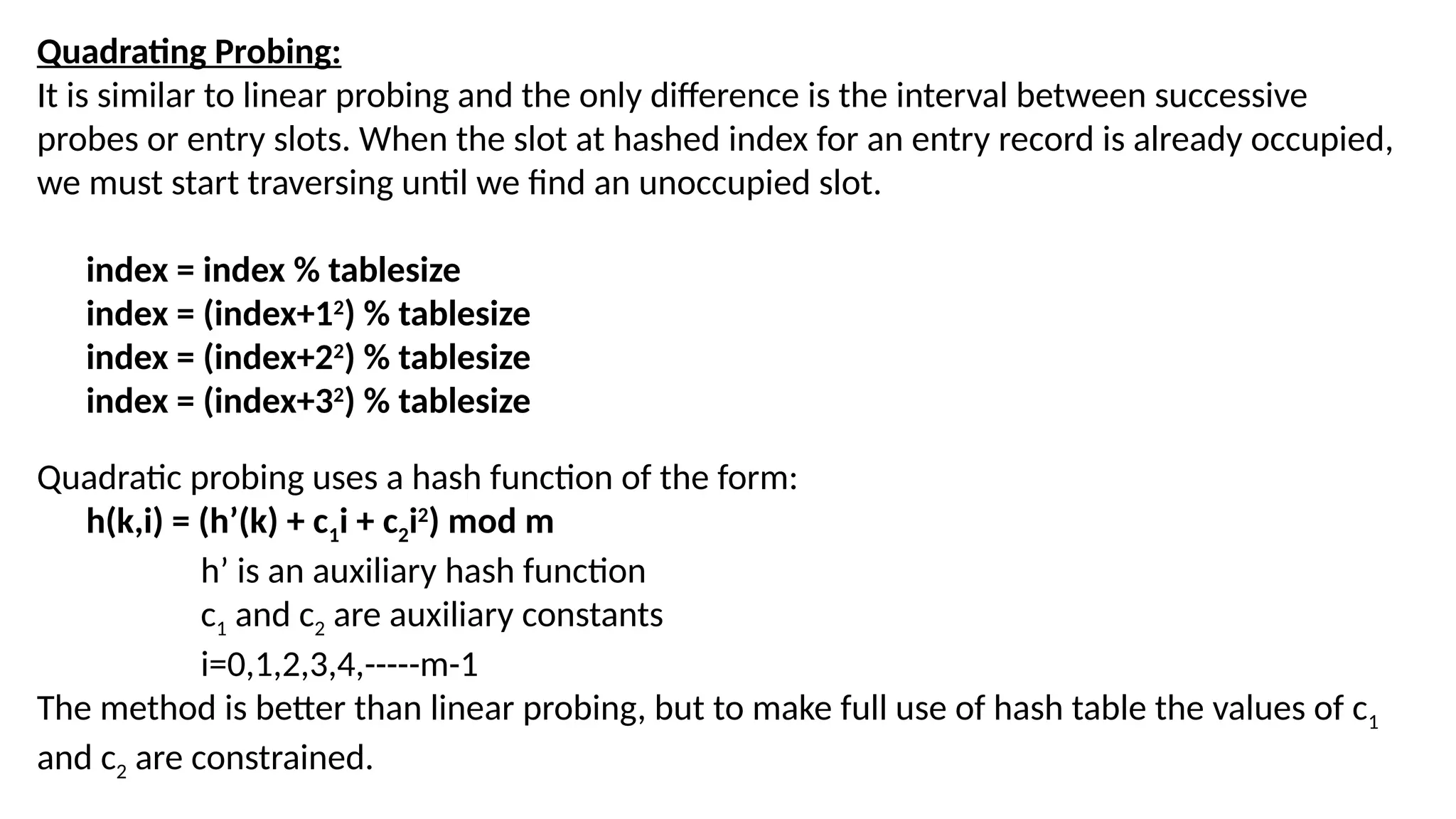
Quadrating Probing: It is similar to linear probing and the only difference is the interval between successive probes or entry slots. When the slot at hashed index for an entry record is already occupied, we must start traversing until we find an unoccupied slot. index = index % tablesize index = (index+12 ) % tablesize index = (index+22 ) % tablesize index = (index+32 ) % tablesize Quadratic probing uses a hash function of the form: h(k,i) = (h’(k) + c1i + c2i2 ) mod m h’ is an auxiliary hash function c1 and c2 are auxiliary constants i=0,1,2,3,4,-----m-1 The method is better than linear probing, but to make full use of hash table the values of c1 and c2 are constrained.

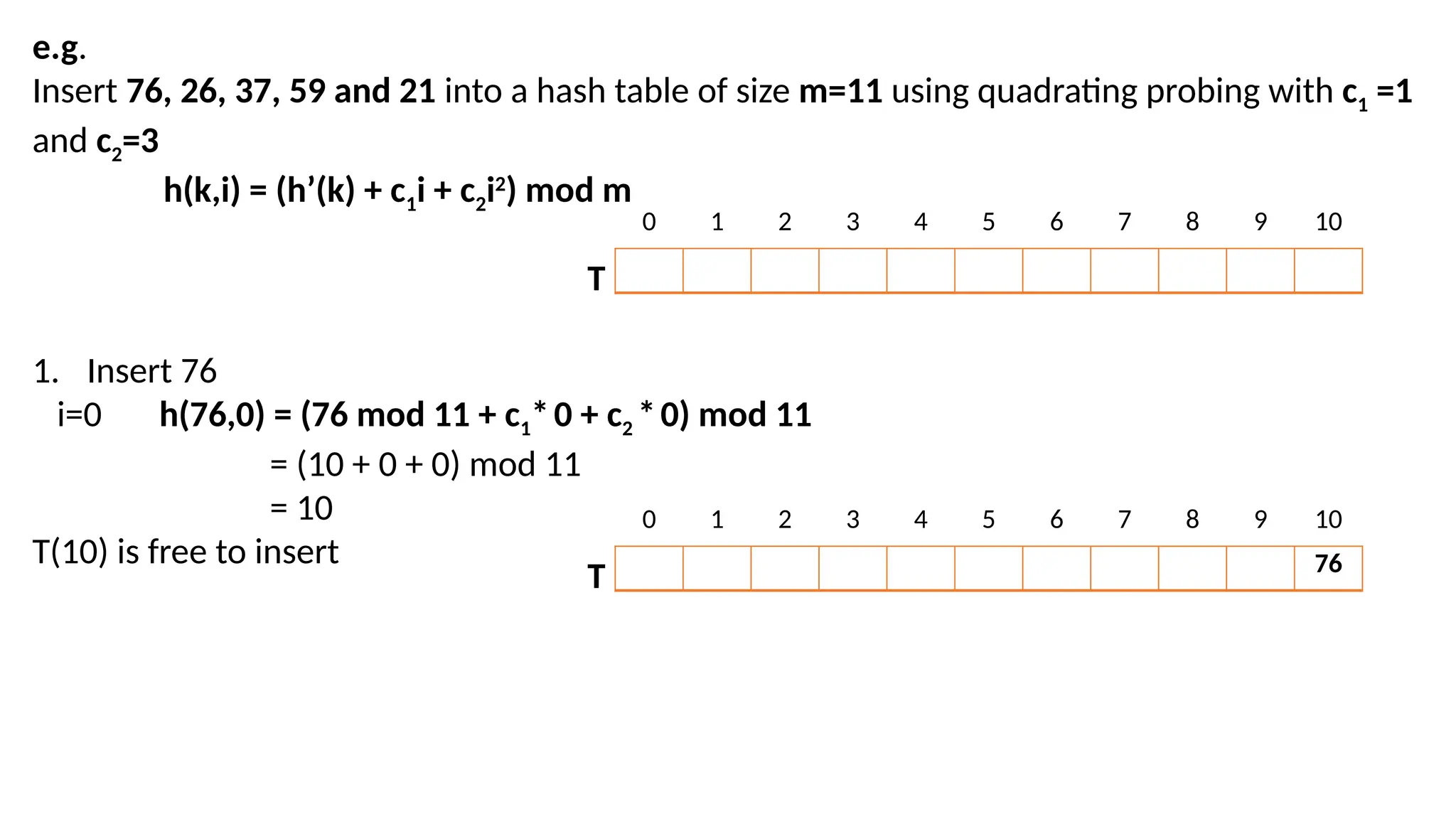
e.g. Insert 76, 26, 37, 59 and 21 into a hash table of size m=11 using quadrating probing with c1 =1 and c2=3 h(k,i) = (h’(k) + c1i + c2i2 ) mod m 1. Insert 76 i=0 h(76,0) = (76 mod 11 + c1*0 + c2 *0) mod 11 = (10 + 0 + 0) mod 11 = 10 T(10) is free to insert 0 1 2 3 4 5 6 7 8 9 10 T 76 0 1 2 3 4 5 6 7 8 9 10 T

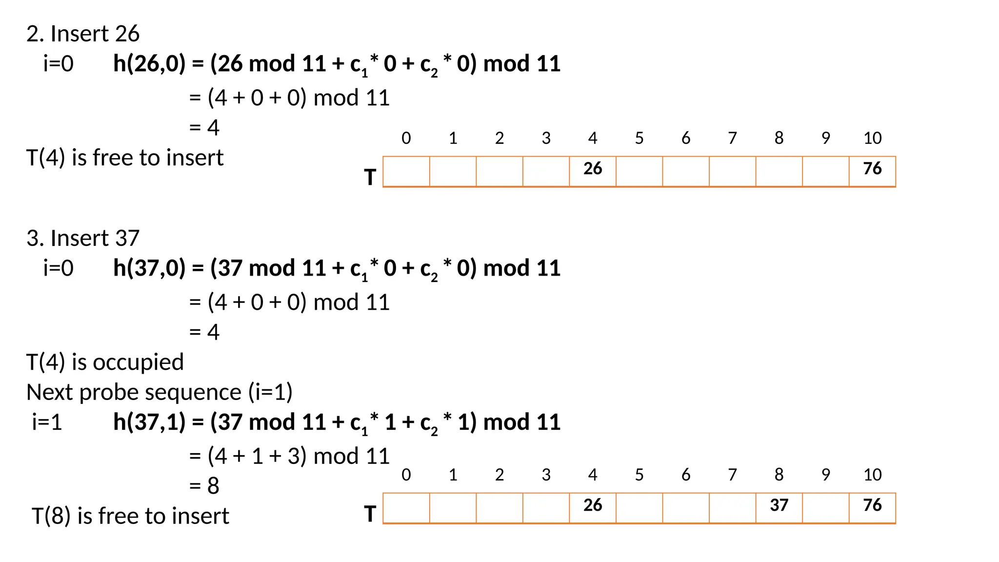
2. Insert 26 i=0 h(26,0) = (26 mod 11 + c1*0 + c2 *0) mod 11 = (4 + 0 + 0) mod 11 = 4 T(4) is free to insert 26 76 0 1 2 3 4 5 6 7 8 9 10 T 3. Insert 37 i=0 h(37,0) = (37 mod 11 + c1*0 + c2 *0) mod 11 = (4 + 0 + 0) mod 11 = 4 T(4) is occupied Next probe sequence (i=1) i=1 h(37,1) = (37 mod 11 + c1*1 + c2 *1) mod 11 = (4 + 1 + 3) mod 11 = 8 T(8) is free to insert 26 37 76 0 1 2 3 4 5 6 7 8 9 10 T

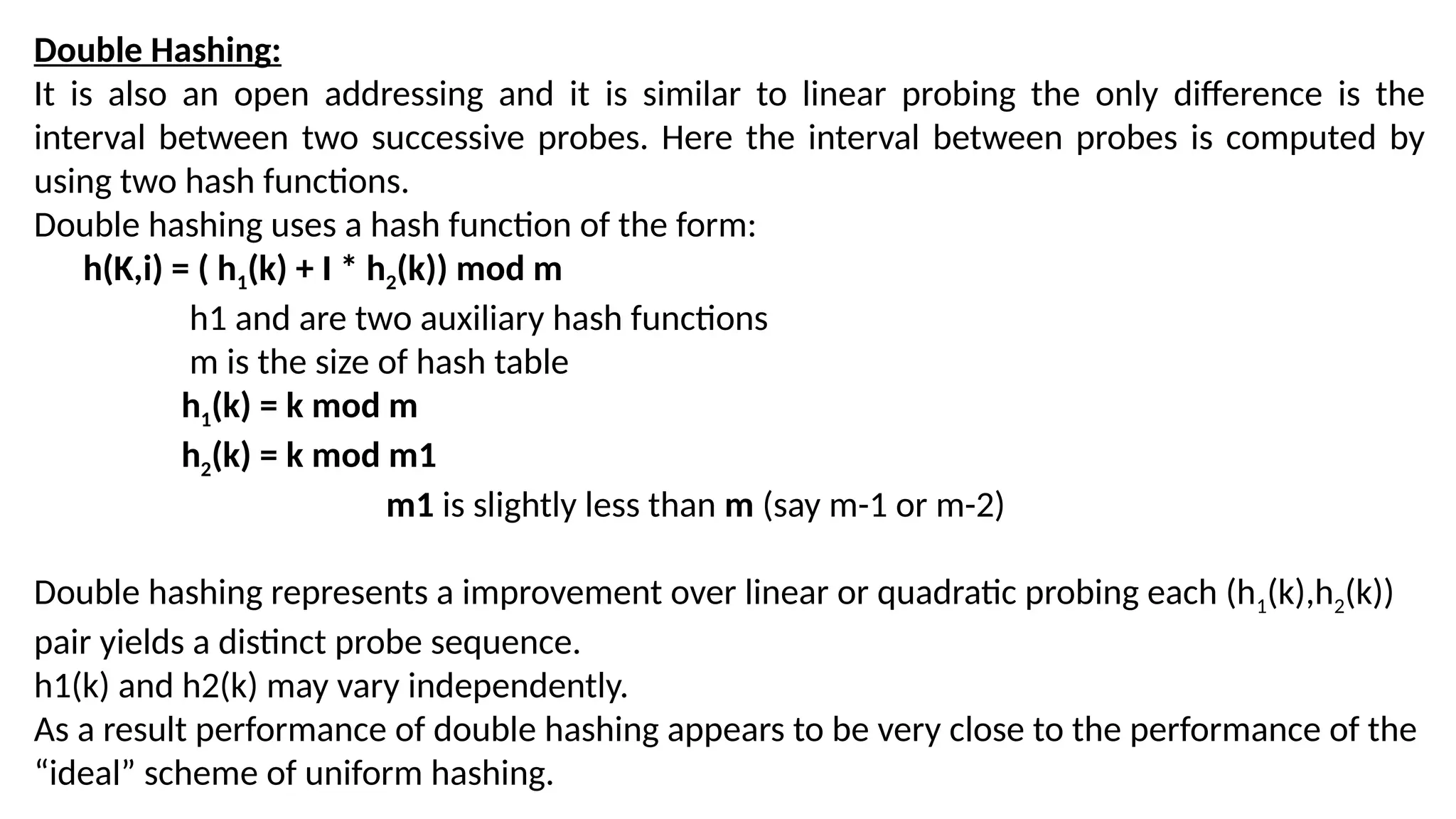
Double Hashing: It is also an open addressing and it is similar to linear probing the only difference is the interval between two successive probes. Here the interval between probes is computed by using two hash functions. Double hashing uses a hash function of the form: h(K,i) = ( h1(k) + I * h2(k)) mod m h1 and are two auxiliary hash functions m is the size of hash table h1(k) = k mod m h2(k) = k mod m1 m1 is slightly less than m (say m-1 or m-2) Double hashing represents a improvement over linear or quadratic probing each (h1(k),h2(k)) pair yields a distinct probe sequence. h1(k) and h2(k) may vary independently. As a result performance of double hashing appears to be very close to the performance of the “ideal” scheme of uniform hashing.

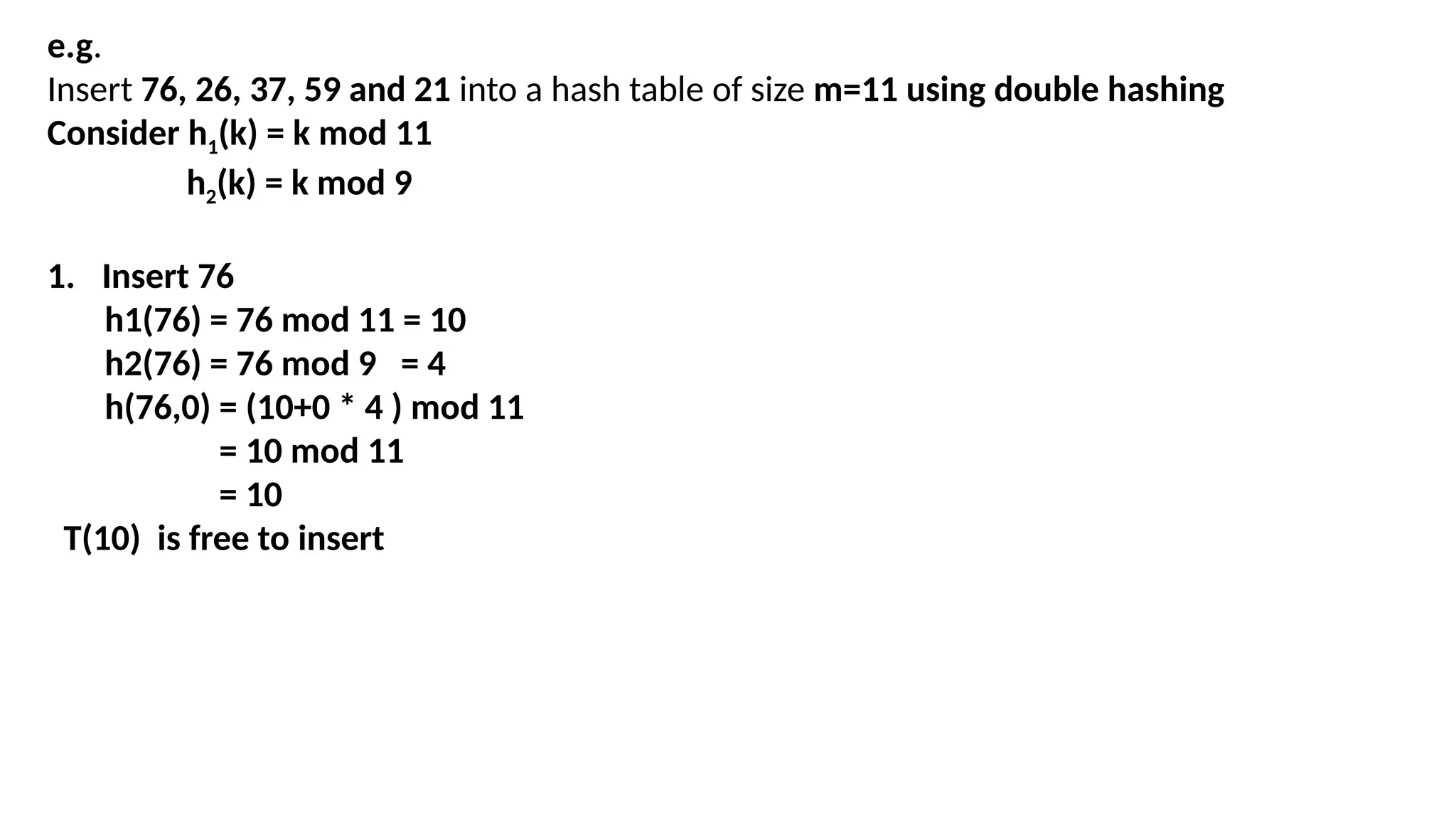
e.g. Insert 76, 26, 37, 59 and 21 into a hash table of size m=11 using double hashing Consider h1(k) = k mod 11 h2(k) = k mod 9 1. Insert 76 h1(76) = 76 mod 11 = 10 h2(76) = 76 mod 9 = 4 h(76,0) = (10+0 * 4 ) mod 11 = 10 mod 11 = 10 T(10) is free to insert

Data structure Graph PPT ( BFS & DFS ) NOTES

More Related Content

Similar to Data structure Graph PPT ( BFS & DFS ) NOTES

Recently uploaded

Data structure Graph PPT ( BFS & DFS ) NOTES