Data structure and algorithms unit 1 pdf SRM

18CSC201J DATA STRUCTURES AND ALGORITHMS UNIT 1 Prepared by Dr. Pretty Diana Cyril Dr. S. Thanga Revathi Dr. Mary Subaja Christo Dr. K. Kalai selvi R Lavanya

Topics to be covered S1 : Introduction – Basic Terminology - Data Structures S2 : Data Structure Operations - ADT S3 : Algorithms – Searching Techniques – Complexity – Time, Space Matrix S4 : Algorithms – Sorting - Complexity – Time, Space Matrix S5 : Mathematical notations – Asymptotic notations – Big O, Omega S6 : Asymptotic notations – Theta – Mathematical functions S7 : Data Structures and its Types - Linear and Non Linear Data Structures S8 : 1D, 2D Array Initialization using Pointers - 1D, 2D Array Accessing using Pointers S9 : Declaring Structure and accessing – Declaring Arrays of Structures and accessing

INTRODUCTION BASIC TERMINOLOGY

Introduction • Data Structure can be defined as the group of data elements which provides an efficient way of storing and organizing data in the computer so that it can be used efficiently. • Some examples of Data Structures are arrays, Linked List, Stack, Queue, etc. • Data Structures are widely used in almost every aspect of Computer Science i.e. Operating System, Compiler Design, Artificial intelligence, Graphics and many more.

Basic Terminology • Data are values or sets of values • A data item refers to a single unit of values. Data items are divided into subitems are called group items. oFor example, an employee’s name may be divided into three subitems first name, middle name and last name but the social security number would treated as a single name. • Collections of data are organized into a hierarchy of fields, records and files.

Basic Terminology (Cont..) • Record can be defined as the collection of various data items. oFor example, if we talk about the student entity, then its name, address, course and marks can be grouped together to form the record for the student. • Record is classified according to length. A file can have fixed length records or variable length records. • In fixed length records, all the records contain the same data items with the same amount of space assigned to each data items. • In variable length records, file records may contain different lengths. Variable length records have a minimum and a maximum length. oFor example, student records have variable length, since different students take different numbers of courses

Basic Terminology (Cont..) • A File is a collection of various records of one type of entity. oFor example, if there are 60 employees in the class, then there will be 20 records in the related file where each record contains the data about each employee. • An entity represents the class of certain objects. It contains various attributes. Each attribute represents the particular property of that entity. oFor example, consider an employee of an organization: Attributes: Name Age Sex Social Security Number Values: JOHN 34 M 134-24-5533 • Field is a single elementary unit of information representing the attribute of an entity.

Basic Terminology – Example • A professor keeps a class list containing the following data for each student: Name, Major, Student Number, Test Scores, Final Grades a) State the entities, attributes and entity set of the list. b) Describe the field values, records and file. c) Which attribute can serve as primary keys for the list? a) Each student is an entity, and the collection of students is the entity set. The properties, name, major, and so on. of the students are the attributes. b) The field values are the values assigned to the attributes, i. e., the actual names, test scores, and so on. The field values for each student constitute a record, and the collection of all the student records is the file. c) Either Name or Student Number can serve as a primary key, since each uniquely determines the student’s record. Normally the professor uses Name as the primary key, but the registrar may use students Number.

Data Structures • Data Structure can be defined as the group of data elements which provides an efficient way of storing and organizing data in the computer so that it can be used efficiently. • Data Structures are the main part of many computer science algorithms as they enable the programmers to handle the data in an efficient way. • It plays a vital role in enhancing the performance of a software or a program as the main function of the software is to store and retrieve the user's data as fast as possible.

Classification of Data Structures

Primitive & Non-Primitive of Data Structures • Primitive data structures are the fundamental data types which are supported by a programming language. • Some basic data types are integer, real(float), character, and Boolean. • Non-primitive data structures are data structures which are created using primitive data structures. • Examples of such data structures include linked lists, stacks, trees, and graphs. • Non-primitive data structures can further be classified into two categories: linear and non-linear data structures.

Linear Data Structures • If the elements of a data structure are stored in a linear or sequential order, then it is a linear data structure. • Examples include arrays, linked lists, stacks, and queues. • Linear data structures can be represented in memory in two different ways. • One way is to have a linear relationship between elements by means of sequential memory locations. • The other way is to have a linear relationship between elements by means of links.

Non Linear Data Structures • If the elements of a data structure are not stored in a sequential order, then it is a non-linear data structure. • The relationship of adjacency is not maintained between elements of a non-linear data structure. • Examples include trees and graphs.

Review Questions • A hospital maintains a patient file in which each record contains the following data: Name, Admission date, Social security number, Room, Bed number, Doctor a) Which items can serve as primary keys? b) Which pair of items can serve as a primary key? c) Which items can be group items? • Which of the following data items may lead to variable length records when included as items in the record: (a) age, (b) sex, (c) name of spouse, (d) names of children, (e) education, (f) previous employers

Data Structure Operations • The data in the data structures are processed by certain operations. oTraversing oSearching oInserting oUpdating oDeleting oSorting oMerging

Data Structure Operations (Cont..) • Traversing - Visiting each record so that items in the records can be accessed. • Searching - Finding the location of the record with a given key or value or finding all records which satisfy given conditions. • Inserting - Adding a new record to the data structure. • Updating – Change the content of some elements of the record. • Deleting - Removing records from the data structure. • Sorting - Arranging records in some logical or numerical order. o(Eg: Alphabetic order) • Merging - Combing records from two different sorted files into a single file.

Example • An organization contains a membership file in which each record contains the following data for a given member: Name, Address, Telephone Number, Age, Sex a. Suppose the organization wants to announce a meeting through a mailing. Then one would traverse the file to obtain Name and Address of each member. b. Suppose one wants to find the names of all members living in a particular area. Again traverse and search the file to obtain the data. c. Suppose one wants to obtain Address of a specific Person. Then one would search the file for the record containing Name. d. Suppose a member dies. Then one would delete his or her record from the file.

Example e. Suppose a new person joins the organization. Then one would insert a record into the file f. Suppose a member has shifted to a new residence his/her address and telephone number need to be changed. Given the name of the member, one would first need to search for the record in the file. Then perform the update operation, i.e. change some items in the record with the new data. g. Suppose one wants to find the number of members whose age is 65 or above. Again one would traverse the file, counting such members.

Abstract Data Types • An Abstract Data type (ADT) is a type for objects whose behavior is defined by a set of value and a set of operations. • ADT refers to a set of data values and associated operations that are specified accurately, independent of any particular implementation. • The ADT consists of a set of definitions that allow us to use the functions while hiding the implementation. • Abstract in the context of data structures means everything except the detailed specifications or implementation. • Data type of a variable is the set of values that the variable can take. • Examples: Stacks, Queues, Linked List ADT = Type + Function Names + Behaviour of each function

ADT Operations • While modeling the problems the necessary details are separated out from the unnecessary details. This process of modeling the problem is called abstraction. • The model defines an abstract view to the problem. It focuses only on problem related stuff and that you try to define properties of the problem. • These properties include oThe data which are affected. oThe operations which are identified.

ADT Operations ( Cont..) • Abstract data type operations are oCreate - Create the data structure. oDisplay - Displaying all the elements stored in the data structure. oInsert - Elements can be inserted at any desired position. oDelete - Desired element can be deleted from the data structure. oModify - Any desired element can be deleted/modified from the data structure.

Abstract Data Types Model • The ADT model has two different parts functions (public and private) and data structures. • Both are contained within the ADT model itself, and do not come within the scope of the application program. • Data structures are available to all of the ADT’s functions as required, and a function may call any other function to accomplish its task. • Data structures and functions are within the scope of each other.

Abstract Data Types Model (Cont..) • Data are entered, accessed, modified and deleted through the external application programming interface. • For each ADT operation, there is an algorithm that performs its specific task. • The operation name and parameters are available to the application, and they provide only an interface to the application. • When a list is controlled entirely by the program, it is implemented using simple structure.

Review Questions • ______ are used to manipulate the data contained in various data structures. • In ______, the elements of a data structure are stored sequentially. • ______ of a variable specifies the set of values that the variable can take. • Abstract means ______. • If the elements of a data structure are stored sequentially, then it is a ______.

ALGORITHMS SEARCHING TECHIQUES

Algorithms • An algorithm is a well defined list of steps for solving a particular problem. • The time and space are two major measures of the efficiency of an algorithm. • The complexity of an algorithm is the function which gives the running time and / or space in terms of input size.

Searching Algorithms • Searching Algorithms are designed to check for an element or retrieve an element from any data structure where it is stored. • Based on the type of search operation, these algorithms are generally classified into two categories: • Linear Search • Binary Search

Linear Search • Linear search is a very basic and simple search algorithm. • In Linear search, we search an element or value in a given array by traversing the array from the starting, till the desired element or value is found or we can establish that the element is not present. • It compares the element to be searched with all the elements present in the array and when the element is matched successfully, it returns the index of the element in the array, else it return -1. • Linear search is applied on unsorted or unordered lists, when there are fewer elements in a list.

Linear Search - Example • Search each record of the file, one at a time, until finding the given value.

Algorithm for Linear Search • In Steps 1 and 2 of the algorithm, we initialize the value of POS and I. • In Step 3, a while loop is executed that would be executed till I is less than N. • In Step 4, a check is made to see if a match is found between the current array element and VAL. • If a match is found, then the position of the array element is printed, else the value of I is incremented to match the next element with VAL. • If all the array elements have been compared with VAL and no match is found, then it means that VAL is not present in the array.

Linear Search - Advantages • When a key element matches the first element in the array, then linear search algorithm is best case because executing time of linear search algorithm is O(n), where n is the number of elements in an array. • The list doesn’t have to sort. Contrary to a binary search, linear searching does not demand a structured list. • Not influenced by the order of insertions and deletions. Since the linear search doesn’t call for the list to be sorted, added elements can be inserted and deleted.

Linear Search - Disadvantages • The drawback of a linear search is the fact that it is time consuming if the size of data is huge. • Every time a vital element matches the last element from the array or an essential element does not match any element Linear search algorithm is the worst case.

Binary Search • Binary Search is used with sorted array or list. In binary search, we follow the following steps: 1) We start by comparing the element to be searched with the element in the middle of the list/array. 2) If we get a match, we return the index of the middle element and terminate the process 3) If the element/number to be searched is greater than the middle element, we pick the elements on the left/right side of the middle element, and move to step 1. 4) If the element/number to be searched is lesser in value than the middle number, then we pick the elements on the right/left side of the middle element, and move to step 1.

Binary Search - Example • Binary Search is useful when there are large number of elements in an array and they are sorted.

Algorithm for Binary Search • In Step 1, we initialize the value of variables, BEG, END, and POS. • In Step 2, a while loop is executed until BEG is less than or equal to END. • In Step 3, the value of MID is calculated. • In Step 4, we check if the array value at MID is equal to VAL. If a match is found, then the value of POS is printed and the algorithm exits. If a match is not found, and if the value of A[MID] is greater than VAL, the value of END is modified, otherwise if A[MID] is greater than VAL, then the value of BEG is altered. • In Step 5, if the value of POS = –1, then VAL is not present in the array and an appropriate message is printed on the screen before the algorithm exits.

Binary Search (Cont..) Advantages • It eliminates half of the list from further searching by using the result of each comparison. • It indicates whether the element being searched is before or after the current position in the list. • This information is used to narrow the search. • For large lists of data, it works significantly better than linear search. Disadvantages • It employs recursive approach which requires more stack space. • Programming binary search algorithm is error prone and difficult. • The interaction of binary search with memory hierarchy i.e. caching is poor.

Difference between Linear & Binary Search Linear Search • Linear Search necessitates the input information to be not sorted • Linear Search needs equality comparisons. • Linear search has complexity C(n)= n/2. • Linear Search needs sequential access. Binary Search • Binary Search necessitates the input information to be sorted. • Binary Search necessitates an ordering contrast. • Binary Search has complexity C(n)= log 2 n. • Binary Search requires random access to this information.

Linear Search – Time & Space Matrix • Time Complexity oWe need to go from the first element to the last so, in the worst case we have to iterate through ‘n’ elements, n being the size of a given array. • Space Complexity oWe don't need any extra space to store anything. oWe just compare the given value with the elements in an array one by one. Space Complexity is O(1) Time Complexity is O(n)

Binary Search – Time & Space Matrix • Time Complexity oWe start from the middle of the array and keep dividing the search area by half. oIn other words, search interval decreases in the power of 2 (2048, 1024, 512, ..). • Space Complexity oWe just need to store three values: `lower_bound`, `upper_bound`, and `middle_position`. Space Complexity is O(1) Time Complexity is O(Log n)

Review Questions • The worst case complexity is ______ when compared with the average case complexity of a binary search algorithm. (a) Equal (b) Greater (c) Less (d) None of these • The complexity of binary search algorithm is (a) O(n) (b) O(n2) (c) O(n log n) (d) O(log n) • Which of the following cases occurs when searching an array using linear search the value to be searched is equal to the first element of the array? (a) Worst case (b) Average case (c) Best case (d) Amortized case • Performance of the linear search algorithm can be improved by using a ______. • The complexity of linear search algorithm is ______.

SORTING • Sorting is a technique to rearrange the elements of a list in ascending or descending order, which can be numerical, lexicographical, or any user- defined order. • Sorting is a process through which the data is arranged in ascending or descending order. Sorting can be classified in two types; 1. Internal Sorts 2. External Sorts

SORTING - INTERNAL SORTS • Internal Sorts:- This method uses only the primary memory during sorting process. All data items are held in main memory and no secondary memory is required for this sorting process. • If all the data that is to be sorted can be accommodated at a time in memory is called internal sorting. There is a limitation for internal sorts; they can only process relatively small lists due to memory constraints. There are 3 types of internal sorts based on the type of process used while sorting. (i) SELECTION :- Ex:- Selection sort algorithm, Heap Sort algorithm (ii) INSERTION :- Ex:- Insertion sort algorithm, Shell Sort algorithm (iii) EXCHANGE :- Ex:- Bubble Sort Algorithm, Quick sort algorithm

SORTING – EXTERNAL SORTS • External Sorts:- Sorting large amount of data requires external or secondary memory. This process uses external memory such as HDD, to store the data which is not fit into the main memory. So, primary memory holds the currently being sorted data only. • All external sorts are based on process of merging. Different parts of data are sorted separately and merged together. Ex:- Merge Sort

INSERTION SORT • Insertion Sort Algorithm sorts array by shifting elements one by one and inserting the right element at the right position • It works similar to the way you sort playing cards in your hands

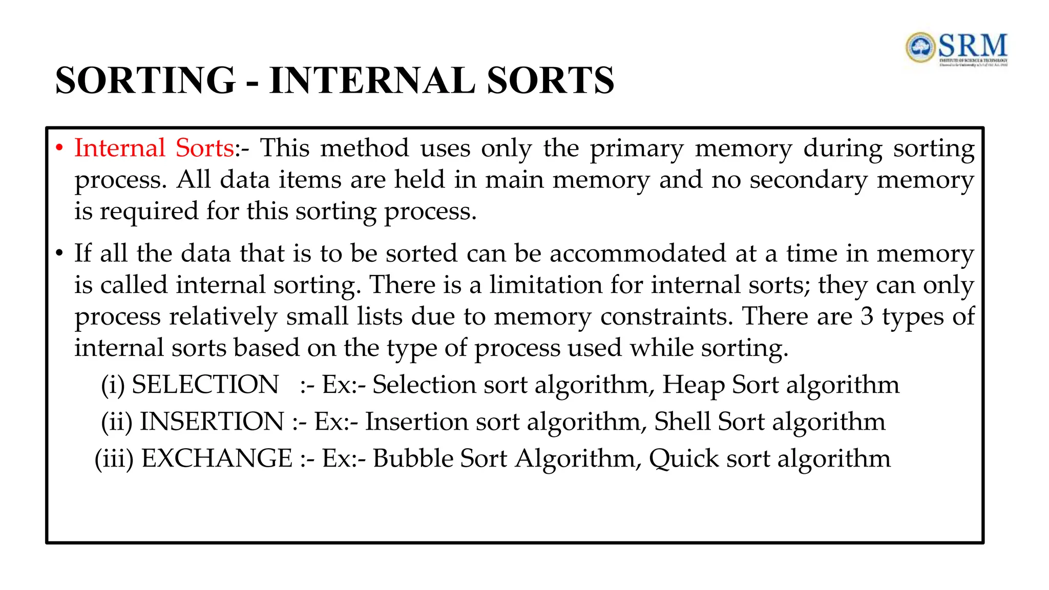
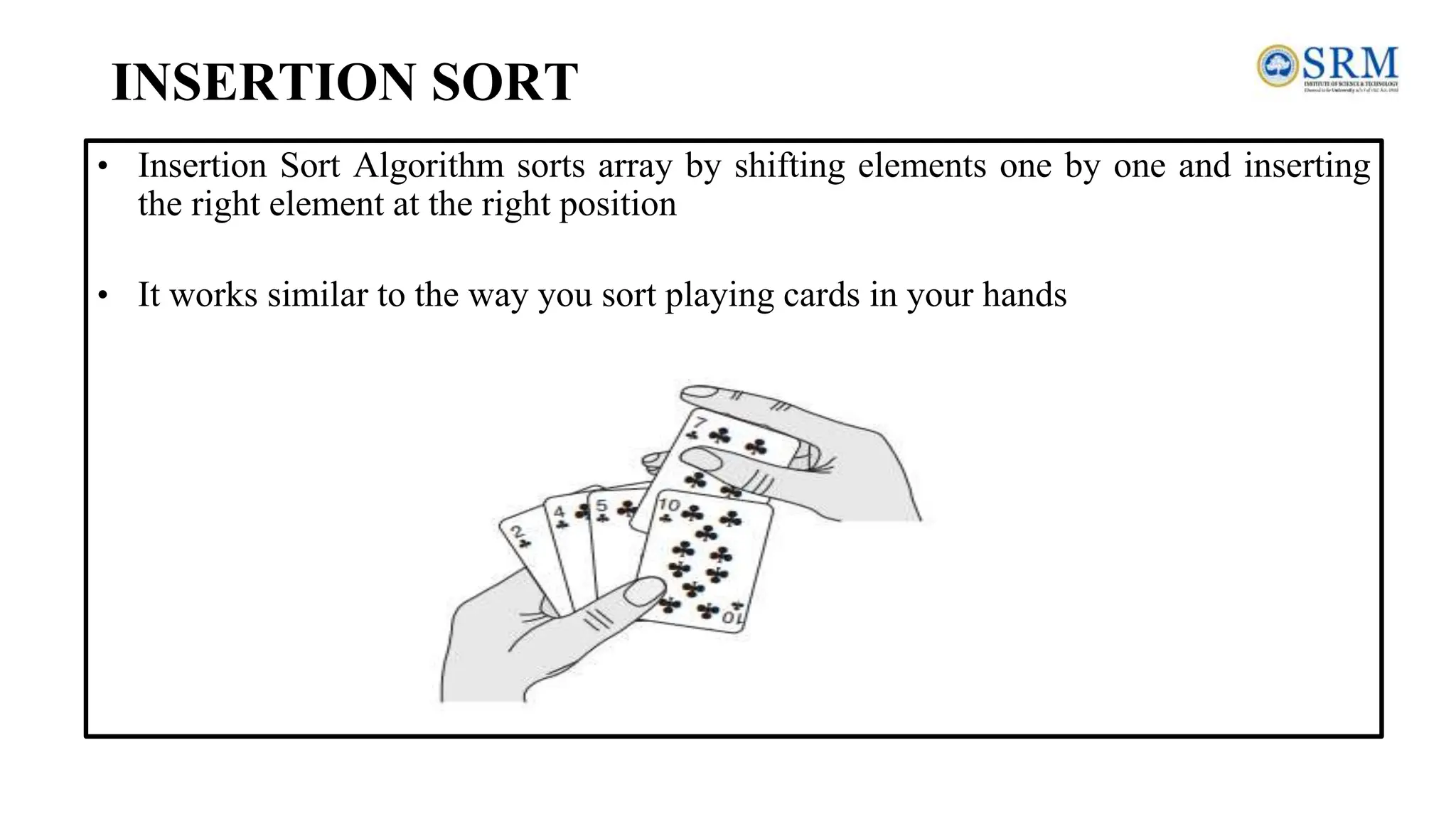
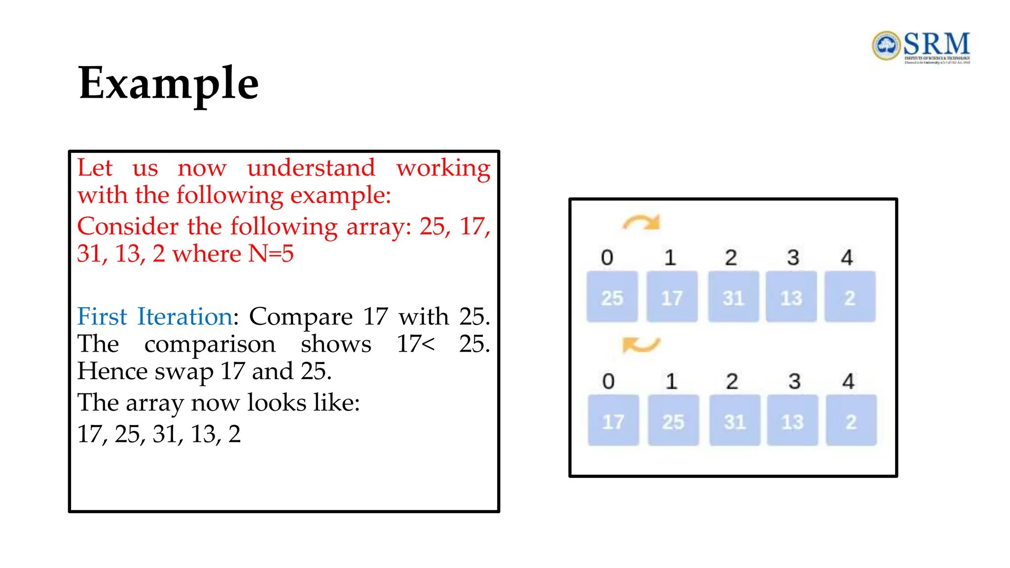
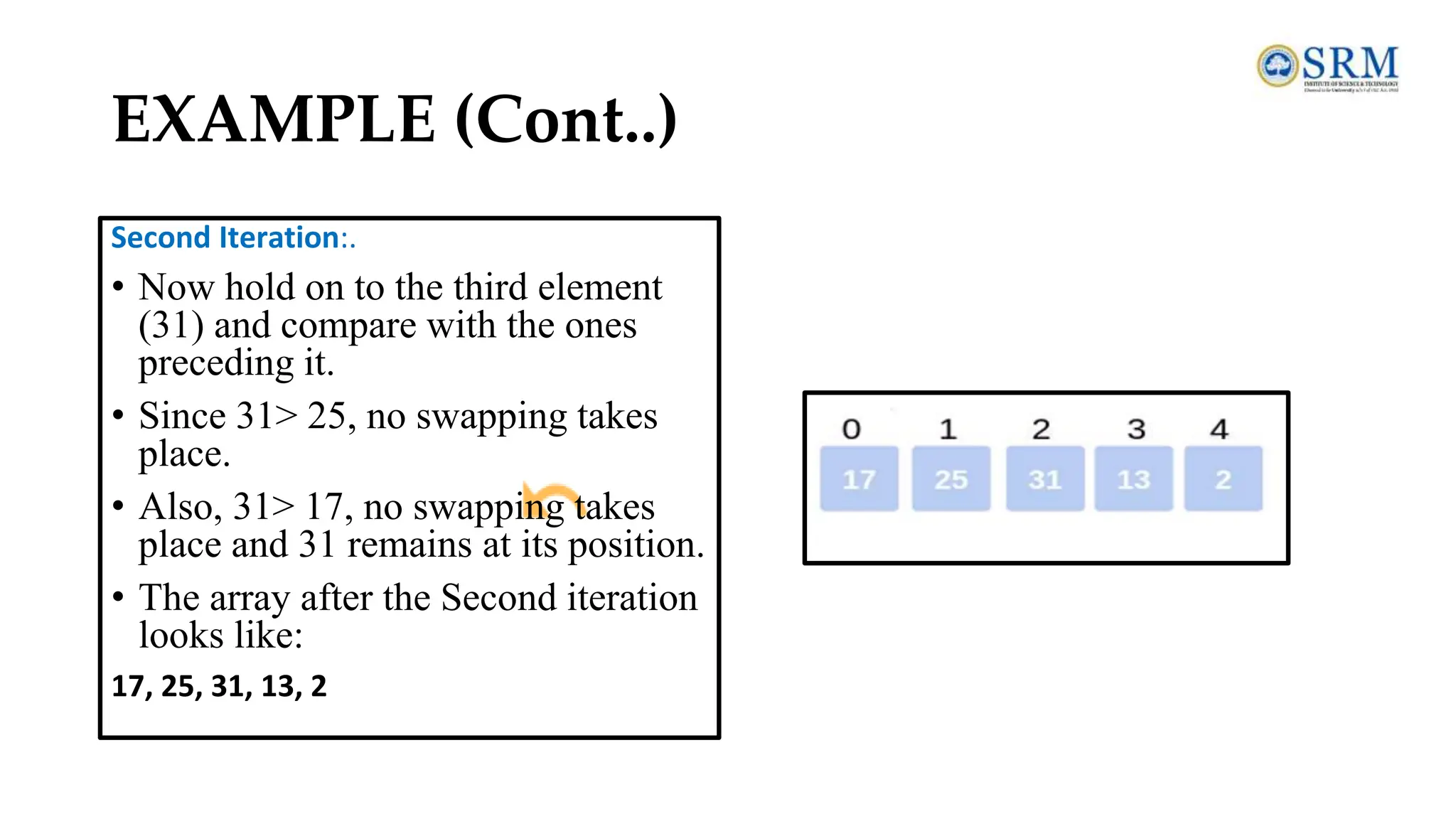
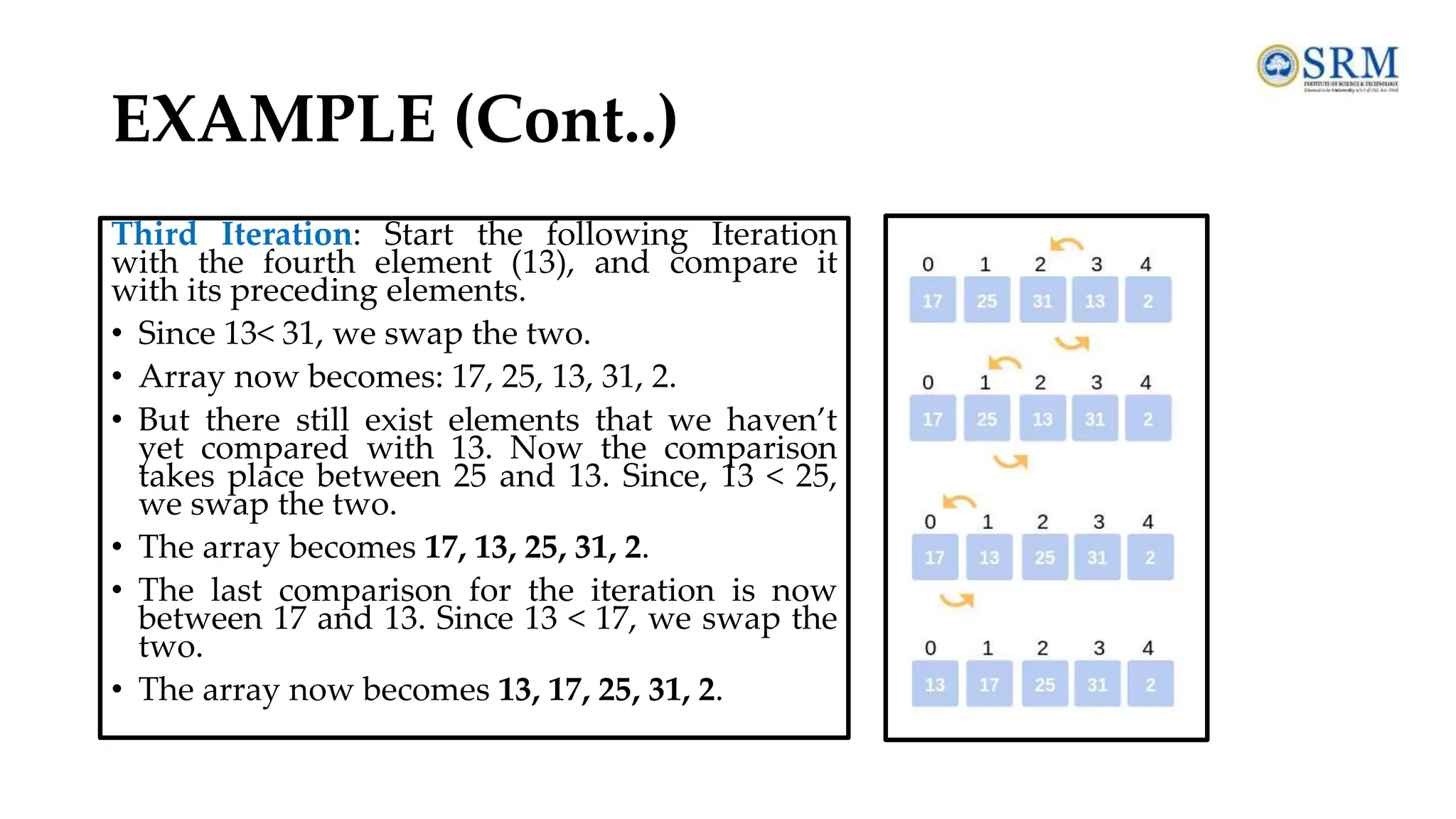
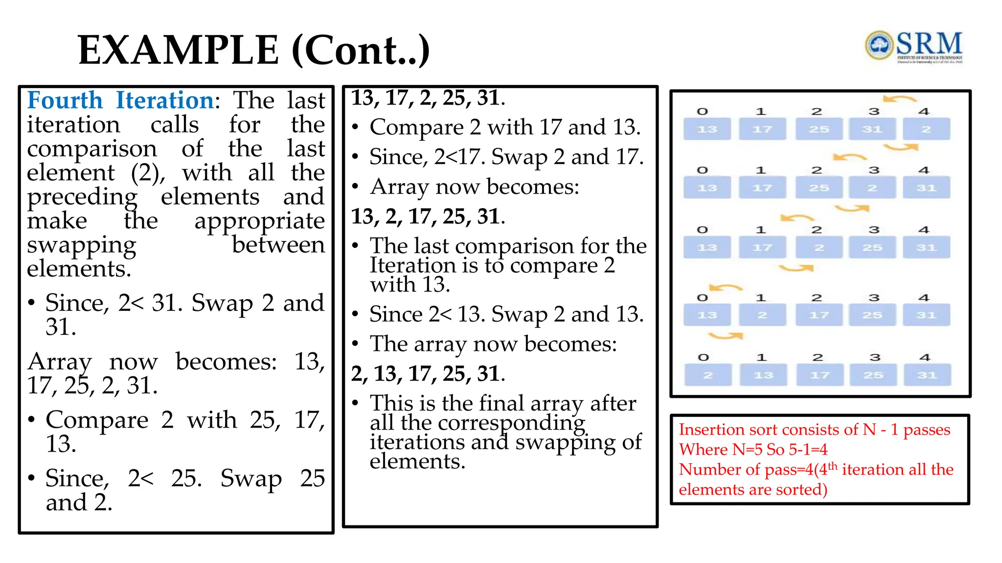
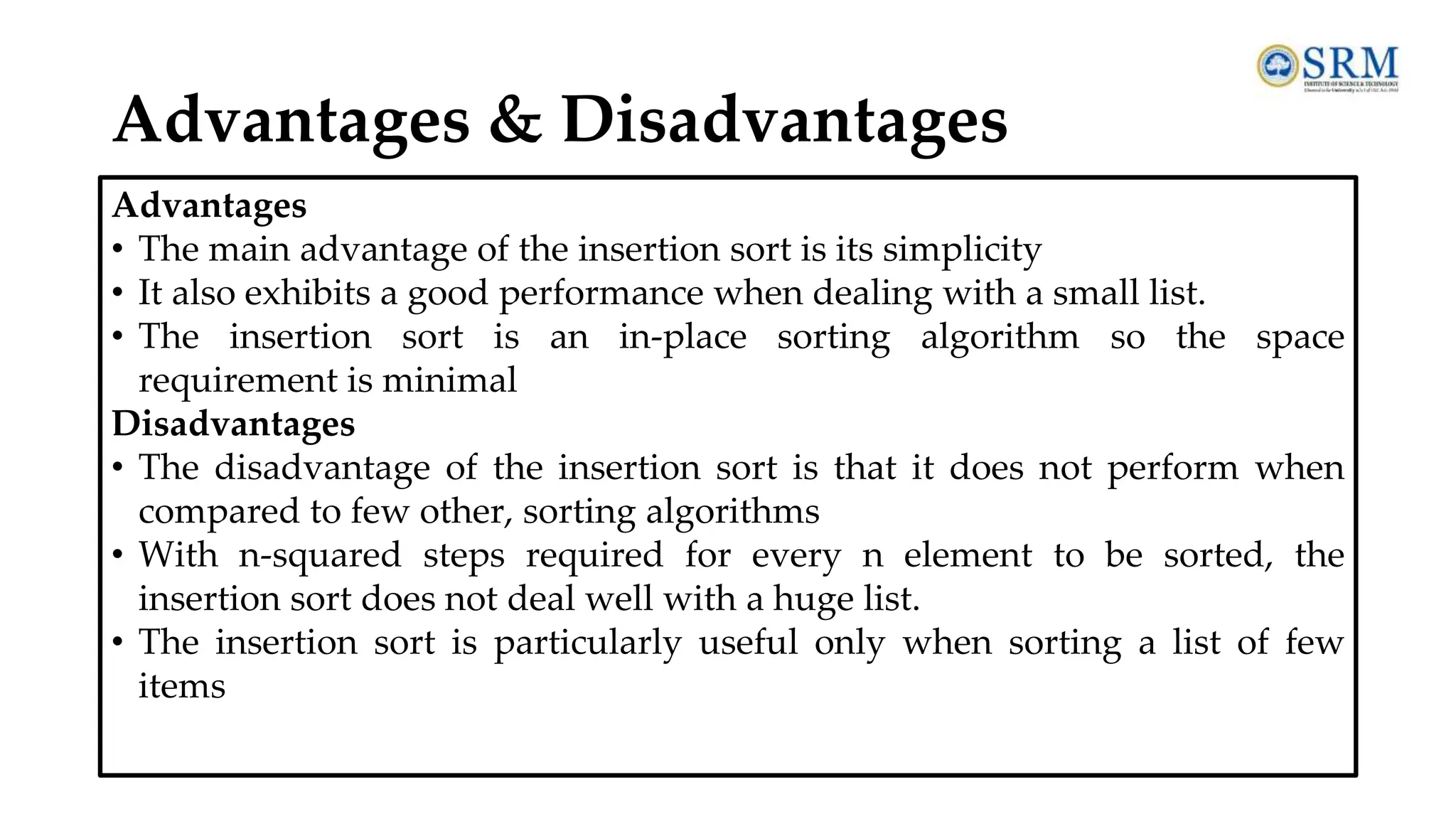
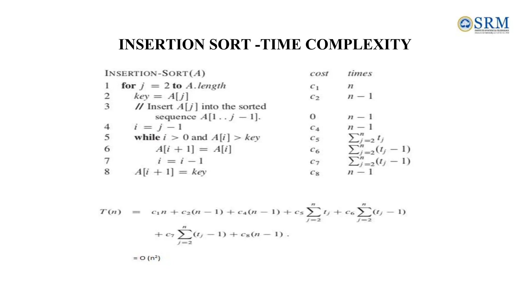
INSERTION SORT • Insertion sorts works by taking elements from the list one by one and inserting them in their current position into a new sorted list. • Insertion sort consists of N - 1 passes, where N is the number of elements to be sorted. • The ith pass of insertion sort will insert the ith element A[i] into its rightful place among A[1], A[2] to A[i - 1]. After doing this insertion the records occupying A[1]....A[i] are in sorted order. Pseudo code INSERTION-SORT(A) for i = 1 to n key ← A [i] j ← i – 1 while j > = 0 and A[j] > key A[j+1] ← A[j] j ← j – 1 End while A[j+1] ← key End for

Working of insertion sort – Ascending order • We start by considering the second element of the given array, i.e. element at index 1, as the key. • We compare the key element with the element(s) before it, i.e., element at index 0: – If the key element i.e index 1 is less than the first element, we insert the key element before the first element.(swap) – If the key element is greater than the first element, then we insert it remains at its position – Then, we make the third element of the array as key and will compare it with elements to it's left and insert it at the right position. • And we go on repeating this, until the array is sorted .

Example Let us now understand working with the following example: Consider the following array: 25, 17, 31, 13, 2 where N=5 First Iteration: Compare 17 with 25. The comparison shows 17< 25. Hence swap 17 and 25. The array now looks like: 17, 25, 31, 13, 2

EXAMPLE (Cont..) Second Iteration:. • Now hold on to the third element (31) and compare with the ones preceding it. • Since 31> 25, no swapping takes place. • Also, 31> 17, no swapping takes place and 31 remains at its position. • The array after the Second iteration looks like: 17, 25, 31, 13, 2

EXAMPLE (Cont..) Third Iteration: Start the following Iteration with the fourth element (13), and compare it with its preceding elements. • Since 13< 31, we swap the two. • Array now becomes: 17, 25, 13, 31, 2. • But there still exist elements that we haven’t yet compared with 13. Now the comparison takes place between 25 and 13. Since, 13 < 25, we swap the two. • The array becomes 17, 13, 25, 31, 2. • The last comparison for the iteration is now between 17 and 13. Since 13 < 17, we swap the two. • The array now becomes 13, 17, 25, 31, 2.

EXAMPLE (Cont..) Fourth Iteration: The last iteration calls for the comparison of the last element (2), with all the preceding elements and make the appropriate swapping between elements. • Since, 2< 31. Swap 2 and 31. Array now becomes: 13, 17, 25, 2, 31. • Compare 2 with 25, 17, 13. • Since, 2< 25. Swap 25 and 2. Insertion sort consists of N - 1 passes Where N=5 So 5-1=4 Number of pass=4(4th iteration all the elements are sorted) 13, 17, 2, 25, 31. • Compare 2 with 17 and 13. • Since, 2<17. Swap 2 and 17. • Array now becomes: 13, 2, 17, 25, 31. • The last comparison for the Iteration is to compare 2 with 13. • Since 2< 13. Swap 2 and 13. • The array now becomes: 2, 13, 17, 25, 31. • This is the final array after all the corresponding iterations and swapping of elements.

Advantages & Disadvantages Advantages • The main advantage of the insertion sort is its simplicity • It also exhibits a good performance when dealing with a small list. • The insertion sort is an in-place sorting algorithm so the space requirement is minimal Disadvantages • The disadvantage of the insertion sort is that it does not perform when compared to few other, sorting algorithms • With n-squared steps required for every n element to be sorted, the insertion sort does not deal well with a huge list. • The insertion sort is particularly useful only when sorting a list of few items

• The movement of air bubbles in the water that rise up to the surface, each element of the array move to the end in each iteration. Therefore, it is called a bubble sort. • Bubble sort is a simple sorting algorithm. This sorting algorithm is comparison-based algorithm in which each pair of adjacent elements is compared and the elements are swapped if they are not in order Steps to implement bubble sort: Assume that there are n elements in the list 1. In first cycle, 1. Start by comparing 1st and 2nd element and swap if they are not in order. 2. After that do the same for 2nd and 3rd element. Repeat till n-1th and nth elements are compared. 3. At the end of cycle one element (max/min) will be placed as the last element in of list. 2. The process specified in step 1 is repeated for another n-2 times, where in each time the number of comparisons reduce by 1 as the list of sorted elements grow. BUBBLE SORT

Working of Bubble Sort – Ascending order Suppose we are trying to sort the elements in ascending order. Let us now understand working with the following example: Consider the following array: -2,45,0,11,-9 where N=5 First Iteration (Compare and Swap) • Starting from the first index, compare the first and the second elements. • If the first element is greater than the second element, they are swapped. • Now, compare the second and the third elements. Swap them if they are not in order. • The above process goes on until the last element

Second Iteration • The same process goes on for the remaining iterations. • After each iteration, the largest element among the unsorted elements is placed at the end. Put the largest element at the end Working of Bubble Sort (Cont..)

Third Iteration In each iteration, the comparison takes place up to the last unsorted element. Compare the adjacent elements Fourth Iteration The array is sorted when all the unsorted elements are placed at their correct positions. The array is sorted if all elements are kept in the right order. Now all the elements are sorted Working of Bubble Sort (Cont..)

ADVANTAGES AND DISADVANTAGES Advantage: • It is the simplest sorting approach. • The primary advantage of the bubble sort is that it is popular and easy to implement. • In the bubble sort, elements are swapped in place without using additional temporary storage. Stable sort: does not change the relative order of elements with equal keys. • The space requirement is at a minimum Disadvantage: • Bubble sort is comparatively slower algorithm. • The main disadvantage of the bubble sort is the fact that it does not deal well with a list containing a huge number of items. • The bubble sort requires n-squared processing steps for every n number of elements to be sorted.

COMPLEXITY – TIME , SPACE TRADE OFF

SPACE COMPLEXITY • Space complexity is the total amount of memory space used by an algorithm/program including the space of input values for execution. So to find space-complexity, it is enough to calculate the space occupied by the variables used in an algorithm/program. • Space complexity S(P) of any algorithm P is, • S(P) = C + SP(I) • Where C is the fixed part and S(I) is the variable part of the algorithm which depends on instance characteristic I. Example: Algorithm: SUM(A, B) Step 1 - START Step 2 - C ← A + B + 10 Step 3 – Stop Here we have three variables A, B & C and one constant. Hence S(P) = 1+3. Space requirement depends on data types of given variables & constants. The number will be multiplied accordingly.

How to calculate Space Complexity of an Algorithm? • In the Example program, 3 integer variables are used. • The size of the integer data type is 2 or 4 bytes which depends on the architecture of the system (compiler). Let us assume the size as 4 bytes. • The total space required to store the data used in the example program is 4 * 3 = 12, Since no additional variables are used, no extra space is required. Hence, space complexity for the example program is O(1), or constant.

EXAMPLE 2 • In the code given above, the array stores a maximum of n integer elements. Hence, the space occupied by the array is 4 * n. Also we have integer variables such as n, i and sum. • Assuming 4 bytes for each variable, the total space occupied by the program is 4n + 12 bytes. • Since the highest order of n in the equation 4n + 12 is n, so the space complexity is O(n) or linear.

EXAMPLE 3 #include<stdio.h> int main() { int a = 5, b = 5, c; c = a + b; printf("%d", c); } Space Complexity: size(a)+size(b)+size(c) =>let sizeof(int)=2 bytes=>2+2+2=6 bytes =>O(1) or constant

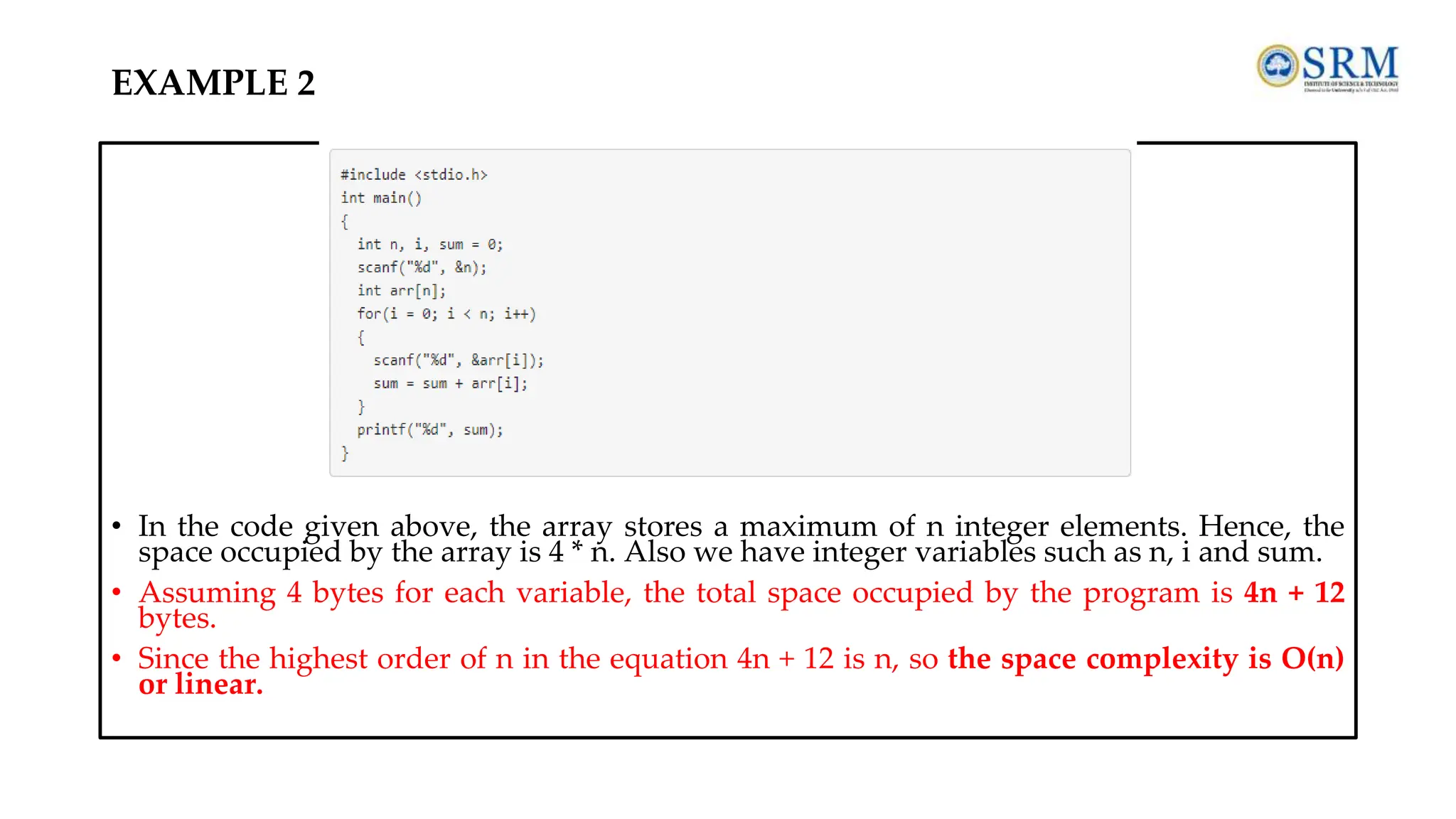
Example 4 #include <stdio.h> int main() { int n, i, sum = 0; scanf("%d", &n); int arr[n]; for(i = 0; i < n; i++) { scanf("%d", &arr[i]); sum = sum + arr[i]; } printf("%d", sum); } Space Complexity: • The array consists of n integer elements. • So, the space occupied by the array is 4 * n. Also we have integer variables such as n, i and sum. Assuming 4 bytes for each variable, the total space occupied by the program is 4n + 12 bytes. • Since the highest order of n in the equation 4n + 12 is n, so the space complexity is O(n) or linear.

• Time Complexity of an algorithm represents the amount of time required by the algorithm to run to completion. • Time requirements can be defined as a numerical function T(n), where T(n) can be measured as the number of steps, provided each step consumes constant time. • Eg. Addition of two n-bit integers takes n steps. • Total computational time is T(n) = c*n, • where c is the time taken for addition of two bits. • Here, we observe that T(n) grows linearly as input size increases. Time Complexity

Time Complexity (Cont..) Two methods to find the time complexity for an algorithm 1. Count variable method 2. Table method 9/11/21 71

Table Method • The table contains s/e and frequency. • The s/e of a statement is the amount by which the count changes as a result of the execution of that statement. • Frequency is defined as the total number of times each statement is executed. • Combining these two, the step count for the entire algorithm is obtained. 73 9/11/21

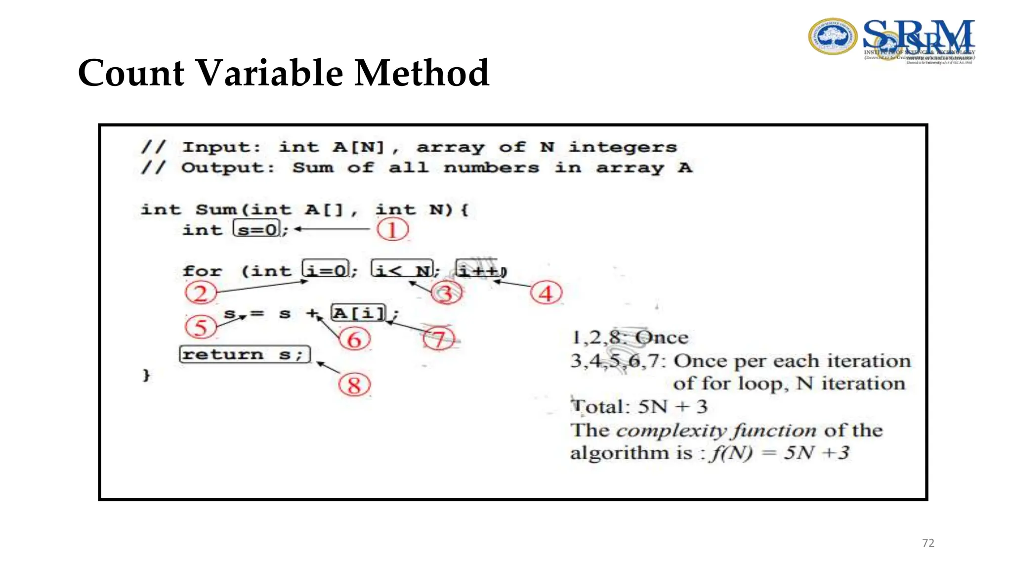
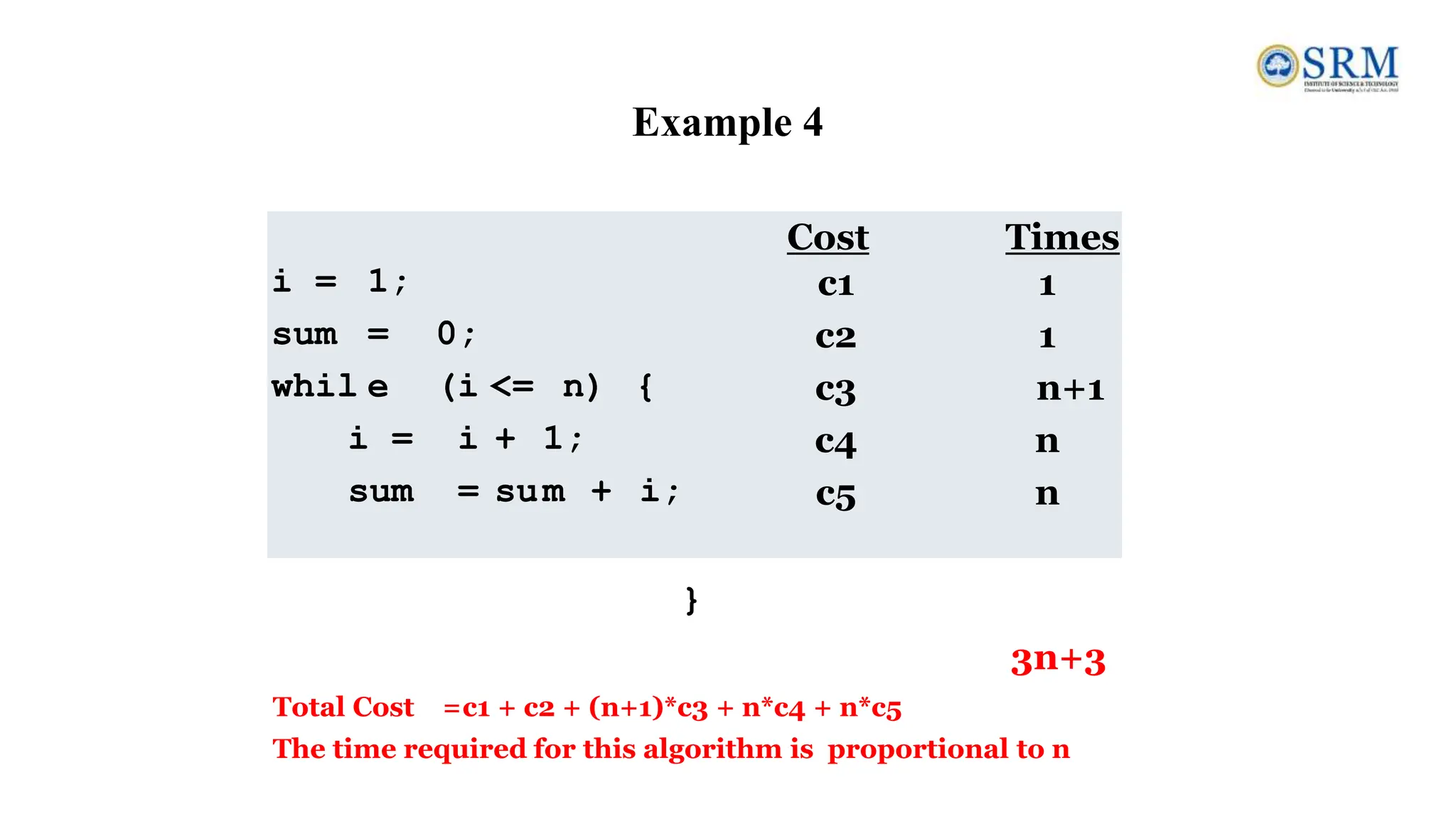
int sum(int A[], int n) { int sum = 0, i; for(i = 0; i < n; i++) sum = sum + A[i]; return sum; } • In above calculation Cost is the amount of computer time required for a single operation in each line. • Repetition is the amount of computer time required by each operation for all its repetitions. • Total is the amount of computer time required by each operation to execute. So above code requires '4n+4' Units of computer time to complete the task. Here the exact time is not fixed. And it changes based on the n value. If we increase the n value then the time required also increases linearly. Totally it takes '4n+4' units of time to complete its execution Example 2

Example 3 Consider the following piece of code... int sum(int a, int b) { return a+b; } In the above sample code, it requires 1 unit of time to calculate a+b and 1 unit of time to return the value. That means, totally it takes 2 units of time to complete its execution. And it does not change based on the input values of a and b. That means for all input values, it requires the same amount of time i.e. 2 units. If any program requires a fixed amount of time for all input values then its time complexity is said to be Constant Time Complexity

Cost Times i = 1; c1 1 sum = 0; c2 1 whil e (i <= n) { c3 n+1 i = i + 1; c4 n sum = sum + i; c5 n } 3n+3 Total Cost =c1 + c2 + (n+1)*c3 + n*c4 + n*c5 The time required for this algorithm is proportional to n Example 4

Total Cost = c1 + c2 + (n+1)*c3 + n*c4 + n*(n+1)*c5+n*n*c6+n*n*c7+n*c8 The time required for this algorithm is proportional to n2 Example 5

INSERTION SORT -TIME COMPLEXITY

Time Complexity of Bubble Sort

Review Questions Sort the following numbers using bubble sort and Insertion sort • 35,12,14,9,15,45,32,95,40,5 • 3, 1, 4, 1, 5, 9, 2, 6, 5 • 17 14 34 26 38 7 28 32 • 35,12,14,9,15,45,32,95,40,5

Review questions 83 1. Calculate the time complexity for the below algorithms using table method

1. Floor and Ceiling Functions

2. Remainder Function (Modular Arithmetic)

3. Integer and Absolute Value Functions

ASYMPTOTIC NOTATIONS BIG O, OMEGA

Asymptotic Analysis • The time required by an algorithm falls under three types − • Best Case − Minimum time required for program execution. • Average Case − Average time required for program execution. • Worst Case − Maximum time required for program execution. 94

Asymptotic Analysis (Cont..) • Asymptotic analysis of an algorithm refers to defining the mathematical boundation/framing of its run-time performance. • Derive the best case, average case, and worst case scenario of an algorithm. • Asymptotic analysis is input bound. • Specify the behaviour of the algorithm when the input size increases • Theory of approximation. • Asymptote of a curve is a line that closely approximates a curve but does not touch the curve at any point of time. 95

Asymptotic notations • Asymptotic notations are mathematical tools to represent the time complexity of algorithms for asymptotic analysis. • Asymptotic order is concerned with how the running time of an algorithm increases with the size of the input, if input increases from small value to large values 1. Big-Oh notation (O) 2. Big-Omega notation (Ω) 3. Theta notation (θ) 4. Little-oh notation (o) 5. Little-omega notation (ω) 96 9/11/21

Big-Oh Notation (O) • Big-oh notation is used to define the worst-case running time of an algorithm and concerned with large values of n. • Definition: A function t(n) is said to be in O(g(n)), denoted as t(n) ϵ O(g(n)), if t(n) is bounded above by some constant multiple of g(n) for all large n. i.e., if there exist some positive constant c and some non-negative integer n0 such that t(n) ≤ cg(n) for all n ≥ n0 • O(g(n)): Class of functions t(n) that grow no faster than g(n). • Big-oh puts asymptotic upper bound on a function. 9/11/21 97

Big-Oh Notation (O) 9/11/21 98

Big-Oh Notation (O) 1 < log n < √n < n < n logn < n2 < n3 < ……………< 2n < 3n < …. <nn • Let t(n) = 2n + 3 upper bound 2n + 3 ≤ _____?? 2n + 3 ≤ 5n n ≥ 1 here c = 5 and g(n) = n t(n) = O(n) 2n + 3 ≤ 5n2 n ≥ 1 here c = 5 and g(n) = n2 t(n) = O(n2 ) 99

Big-Omega notation (Ω) • This notation is used to describe the best case running time of algorithms and concerned with large values of n. • Definition: A function t(n) is said to be in Ω(g(n)), denoted as t(n) ϵ Ω(g(n)), if t(n) is bounded below by some positive constant multiple of g(n) for all large n. i.e., there exist some positive constant c and some non-negative integer n0. Such that t(n) ≥cg(n) for all n ≥ n0 • It represents the lower bound of the resources required to solve a problem. 9/11/21 100

Big-Omega notation (Ω) 9/11/21 101

Big-Omega notation (Ω) 1 < log n < √n < n < n logn < n2 < n3 < ……………< 2n < 3n < …. <nn • Let t(n) = 2n + 3 lower bound 2n + 3 ≥ _____?? 2n + 3 ≥ 1n n ≥ 1 here c = 1 and g(n) = n t(n) = Ω(n) 2n + 3 ≥ 1log n n ≥ 1 here c = 1 and g(n) = log n t(n) = Ω(log n) 9/11/21 102

Asymptotic Analysis of Insertion sort • Time Complexity: • Best Case: the best case occurs if the array is already sorted, tj=1 for j=2,3…n. • Linear running time: O(n) 9/11/21 103

Asymptotic Analysis of Insertion sort • Worst case : If the array is in reverse sorted order • Quadratic Running time. O(n2) 9/11/21 104

Properties of O, Ω and θ General property: If t(n) is O(g(n)) then a * t(n) is O(g(n)). Similar for Ω and θ Transitive Property : If f (n) ϵ O(g(n)) and g(n) ϵ O(h(n)), then f (n) ϵ O(h(n)); that is O is transitive. Also Ω, θ, o and ω are transitive. Reflexive Property If f(n) is given then f(n) is O(f(n)) Symmetric Property If f(n) is θ(g(n)) then g(n) is θ(f(n)) Transpose Property If f(n) = O(g(n)) then g(n) is Ω(f(n)) 9/11/21 105

Review Questions • Indicate constant time complexity in terms of Big-O notation. A. O(n) B. O(1) C. O(logn) D. O(n^2) • Big oh notation is used to describe __________ • Big O Notation is a _________function used in computer science to describe an ____________ • Big Omega notation (Ω) provides _________bound. • Given T1(n) =O(f(n)) and T2(n)=O(g(n).Find T1(n).T2(n) 106

ASYMPTOTIC NOTATION-THETA MATHEMATICAL FUNCTIONS

Asymptotic Notation – THETA Θ

Example - THETA • Show that n2 /2 – 2n = Θ(n2 ).

Mathematical Functions (Cont..)

Review Questions 1. Give examples of functions that are in Θ notation as well as functions that are not in Θ notation. 2. Which function gives the positive value of the given input? 3. K (mod) M gives the reminder of ____ divided by ____ 4. For a given set of number n, the number of possible permutation will be equal to the ____________ value of n. 5. ________Notation is used to specify both the lower bound and upper bound of the function.

Data Structure • A data structure is basically a group of data elements that are put together under one name • Defines a particular way of storing and organizing data in a computer so that it can be used efficiently • Data Structures are used in ∙ Compiler design ∙ Operating system ∙ Statistical analysis package ∙ DBMS • The selection of an appropriate data structure provides the most efficient solution

Terms in Data Structure • Data: Data can be defined as an elementary value or the collection of values, for example, student's name and its id are the data about the student. • Group Items: Data items which have subordinate data items are called Group item, for example, name of a student can have first name and the last name. • Record: Record can be defined as the collection of various data items, for example, if we talk about the student entity, then its name, address, course and marks can be grouped together to form the record for the student. • File: A File is a collection of various records of one type of entity, for example, if there are 60 employees in the class, then there will be 20 records in the related file where each record contains the data about each employee. • Attribute and Entity: An entity represents the class of certain objects. it contains various attributes. Each attribute represents the particular property of that entity. • Field: Field is a single elementary unit of information representing the attribute of an entity.

Types of Data Structure Primitive Data Structures: Primitive data structures are the fundamental data types which are supported by a programming language. Some basic data types are ∙ Integer ∙ Real ∙ Character ∙ Boolean Non-Primitive Data Structures: Non-primitive data structures are those data structures which are created using primitive data structures. Examples of such data structures include ∙ linked lists ∙ stacks ∙ trees ∙ graphs

LINEAR AND NON- LINEAR DATA STRUCTURES

Types of Data Structure – Non Primitive Linear Arrays • An array is a collection of similar type of data items and each data item is called an element of the array. Linked List • Dynamic data structure in which elements (called nodes) form a sequential list

Types of Data Structure – Non Primitive Linear Stack • Linear data structure in which insertion and deletion of elements are done at only one end, which is known as the top of the stack Queue • Linear data structure in which the element that is inserted first is the first one to be taken out

Types of Data Structure – Non Primitive - Non Linear • The data structure where data items are not organized sequentially is called non linear data structure • Types • Trees • Graphs

Types of Data Structure – Non Primitive - Non Linear TREES • A tree is a non-linear data structure which consists of a collection of nodes arranged in a hierarchical order. • One of the nodes is designated as the root node, and the remaining nodes can be partitioned into disjoint sets such that each set is a sub-tree of the root.

Types of Data Structure – Non Primitive - Non Linear GRAPHS • A graph is a non-linear data structure which is a collection of vertices (also called nodes) and edges that connect these vertices. • A graph is often viewed as a generalization of the tree structure. • every node in the graph can be connected with another node in the graph. • When two nodes are connected via an edge, the two nodes are known as neighbours.

Review Questions 1. Compare a linked list with an array. 2. Is Array static structure or dynamic structure (TRUE / FALSE) 3. The data structure used in hierarchical data model is _________ 4. In a stack, insertion is done at __________ 5. Which Data Structure follows the LIFO fashion of working? 6. The position in a queue from which an element is deleted is called as __________

Definition and Features of Pointer ⮚Definition: • Pointer is a variable that stores the address of another variable. ⮚Features • Pointer saves the memory space. • Execution time of pointer is faster because of direct access to the memory location. • With the help of pointers, the memory is accessed efficiently, i.e., memory is allocated and deallocated dynamically. • Pointers are used with data structures.

Pointer declaration, initialization and accessing • Consider the following statement int q = 159; In memory, the variable can be represented as follows − 159 q 1000 Variable Value Address

Pointer declaration, initialization and accessing(Cont..) • Declaring a pointer It means ‘p’ is a pointer variable which holds the address of another integer variable, as mentioned in the statement below − int *p; • Initialization of a pointer Address operator (&) is used to initialise a pointer variable. For example − int q = 159; int *p; p= &q; Variable Value Address q p 159 1000 1000 2000

• Accessing a variable through its pointer To access the value of a variable, indirection operator (*) is used. For example − int q=159, *p,n; p=&q; n=*p Here, ‘*’ can be treated as value at address. p = &q; n = *p; n =q Pointer declaration, initialization and accessing(Cont..)

1D INITIALIZATION & ACCESSING USING POINTERS

⮚The compiler allocates Continuous memory locations for all the elements of the array. ⮚The base address = first element address (index 0) of the array. ⮚Syntax: data_type (var_name)[size_of_array] • For Example − int a [5] = {10, 20,30,40,50}; ⮚Elements • The five elements are stored as follows − Pointers and one-dimensional arrays Elements a[0] a[1] a[2] a[3] a[4] Values 10 20 30 40 50 Address 1000 1004 1008 1012 1016 Base Address a=&a[0]=1000 //Declaration int *p; int my_arr[] = {11, 22, 33, 44, 55}; p = my_arr;

• If ‘p’ is declared as integer pointer, then, an array ‘a’ can be pointed by the following assignment − p = a; (or) p = &a[0]; • Every value of 'a' is accessed by using p++ to move from one element to another element. When a pointer is incremented, its value is increased by the size of the data type that it points to. This length is called the "scale factor". • The relationship between ‘p’ and 'a' is explained below P = &a[0] = 1000 P+1 = &a[1] = 1004 P+2 = &a[2] = 1008 P+3 = &a[3] = 1012 P+4 = &a[4] = 1016 Pointers and one-dimensional arrays (Cont)

• Address of an element is calculated using its index and the scale factor of the data type. An example to explain this is given herewith. • Address of a[3] = base address + (3* scale factor of int) = 1000 + (3*4) = 1000 +12 = 1012 • Pointers can be used to access array elements instead of using array indexing. • *(p+3) gives the value of a[3]. • a[i] = *(p+i) Pointers and one-dimensional arrays (Cont..)

•Following is the C program for pointers and one-dimensional arrays − #include<stdio.h> main ( ) { int a[5]; int *p,i; printf ("Enter 5 lements"); for (i=0; i<5; i++) scanf ("%d", &a[i]); p = &a[0]; printf ("Elements of the array are"); for (i=0; i<5; i++) printf("%d", *(p+i)); } Output When the above program is executed, it produces the following result − Enter 5 elements : 10 20 30 40 50 Elements of the array are : 10 20 30 40 50 Example Program

POINTER ARRAYS Syntax: data_type (*var_name)[size_of_array] •Example: int (*arr_ptr)[5], *a_ptr, arr[5][5] ={{10,20,30,23,12}, {15,25,35,33,88}, {45,25,77,57,54}, {65,34,67,33,99}, {44,45,55,44,65}}; arr_ptr= & arr; a_ptr= & arr; arr_ptr++; a_ptr++; Example Program 1020 10 1024 20 1028 30 1032 23 1036 12 1040 15 1044 25 1048 35 1052 33 1056 88 1060 45 1064 25 1068 77 1072 57 1076 54 1080 65 1084 34 1088 67 1092 33 1096 99 1100 44 1104 45 1108 55 1112 44 1116 65 arr_ptr a_ptr

Example Program : 1D array using Pointer #include<stdio.h> int main() { int array[5]; int i,sum=0; int *ptr; printf("nEnter array elements (5 integer values):"); for(i=0;i<5;i++) scanf("%d",&array[i]); /* array is equal to base address * array = &array[0] */ ptr = array; for(i=0;i<5;i++) { //*ptr refers to the value at addresssum = sum + *ptr; ptr++; } printf("nThe sum is: %d",sum); } Output Enter array elements (5 integer values): 1 2 3 4 5 The sum is: 15

2D INITIALIZATION & ACCESSING USING POINTERS

Pointers and two-dimensional arrays • Memory allocation for a two-dimensional array is as follows − int a[3] [3] = {1,2,3,4,5,6,7,8,9}; 1 2 3 4 5 6 7 8 9 0 1 2 0 1 2 Row 1-> 1 2 3 a[0][0] a[0][1] a[0][2] 1000 1004 1008 Row 2-> 4 5 6 a[1][0] a[1][1] a[1][2] 1012 1016 1020 Row 1-> 7 8 9 a[2][0] a[2][1] a[2][2] 1024 1028 1032 Base Address=1000=&a[0][0]

Pointers and two-dimensional arrays • Assigning Base Address to pointer int *p p=&a[0][0] (or) p=a Pointer is used to access the elements of 2-dimensional array as follows a[i][j]=*(p+j *columnsize+j) a[1] [2] = *(1000 + 1*3+2) = *(1000 + 3+2) = *(1000 + 5*4) // 4 is Scale factor = * (1000+20) = *(1020) a[1] [2] = 6

Example Program #include<stdio.h> main ( ) { int a[3] [3], i,j; int *p; clrscr ( ); printf ("Enter elements of 2D array"); for (i=0; i<3; i++) { for (j=0; j<3; j++) { scanf ("%d", &a[i] [j]); } } p = &a[0] [0]; printf ("elements of 2d array are"); for (i=0; i<3; i++) { for (j=0; j<3; j++) { printf ("%d t", *(p+i*3+j)); } printf ("n"); } getch ( ); } Output When the above program is executed, it produces the following result − enter elements of 2D array 1 2 3 4 5 6 7 8 9 Elements of 2D array are 1 2 3 4 5 6 7 8 9

Review Questions 1. Let’s consider 60 students took this course. Each student is supposed to give a rating 1, 2, 3 4 or 5; one being bad and 5 being good. Find the ratings are spread count the number of times each rating was given. 2. Write a Program in C for the following Array operations a. Creating an Array of N Integer Elements b. Display of Array Elements with Suitable Headings c. Inserting an Element (ELEM) at a given valid Position (POS) d. Deleting an Element at a given valid Position(POS) e. Exit. Support the program with functions for each of the above operations.

DECLARING STRUCTURE AND ACCESSING

Definition of Structures • Structures are user defined data types • It is a collection of heterogeneous data • It can have integer, float, double or character data in it • We can also have array of structures struct<<structname>> { members; }element; We can access element.members;

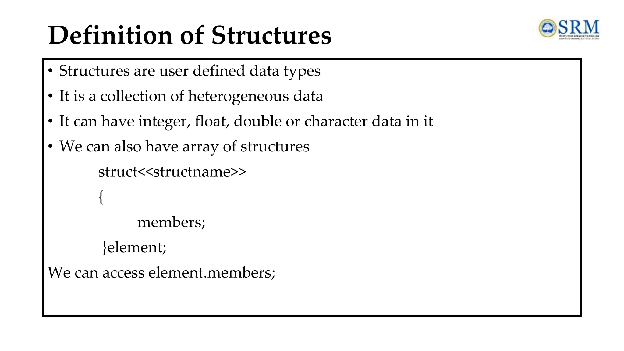
Declaration of Structures Syntax: struct struct_Name • { • <data-type> member_name; • <data-type> member_name; • … • } list of variables; Example: Structure to hold student details struct Student { int regNo; char name[25]; int english, science, maths; } stud;

Declaration of Structures Syntax: struct struct_Name { <data-type> member_name; <data-type> member_name; … }; struct struct_Name struct_var; struct Student { int regNo; char name[25]; int english, science, maths; }; struct Student stud;

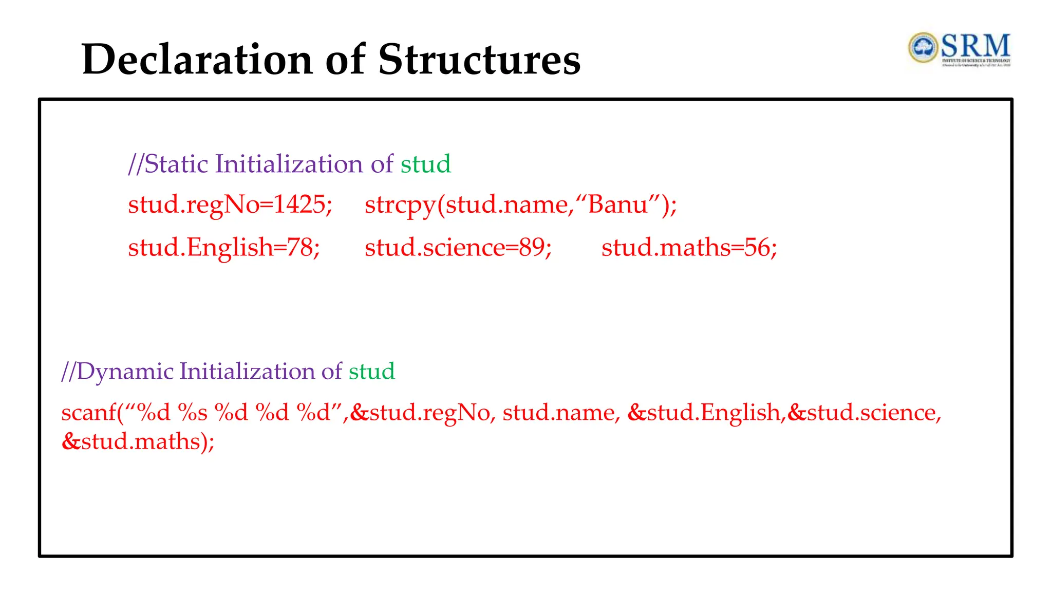
Declaration of Structures //Static Initialization of stud stud.regNo=1425; strcpy(stud.name,“Banu”); stud.English=78; stud.science=89; stud.maths=56; //Dynamic Initialization of stud scanf(“%d %s %d %d %d”,&stud.regNo, stud.name, &stud.English,&stud.science, &stud.maths);

Accessing and Updating Structures struct Student { int regNo; char name[25]; int english, science, maths; }; struct Student stud; scanf(“%d %s %d %d %d”,&stud.regNo, stud.name, &stud.english,&stud.science, &stud.maths); printf("Register number =% dn",stud.Regno); printf("Name %s",stud.name); stud.english= stud.english +10; stud.science++; //Accessing member Regno //Accessing member name //Updating member english

Nested Structures struct Student { int regNo; char name[25]; struct marks { int english, science, maths; } } Amar; Amar.regNo; Amar.marks.english ; Amar.marks.science ; Amar.marks.maths; struct Student { int regNo; char name[25]; struct m marks; } Amar; struct m { int english; int science; int maths; }; struct Student { int regNo; char name[25]; struct {int english, science, maths } marks; } Amar;

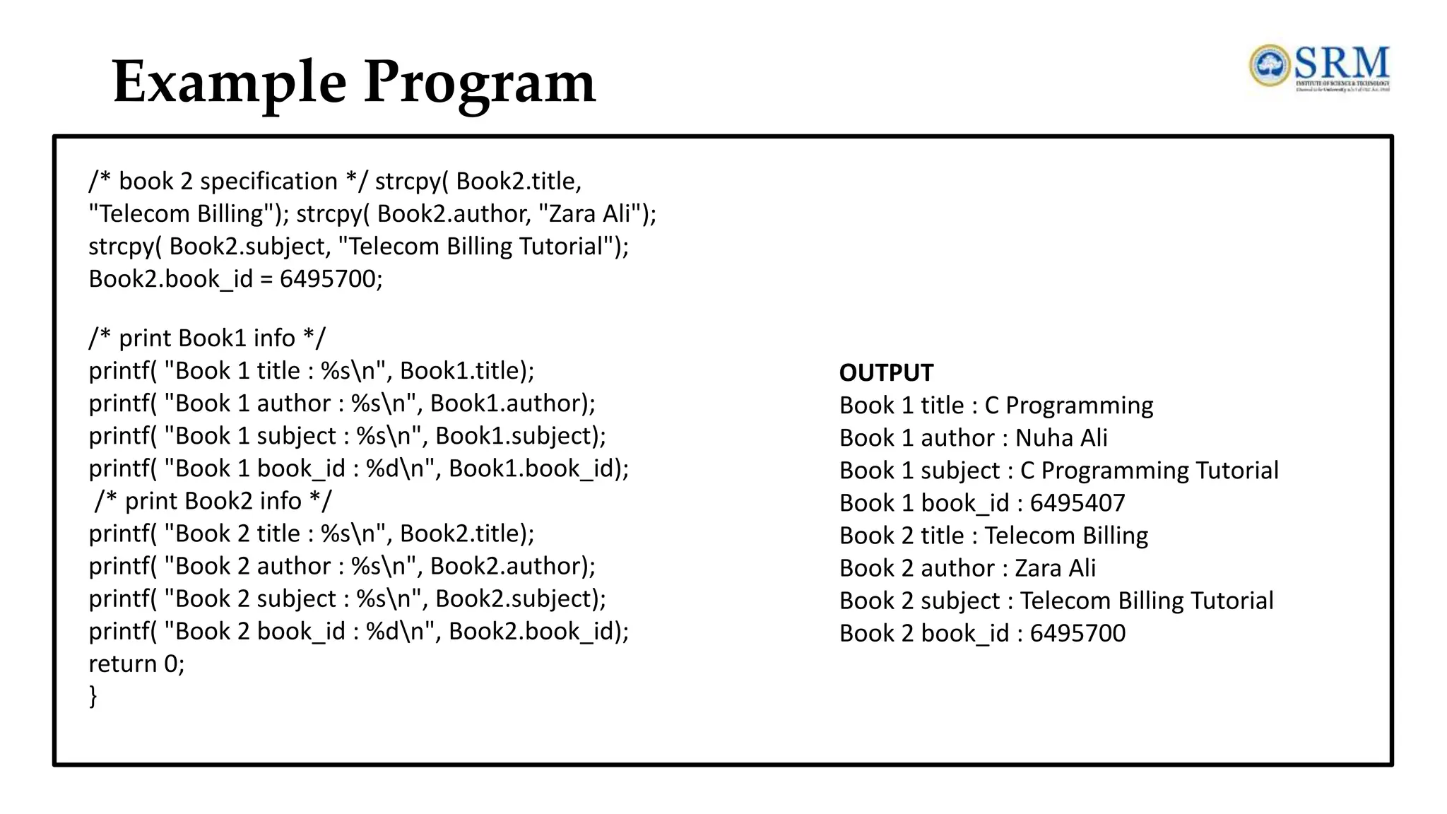
Example Program #include <stdio.h> #include <string.h> struct Books { char title[50]; char author[50]; char subject[100]; int book_id; }; /* book 1 specification */ strcpy( Book1.title, "C Programming"); strcpy( Book1.author, "Nuha Ali"); strcpy( Book1.subject, "C Programming Tutorial"); Book1.book_id = 6495407 int main( ) { struct Books Book1; /* Declare Book1 of type Book */ struct Books Book2; /* Declare Book2 of type Book */

Example Program /* book 2 specification */ strcpy( Book2.title, "Telecom Billing"); strcpy( Book2.author, "Zara Ali"); strcpy( Book2.subject, "Telecom Billing Tutorial"); Book2.book_id = 6495700; /* print Book1 info */ printf( "Book 1 title : %sn", Book1.title); printf( "Book 1 author : %sn", Book1.author); printf( "Book 1 subject : %sn", Book1.subject); printf( "Book 1 book_id : %dn", Book1.book_id); /* print Book2 info */ printf( "Book 2 title : %sn", Book2.title); printf( "Book 2 author : %sn", Book2.author); printf( "Book 2 subject : %sn", Book2.subject); printf( "Book 2 book_id : %dn", Book2.book_id); return 0; } OUTPUT Book 1 title : C Programming Book 1 author : Nuha Ali Book 1 subject : C Programming Tutorial Book 1 book_id : 6495407 Book 2 title : Telecom Billing Book 2 author : Zara Ali Book 2 subject : Telecom Billing Tutorial Book 2 book_id : 6495700

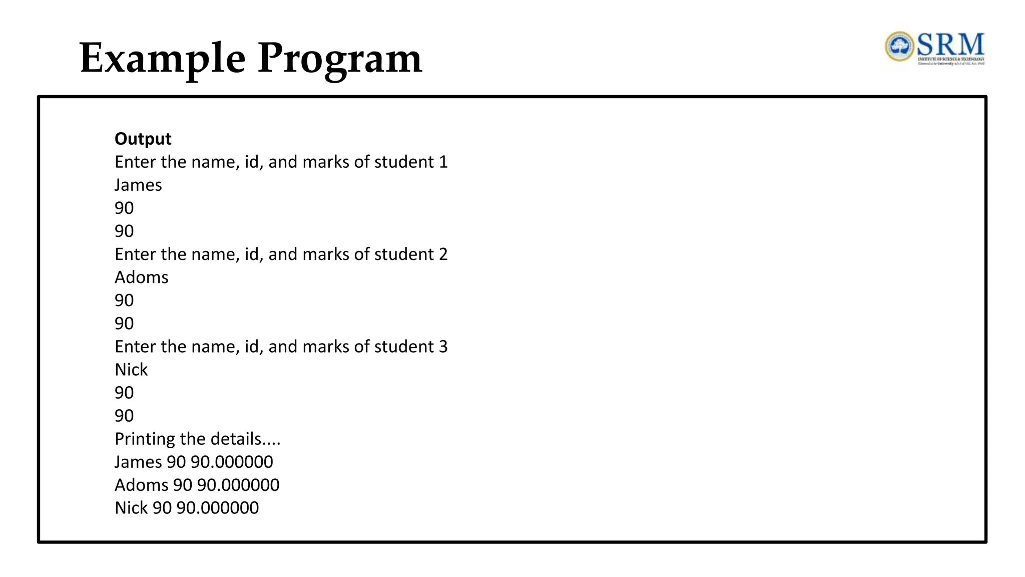
Example Program #include<stdio.h> struct student { char name[20]; int id; float marks; }; void main() { struct student s1,s2,s3; int dummy; printf("Enter the name, id, and marks of student 1 "); scanf("%s %d %f",s1.name,&s1.id,&s1.marks); scanf("%c",&dummy); printf("Enter the name, id, and marks of student 2 "); scanf("%s %d %f",s2.name,&s2.id,&s2.marks); scanf("%c",&dummy); printf("Enter the name, id, and marks of student 3 "); scanf("%s %d %f",s3.name,&s3.id,&s3.marks); scanf("%c",&dummy); printf("Printing the details....n"); printf("%s %d %fn",s1.name,s1.id,s1.marks); printf("%s %d %fn",s2.name,s2.id,s2.marks); printf("%s %d %fn",s3.name,s3.id,s3.marks); }

Example Program Output Enter the name, id, and marks of student 1 James 90 90 Enter the name, id, and marks of student 2 Adoms 90 90 Enter the name, id, and marks of student 3 Nick 90 90 Printing the details.... James 90 90.000000 Adoms 90 90.000000 Nick 90 90.000000

DECLARING ARRAY OF STRUCTURES AND ACCESSING

Array of Structures struct Student { int regNo; char name[25]; int english, science, maths; }; struct Student stud[10]; scanf(“%d%s%d%d%d”,&stud[1].regNo,stud[1].name,&stud[1].english,&stu d[1].science, &stud[1].maths); printf("Register number = %dn",stud[1].Regno); printf("Name %s",stud[1].name); stud.[1]english= stud[0].english +10; stud[1].science++; //Accessing member Regno //Accessing member name //Updating member english

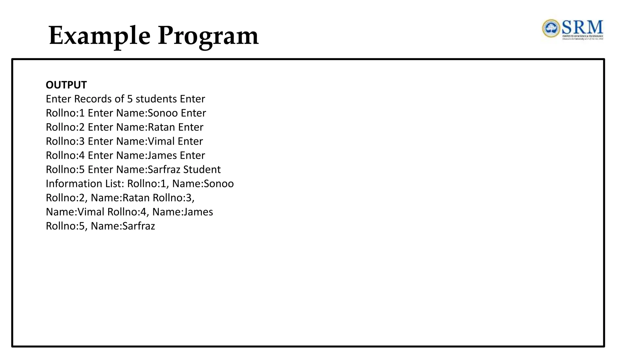
Example Program #include<stdio.h> #include <string.h> struct student{ int rollno; char name[10]; }; int main() { int i; struct student st[5]; printf("Enter Records of 5 students"); for(i=0;i<5;i++){ printf("nEnter Rollno:"); scanf("%d",&st[i].rollno); printf("nEnter Name:"); scanf("%s",&st[i].name); } printf("nStudent Information List:"); for(i=0;i<5;i++){ printf("nRollno:%d, Name:%s",st[i].rollno,st[i].name); } return 0; }

Example Program OUTPUT Enter Records of 5 students Enter Rollno:1 Enter Name:Sonoo Enter Rollno:2 Enter Name:Ratan Enter Rollno:3 Enter Name:Vimal Enter Rollno:4 Enter Name:James Enter Rollno:5 Enter Name:Sarfraz Student Information List: Rollno:1, Name:Sonoo Rollno:2, Name:Ratan Rollno:3, Name:Vimal Rollno:4, Name:James Rollno:5, Name:Sarfraz

Review Questions 1. Write a C program for student mark sheet using structure 2. Write a C program using structure to find students grades in a class 3. Write a C program for book details using structure 4. Calculating the area of a rectangle using structures in C language.

Data structure and algorithms unit 1 pdf SRM

More Related Content

What's hot

Similar to Data structure and algorithms unit 1 pdf SRM

Recently uploaded

Data structure and algorithms unit 1 pdf SRM