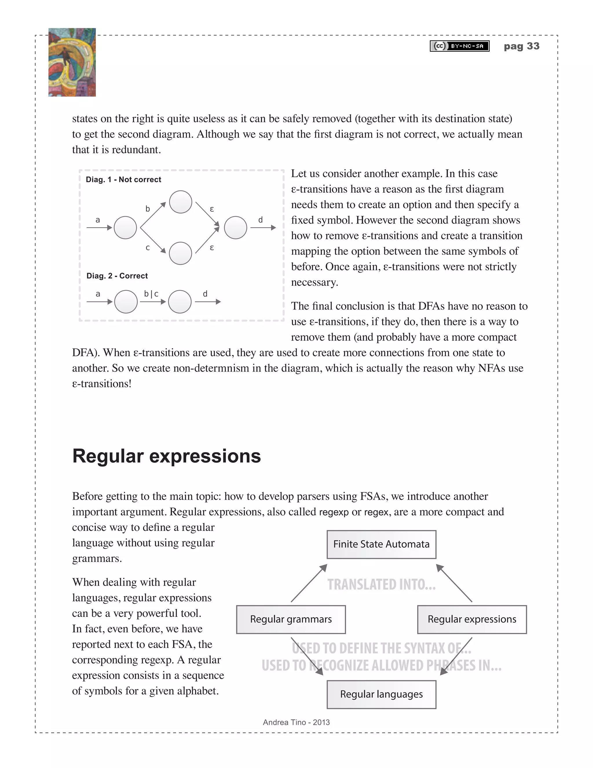
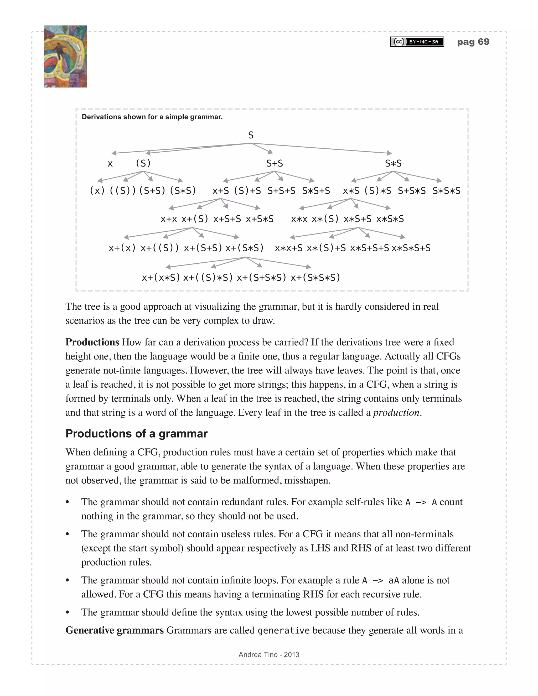
Downloaded 56 times
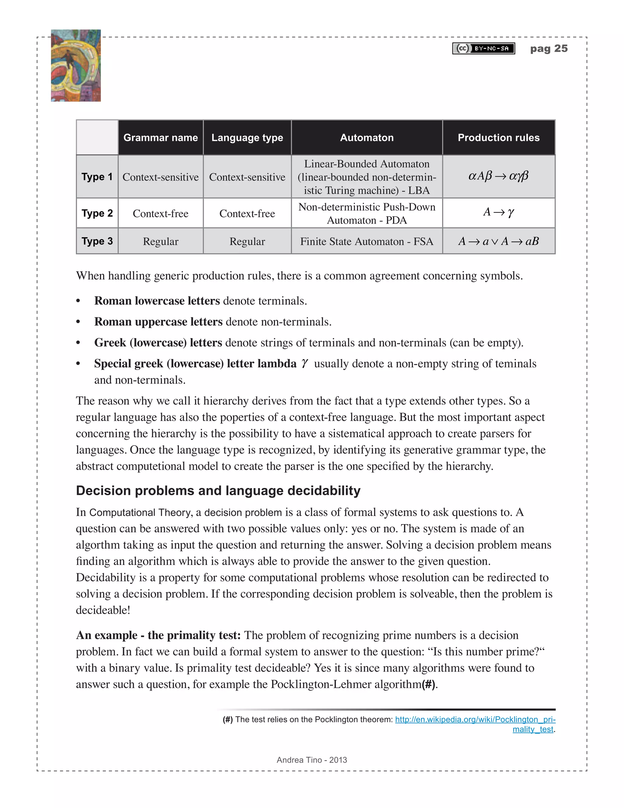
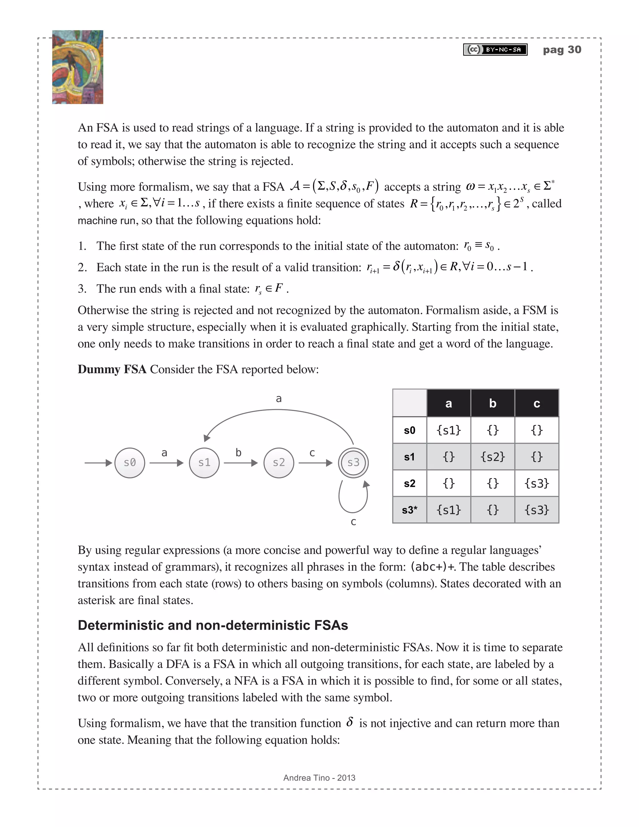
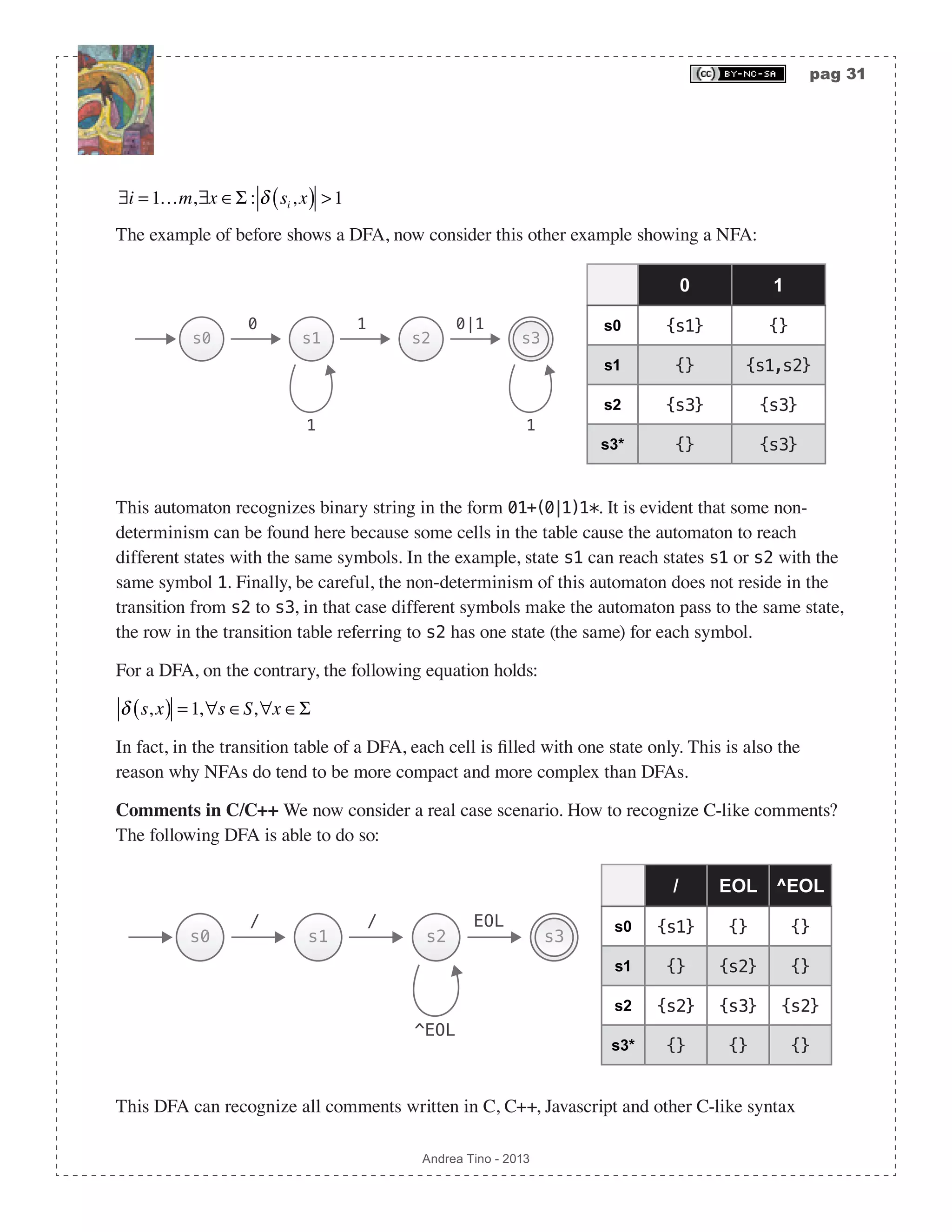
![pag 29 Andrea Tino - 2013 A very important theorem relates finite languages with regular languages. [Theo] Language finiteness theorem: A finite language is also a regular language. Please note that the inverse is not true, if a language is regular it is not said that it is finite. For this reason some algorithms are used to check whether a language is regular or not. Deciding whether a language is regular The problem of telling whether a language is regular or not is a decision problem. Such a problem is decidable and some approaches can be used to check whether or not a language is regular. One of the most common is the Myhill-Nerode theorem. A parser for regular languages Regular languages can be parsed, according to the Chomsky-Schützenberger hierarchy, by FSAs. In fact the decision problem for regular languages can be solved by FSAs. We can have two types of FSAs: • Deterministic: DFA or DFSA. They are fast but can be less compact. • Non-deterministic: NFA or NFSA. They are not as fast, but more compact in most cases. Both of them can be used to recognize phrases of a regular language. When developing lexers for a generic language, DFAs are used. Finite State Automata (FSA) They are also called Finite State Machines (FSM). Since a regular language can be parsed by an FSA, we need to study these abstract computational models. A generic FSA (deterministic or non- deterministic) can be defined as a 5-tuple A = Σ,S,δ,s0,F( ). • A finite set of symbols denoted by Σ = a1,a2,…,an{ } and called Alphabet. • A finite set of states denoted by S = s0,s1,s2,…,sm{ }. • A transition function denoted by δ :S × Σ 2S , responsible for selecting the next active state of the automaton. The function can be described as a table states/symbols whose entries are subsets of the symbols set. • A special state denoted by s0 ∈S and called initial state. • A subset of states denoted by F ⊆ S whose members are called final states.](https://image.slidesharecdn.com/creatingacompilerforyourownlanguage-150105162410-conversion-gate01/75/Creating-a-compiler-for-your-own-language-29-2048.jpg)
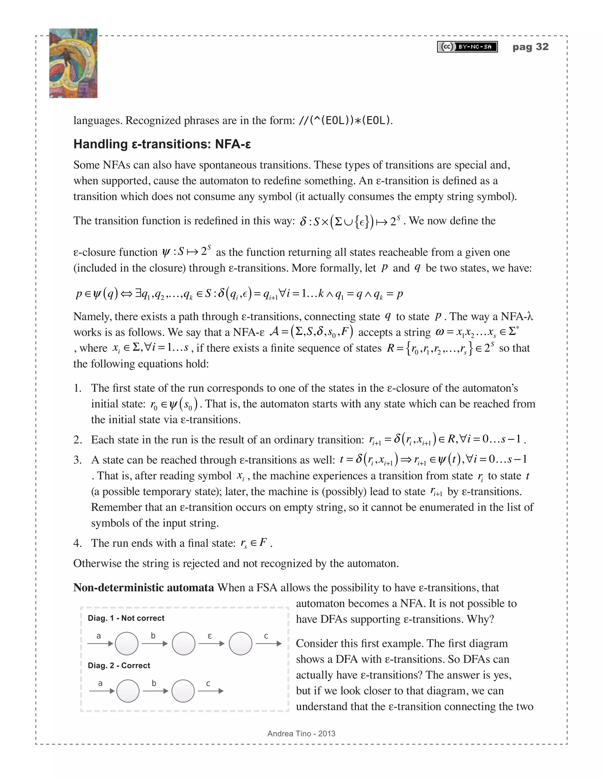
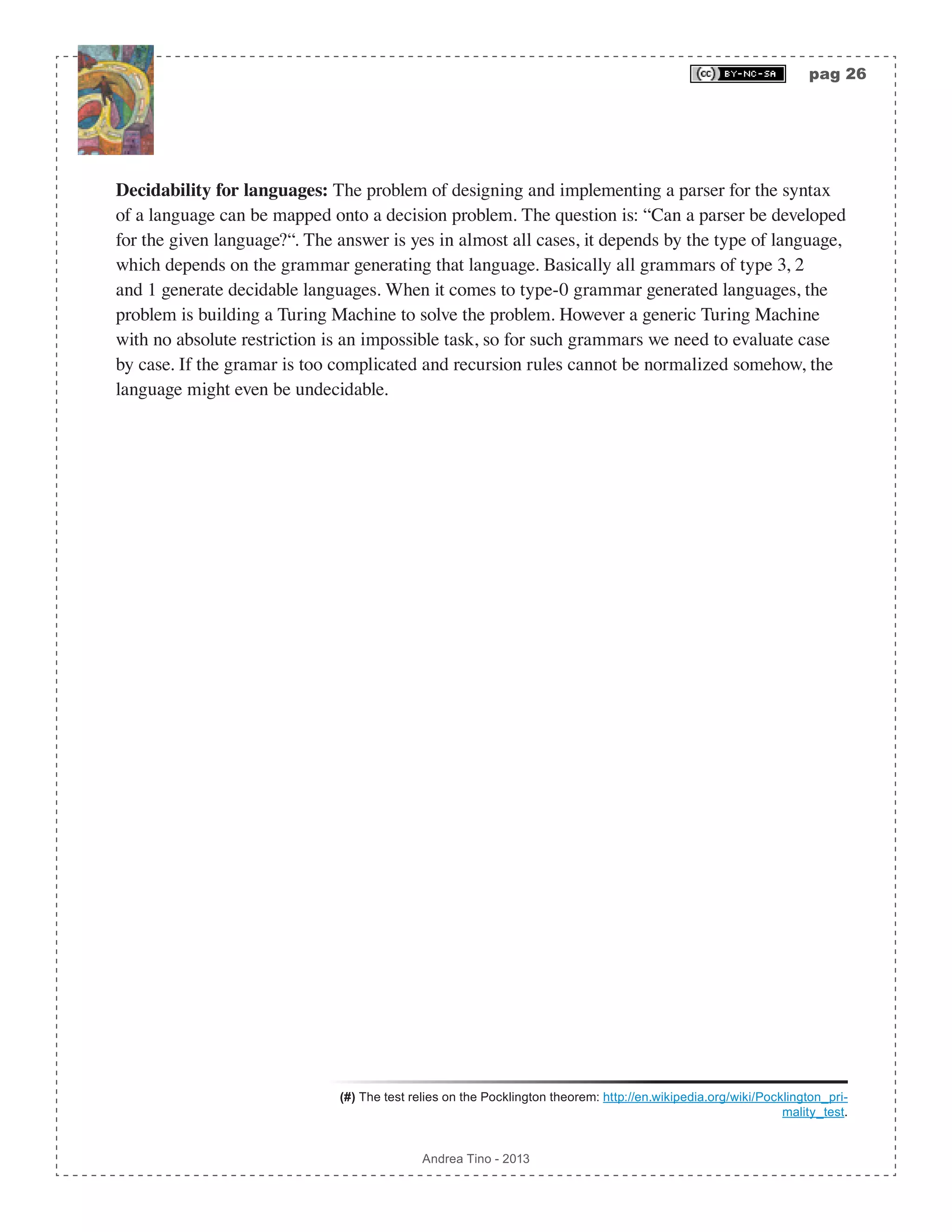
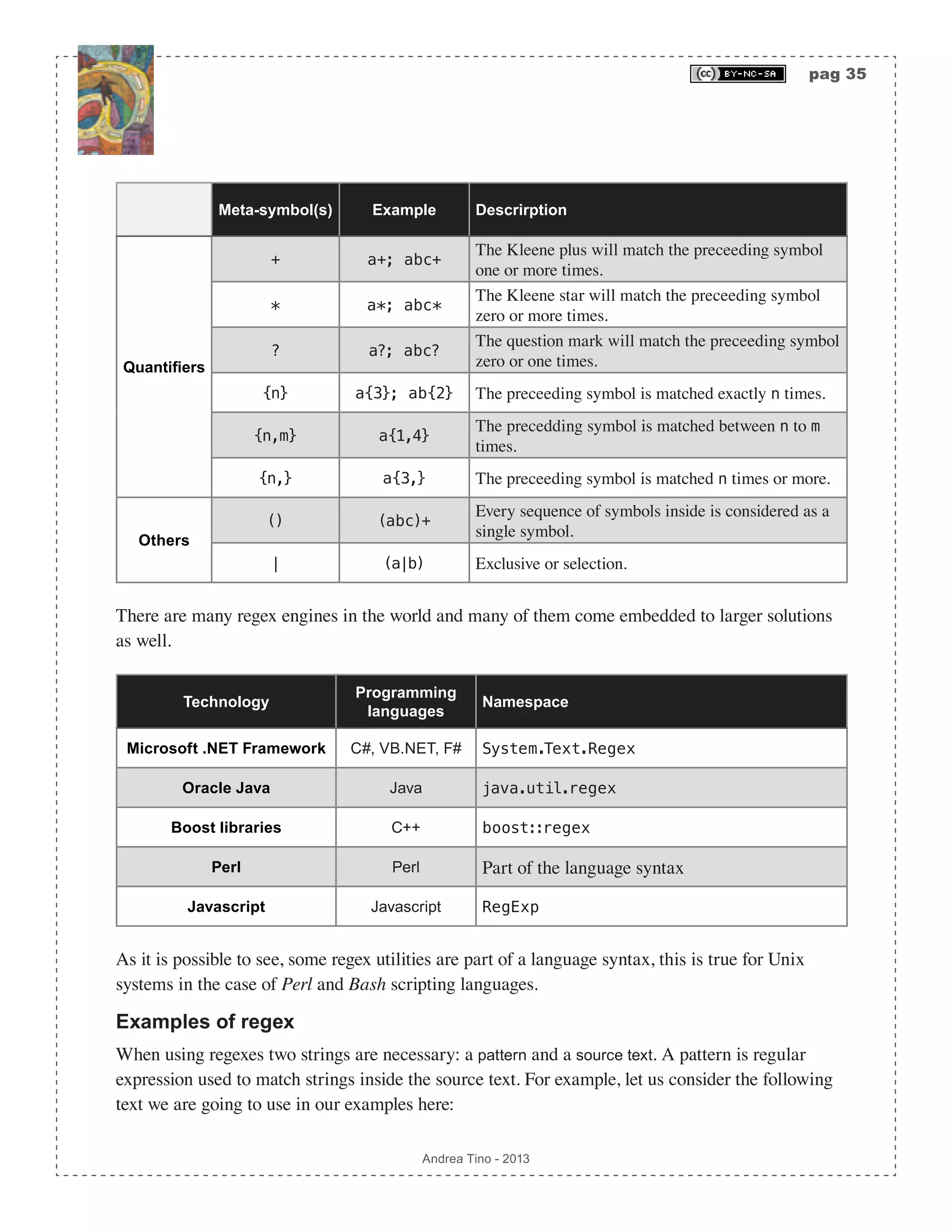
![pag 34 Andrea Tino - 2013 Each symbol in a regexp can by a meta-symbol, thus carrying a special meaning, or a normal symbol with its literal meaning. Although regular expressions can have some variations depending on the system in use, a common specification will be described here. The list of meta-symbols is reported below: R = {., *, +, , {, }, [, ], (, ), ?, ^, $, |}; When we want a regular expression to match a meta-symbol literally, the meta-symbol gets escaped by a special meta-symbol: . What are they used for? Regexp are used to define all words of a language and/or the syntax of a language. Because of this, regexp can be mapped onto FSAs and vice-versa. Furthermore, because regular grammars define a regular language’s syntax, they can be converted into regular expressions and vice-versa. Everything can be summarized by the following property of regexp: regular expressions have the same expressive power as regular gramars. What is a regex? A regexp is a string of characters (of a certain alphabet) and meta-characters that can match a finite or not-finite set of strings on the same alphabet. Character classes Meta-characters in a regular expression are listed in the following table. Each one of them carries a special meaning. Literals are the opposite, they match themselves and carry no special meaning. Meta-symbol(s) Example Descrirption Literals a,b,... hello Every alphabet symbol that is not a meta-symbol is a literal; thus it matches itself. Ranges [ ] [abc] It matches only one single character among those inside the brackets. [^ ] [^abc] It matches one single character that is not listed inside the brackets. - [a-z]; [a-zA-Z] When used inside square brackets, this matches a known range of alphabetical characters and numbers. Classes . f.fox The dot matches all non line-break characters. Anchors ^ ^Fire The caret matches the position before the first character in the string. $ fox$ The dollar matches the position after the last character in the string.](https://image.slidesharecdn.com/creatingacompilerforyourownlanguage-150105162410-conversion-gate01/75/Creating-a-compiler-for-your-own-language-34-2048.jpg)
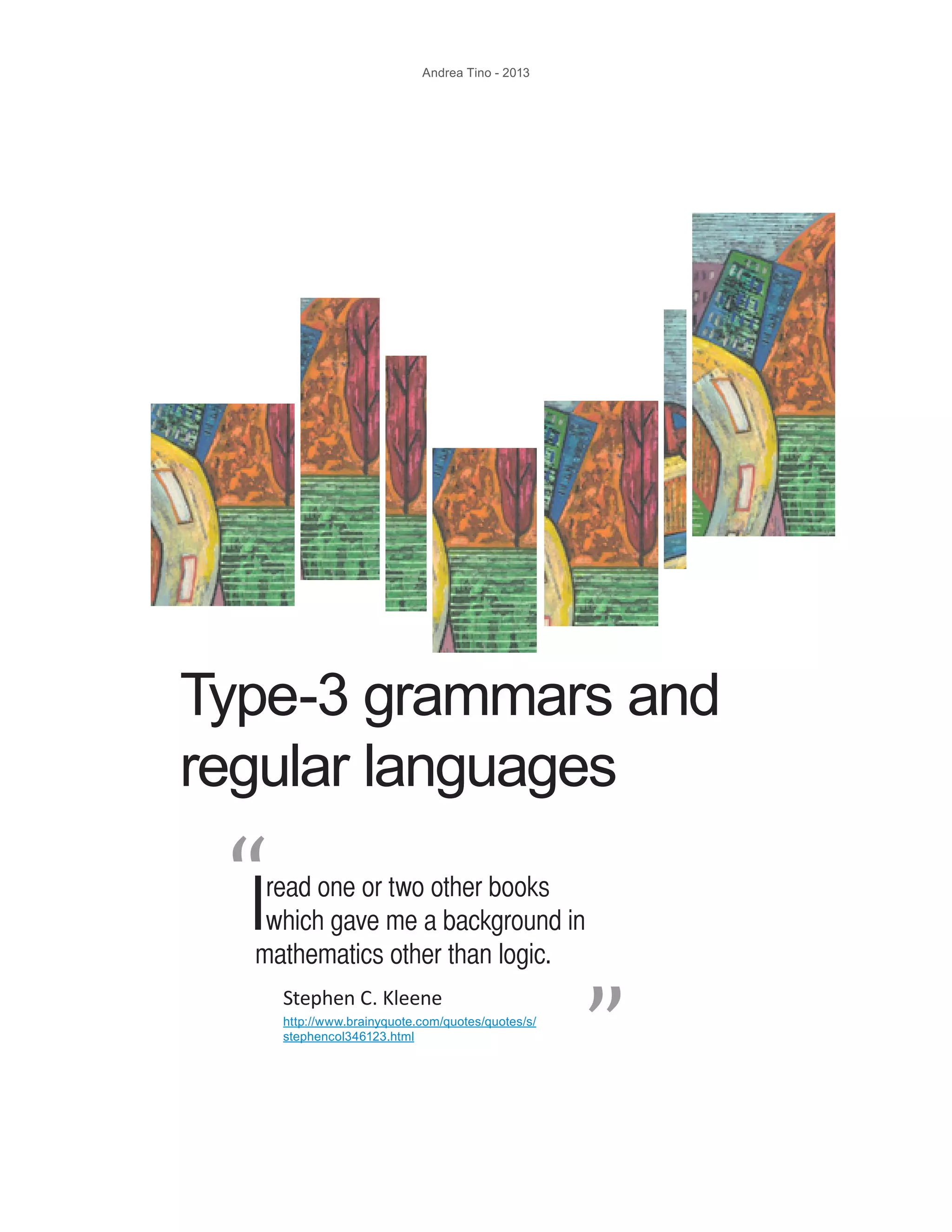
![pag 36 Andrea Tino - 2013 text = “Lorem ipsum dolor sit amet, consectetur adipiscing elit. Fusce 5 vitae fermentum enim. 12 Sed vitae consectetur libero, ac3 hendrerit augue. Cras13 auctor 456 lectus eu lacus455 fringilla, a4 auctor leo 23 euismod.“; Now let us consider the following patterns and let us also consider matched elements. Pattern (Some) Matched text “(L|l).l” “Lorem ipsum dol”, “lor sit amet, consectetur adipiscing el“ “[0-9]+“ “5“, “12“, “456“, “455“, “23” “[a-zA-Z]+“ “Lorem“, “ipsum“, “dolor“, “sit“, “amet“, “consectetur“ “[a-zA-Z]+[0-9]“ “ac3“, “Cras1“, “lacus4“, “a4“ “[0-9][a-zA- Zs]+[0-9]“ “5 vitae fermentum enim. 1“, “3 auctor 4“ These examples show very simple patterns, but it is possible to generate very complex matches. Also, due to the large numbers of regex engines available today, not all patterns always return the same matches. Reported examples should cover the most common functionalities and behave mostly the same for all engines. Regular definitions Regex patterns can become very wide and extremely messy structures as they try to match more complex content. Also it is common to encounter lengthy patterns with identical portions inside them like the following for example: [a-zA-Z]+(a|b|c)[a-zA-Z]*[0-9]?[a-zA-Z]+[0-9]. We find the segment [a-zA-Z] 3 times in the expression and the segment [0-9] 2 times. Considering that they match strings that are common to match (sequences of alphabetical or numeric characters), it would probably be reasonable to use aliases to create references. So let us consider the following regular definitions: char -> [a-zA-Z]; digit -> [0-9]; We can rewrite the previous pattern in a more concise way as: char+(a|b|c) char*digit?char+digit. This also enables reuse, as we can take advantage of the same set of definitions for more patterns. Basic properties Regular expressions, no matter the engine, have important properties. Some of them can be used to](https://image.slidesharecdn.com/creatingacompilerforyourownlanguage-150105162410-conversion-gate01/75/Creating-a-compiler-for-your-own-language-36-2048.jpg)
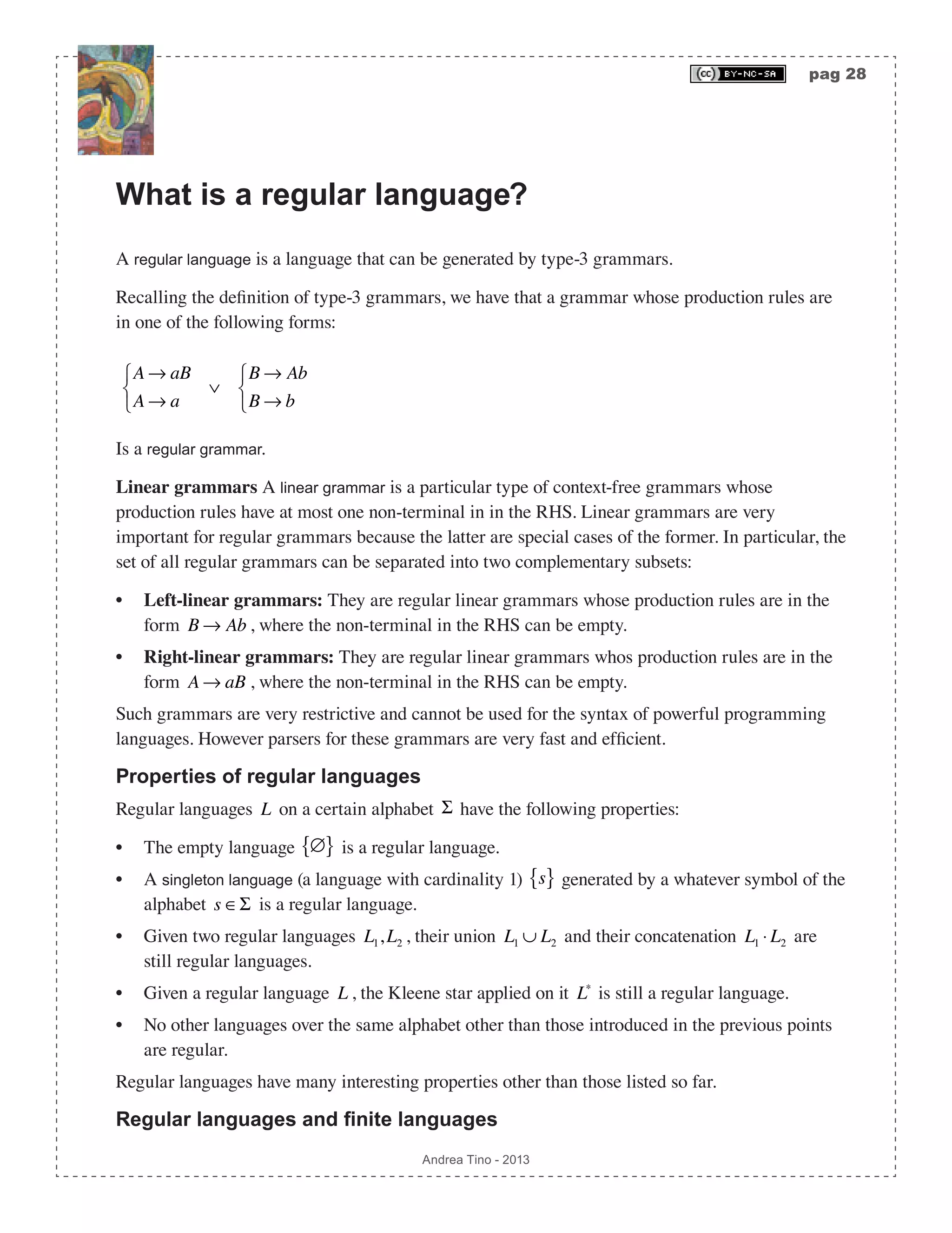
![pag 37 Andrea Tino - 2013 avoid long patterns or to simplify existing ones. • Operator | is commutative: a|b = b|a. • Operator | is associative: (a|b)|c = a|(b|c). • Concatenation is associative: (ab)c = a(bc). • Concatenation is distributive over operator |: a(b|c) = (ab)|(ac), and: (a|b)c = (ac)|(bc). • The empty string ε is concatenation’s identity element: aε = εa = a. • The following equation holds for the Kleene star: a* = (a|ε)*. • The Kleene star is idempotent: a** = a*. From regular expressions to FSAs Regular languages are defined through regular grammars; however regular languages’ grammar can also be defined through regular expressions in a more concise and simpler way. In the Chomsky-Schützenberger hierarchy, type-3 grammars can be parsed by FSAs; now we are going to see how to create a FSA to develop the parser of a regular language. In particular the transformation process will always start from regular expressions. Thompson’s rules There are many methodologies to construct a FSA from a regular expression. [Theo] Regex2FSA: A FSA can always be constructed from a regular expression to create the corresponding language’s parser. The synthesized FSA is a NFA whose states have one or two successors only and a single final state. Among these, Thompson’s rules are a valid option. [Theo] Thompson’s Construction Algorithm (TCA): A NFA can be generated from a regular expression by using Thompson’s rules. TCA is methodology to build a FSA from a regex but not the only one. Some advantages can be considered but this methodology is not the best. • The NFA can be built following very simple rules. • In certain conditions TCA is not the most efficient algorithm to generate the cirresponding](https://image.slidesharecdn.com/creatingacompilerforyourownlanguage-150105162410-conversion-gate01/75/Creating-a-compiler-for-your-own-language-37-2048.jpg)
![pag 38 Andrea Tino - 2013 NFA given a regex. • TCA guarantees that the final NFA has one single initial state and one single final state. TCA’s rules are listed following expressions to be translated. The initial regex is split into different subregexes; the basic rule is considering that a whatever regex maps onto a certain NFA. A generic expression A generic regex s is seen as a NFA N(s) with its own initial state and its own final state. Since TCA generates NFAs having only one initial state and only one final state, the previous assumption is valid. Empty string The empty string expression ε is converted into a NFA where the empty string rules the transition between a state and the final one. Symbol of the input alphabet A symbol a of the input alphabet is converted in a similar way for empty string expressions. The symbol rules the transition between a state and the final one. Union expressions A union expression s|t between two expressions s and t, is converted into the following NFA N(s|t). Epsilon transitions rule the optional paths to N(s) and to N(t). Please note that the union expression is also valid for square bracket expressions [st]. Concatenation expressions When concatenating two expressions s and t into expression st, the resulting NFA N(st) is constructed by simply connecting the final state of the first expression to the initial state of the second one. The final state of the first expression and the initial state of the second one are merged into a single crossing state. s_i s_f N(s) q f ɛ q f a s_i s_f N(s) q f ɛ t_i t_f N(t) ɛ ɛ ɛ](https://image.slidesharecdn.com/creatingacompilerforyourownlanguage-150105162410-conversion-gate01/75/Creating-a-compiler-for-your-own-language-38-2048.jpg)
![pag 39 Andrea Tino - 2013 s_i s_f N(s) s_f t_i N(t) t_f Kleene star expressions When an expression s is decorated with a Kleene star s*, the resulting NFA N(s*) is constructed by adding 4 epsilon transitions. s_i s_f N(s) q f ɛ ɛ ɛ ɛ The final NFA will have a messy shape but it will work as desired. Parenthesized expressions Expressions appearing in parenthesis (s) are converted into the inner expression NFA. So we have that N((s))=N(s). Converting a NFA into a DFA As DFAs are faster than NFAs, very often it can be reasonable to convert a NFA into a DFA to get a more efficient parser for regular languages. This process can sometimes be a little tricky when the NFA being trnsformed has a complex structure. Closures Before diving into the algorithm, the notion of state closure is necessary. [Def] Closure: Given a FSA and one of its states s ∈S , the closure of that state is represented by the set of all states in the automaton that can be reached from it including the original state. The notion of generic closure can be useful, but not as useful as the a-closure’s one. [Def] a-Closure: Given a FSA, a symbol a ∈Σ and one of its states s ∈S , the closure of that state over symbol a is represented by the set of all states in the automaton that can be reached from it through transitions labelled with symbol a including the original state.](https://image.slidesharecdn.com/creatingacompilerforyourownlanguage-150105162410-conversion-gate01/75/Creating-a-compiler-for-your-own-language-39-2048.jpg)
![pag 40 Andrea Tino - 2013 A particular type of a-closure is necessary for pur purposes. [Def] ε-Closure: Given a FSA and one of its states s ∈S , the ε-closure of that state is represented by the set of all states in the automaton that can be reached from it through ε-transitions including the original state. How to get the ε-closure When having a FSA and willing to get the ε-closure of a state, it is possible to follow a simple procedure. 1. The closure set is initially represented by the original state. 2. Each element in the closure set is considered and all transitions from that state are evaluated. If a ε-transition is found, the destination state is added to the set. 3. The previous point is performed everytime until a complete scan of all states in the set causes the closure not to grow. In pseudo-code the algorithm is very simple to define. procedure get_closure(i,δ) set S <- {i}; for ∀s ∊ S do for ∀x ∊ δ(s,ε) do S <- S ∪ {x}; end end The algorithm can be really time consuming considering its complexity is O n2 ( ). Conversion The conversion from a NFA to a DFA is performed in a 2-step process: 1. All ε-transitions are removed. 2. All non-deterministic transitions are removed. Removing ε-transitions Given the original NFA N = Σ,S,δ,s0,F( ), we are going to build a new one ′N = Σ,S, ′δ ,s0, ′F( ) by safely removing all ε-transitions. The final states subset is: ′F = F ∪ s0{ } Ε s0[ ]∩ F ≠ ∅ ′F = F otherwise ⎧ ⎨ ⎪ ⎩⎪ While the transition function is modified so that ε-transitions are removed in a safe way. In particular, for any given symbol s ∈S , we have that all transitions ruled by non epsilon symbols are kept: δ s,a( )= ′δ s,a( ),∀a ∈Σ :a ≠ , while ε-transitions are replaced by more transitions; in particular the following equation holds.](https://image.slidesharecdn.com/creatingacompilerforyourownlanguage-150105162410-conversion-gate01/75/Creating-a-compiler-for-your-own-language-40-2048.jpg)
![pag 41 Andrea Tino - 2013 ′δ s,a( )= δ x,a( ) x∈Ε s[ ] ,∀s ∈S,∀a ∈Σ The trick relies in adding more transitions to replace empty ones. When considering a state and a symbol, new transitions to destination states (labelled with such symbol) are added whenever ε-transitions allow the passage from the original state to destination ones. The result is allowing a direct transition to destination states previously reached by empty connections. Example of ε-transitions removal Let us consider the NFA on the side accepting strings in the form: a*b*c*. The second NFA is the one obtained by removing ε-transitions. To understand how such a result is obtained, let us consider each step of the process. First we consider the final states subset. In the first diagram we have only one final state; however when considering the initial state, we have that its ε-closure contains all other states as well; that’s why we need to make all states as final. We can now consider states and symbols. For example, let us consider couple (s1,b) in the first diagram, the ε-closure of such state is: Ε s1[ ]= s1,s2,s3{ }, by following the definition provided before, we can remove the ε-transition to state s2 and create one transition to s2 labelled with symbol b. Now we consider couple (s2,c) in the first diagram, the ε-closure of such state is: Ε s2[ ]= s2,s3{ }, as before, we can remove the ε-transition to state s3 and create one transition to s3 labelled with symbol c. To understand how transition from s1 to s3 is generated, we need to consider couple (s1,c) and following the same process. The process must be performed for all couples state/symbol; when considering a couple some more states are to be considered. Because of this the process has a complexity equal to: O Σ ⋅ S 2 ( ), which makes the approach lengthy for complex NFAs. NFA integrity Please note that, at the end of the ε-transitions removal process, the resulting NFA is one accepting the same language of the original automaton. The subset construction algorithm After removing ε-transitions, we can proceed removing non-deterministic transitions too from the NFA. We consider a NFA without ε-transitions N = Σ,S,δ,s0,F( ) and transform it into a DFA D = Σ,S D( ) ,δ D( ) ,s0 D( ) ,F D( ) ( ) where: s1 s2 s3 ε ε ca b s3 b c c c a b s2s1 Diag. 2 - Empty transitions removed Diag. 1 - Original NFA](https://image.slidesharecdn.com/creatingacompilerforyourownlanguage-150105162410-conversion-gate01/75/Creating-a-compiler-for-your-own-language-41-2048.jpg)
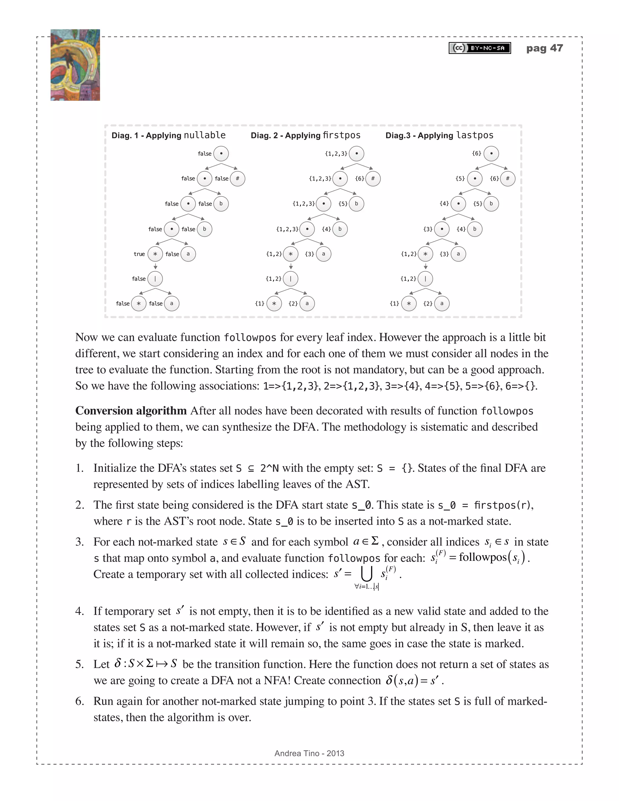
![pag 44 Andrea Tino - 2013 Note that the process at every iteration focuses on a state in the DFA. When focusing on a state, new states are created and outgoing transitions might be created from the state in exam. Direct conversion from a regular expression to a DFA To build a function to directly convert a regex into a DFA, we can first remove empty transitions and then applying the subset construction algorithm. The overall complexity of this operation is O 2S ( ). But instead of a real direct approach, this is a 2-step solution. However a straightforward conversion from a regex to a DFA is possible thanks to another algorithm consisting of 3 steps. 1. AST creation: The AST of an augmented version of the regex is created. 2. AST functions generation: Functions operating on nodes of the AST are synthesized. 3. Conversion: From the AST, by means of the functions as well, the final DFA is generated. Creating the AST Given a regex, we augment it with a special symbol (not part of the regex alphabet) at the end of the same. Once we get the augmented regex, we can draw its AST where intermediate nodes are operators and leaves are alphabet characters or the empty string or the augmentation symbol. The augmenting symbol, here, will be character #, and it is to be applied as the last operator in the original regex pattern. For example, given regex ab*(c|d)+, the augmented regex will be: (ab*(c|d)+)#. The augmentation symbol acts like a normal regex character class symbol and must be concatenated to the whole original regex; that’s why sometimes it is necessary to use parentheses. However parentheses can be avoided in some cases like pattern: [a-zA-Z0-1]*, which simply becomes pattern: [a-zA-Z0-1]*#. One key feature of the tree is assigning numbers to leaves by decorating them with position markers. With this, every leaf of the tree will be assigned an index i ∊ N. The way numbers are assigned to leaves is the one defined by the pre-order depth- traverse algorithm; with the difference that intermediate nodes can be removed by the final list. A corollary of this approach is that the augmentation symbol will always be assigned with the last index. Example of creating an AST out of an augmented regex We consider regex (a|b)*abb. The first step is augmentation, so we get regex (a|b)*abb#. Following operators priority (from lowest to highest priority: |, • and *), we use postfix notation and build the AST. The final step is assigning indices to leaves, the process is simple as we only need to order nodes following the pre-order algorithm to get sequence {a,|,b,*,•,a,•,b,•,b•,#}. From the list we remove AST from augmented regex * • | a b #• • b• * a21 3 5 4 6](https://image.slidesharecdn.com/creatingacompilerforyourownlanguage-150105162410-conversion-gate01/75/Creating-a-compiler-for-your-own-language-44-2048.jpg)
![pag 45 Andrea Tino - 2013 all intermediate nodes: {a,b,a,b,b,#}, so that we can finally assign numbers from left to right as shown in the diagram. Defining AST node functions After building the AST for the augmented regex, some functions are to be defined. Actually it is a matter of defining one function called follopos(i∊N). But to define such a function, 3 more functions are needed. [Def] Function followpos: Given an AST from an augmented regex, function followpos(N):2^N returns the set of all indices following the input index inside the AST. To compute this function, we also define more functions whose behavior is described by the table reported below. Input node n Function firstpos(n) Function lastpos(n) Function nullable(n) The node is a leaf labelled ε {} {} true The node is a leaf with index i {i} {i} false Option node | (S2)(S1) firstpos(s1) ∪ firstpos(s2) lastpos(s1) ∪ lastpos(s2) nullable(s1) OR nullable(s2) Concatenation node · (S2)(S1) if nullable(s1) => firstpos(s1) ∪ firstpos(s2) else => firstpos(s1) if nullable(s2) => lastpos(s1) ∪ lastpos(s2) else => lastpos(s2) nullable(s1) AND nullable(s2) Kleene star node * (S1) firstpos(s1) lastpos(s1) true As it is possible to see, all functions accept a node and return a set of leaf indices, except function nullable which returns a boolean value. Furthermore, a key difference is to be underlined](https://image.slidesharecdn.com/creatingacompilerforyourownlanguage-150105162410-conversion-gate01/75/Creating-a-compiler-for-your-own-language-45-2048.jpg)
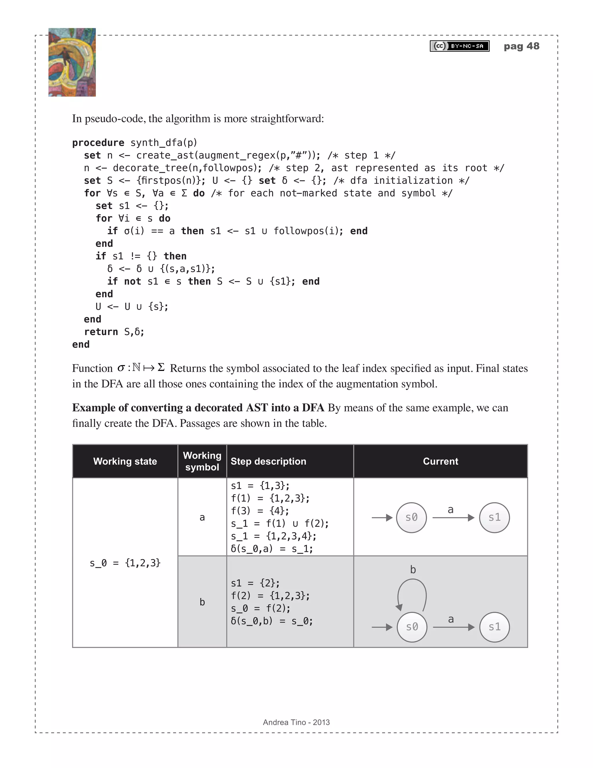
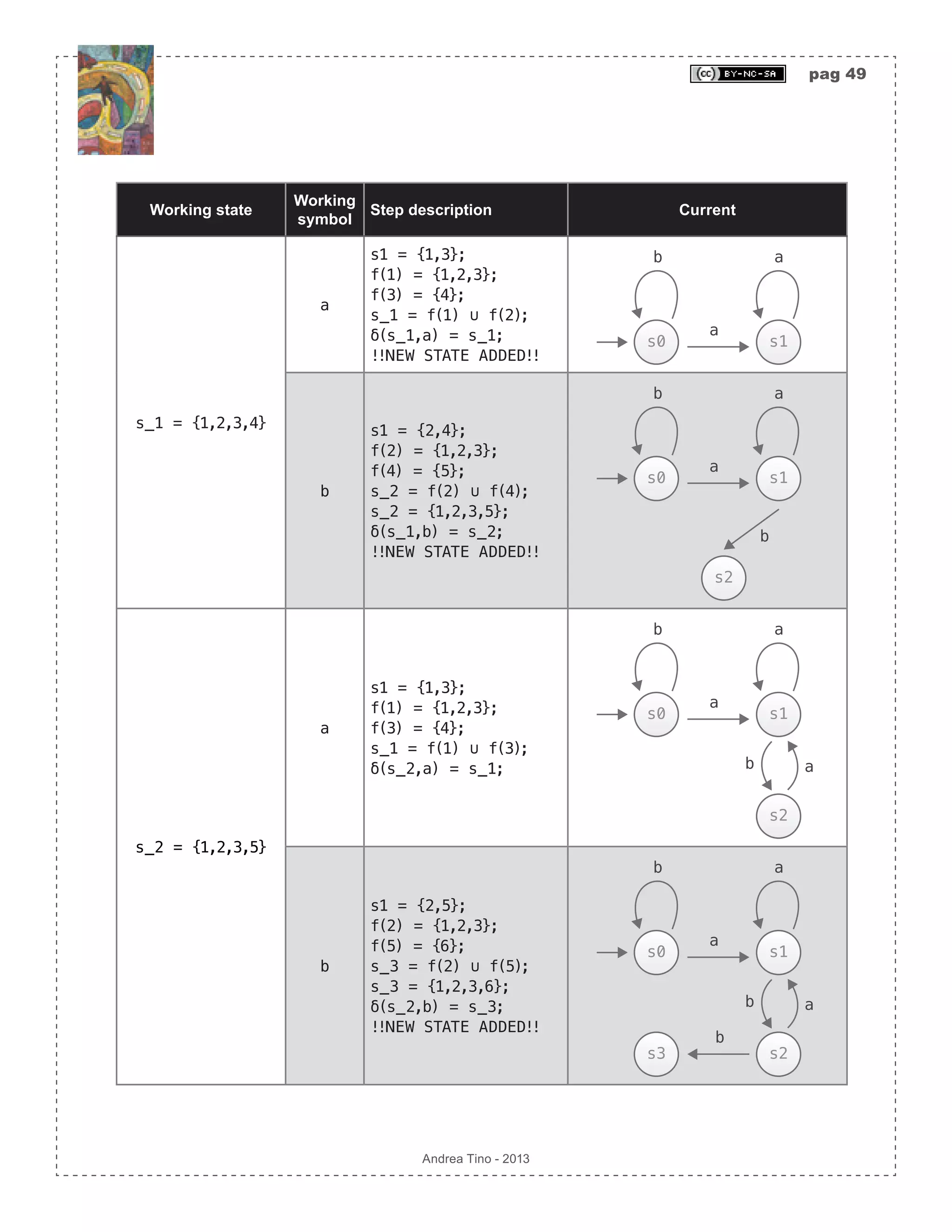
![pag 50 Andrea Tino - 2013 Working state Working symbol Step description Current s_3 = {1,2,3,6} a s1 = {1,3}; f(1) = {1,2,3}; f(3) = {4}; s_1 = f(1) ∪ f(3); δ(s_3,a) = s_1; !!FINAL STATE ADDED!! b a s0 s1 a s2 b a s3 b a b s1 = {2}; f(2) = {1,2,3}; s_0 = f(2); δ(s_3,b) = s_0; b a s0 s1 a s2 b a b a b s3 In the last passage, final states are defined! As we can see, the final automaton is a deterministic one. The approach allows the direct calculation of the DFA from a regex. Minimizing FSAs A question naturally arises: “Is the automaton in minimal form?“. Minimization is a term used to refer to DFAs which have the minimum number of states to accept a certain language. More DFAs can accept the same language, but there is one (without considering states labelling) that can accept the language with the minimum number of states: that DFA is the minimal DFA. When having a DFA, we can try to make it minimal using a sistematic methodology, if final result is the same, then the original DFA was already in its minimal form. [Theo] Minimal DFA existance: For each regular language that can be accepted by a](https://image.slidesharecdn.com/creatingacompilerforyourownlanguage-150105162410-conversion-gate01/75/Creating-a-compiler-for-your-own-language-50-2048.jpg)
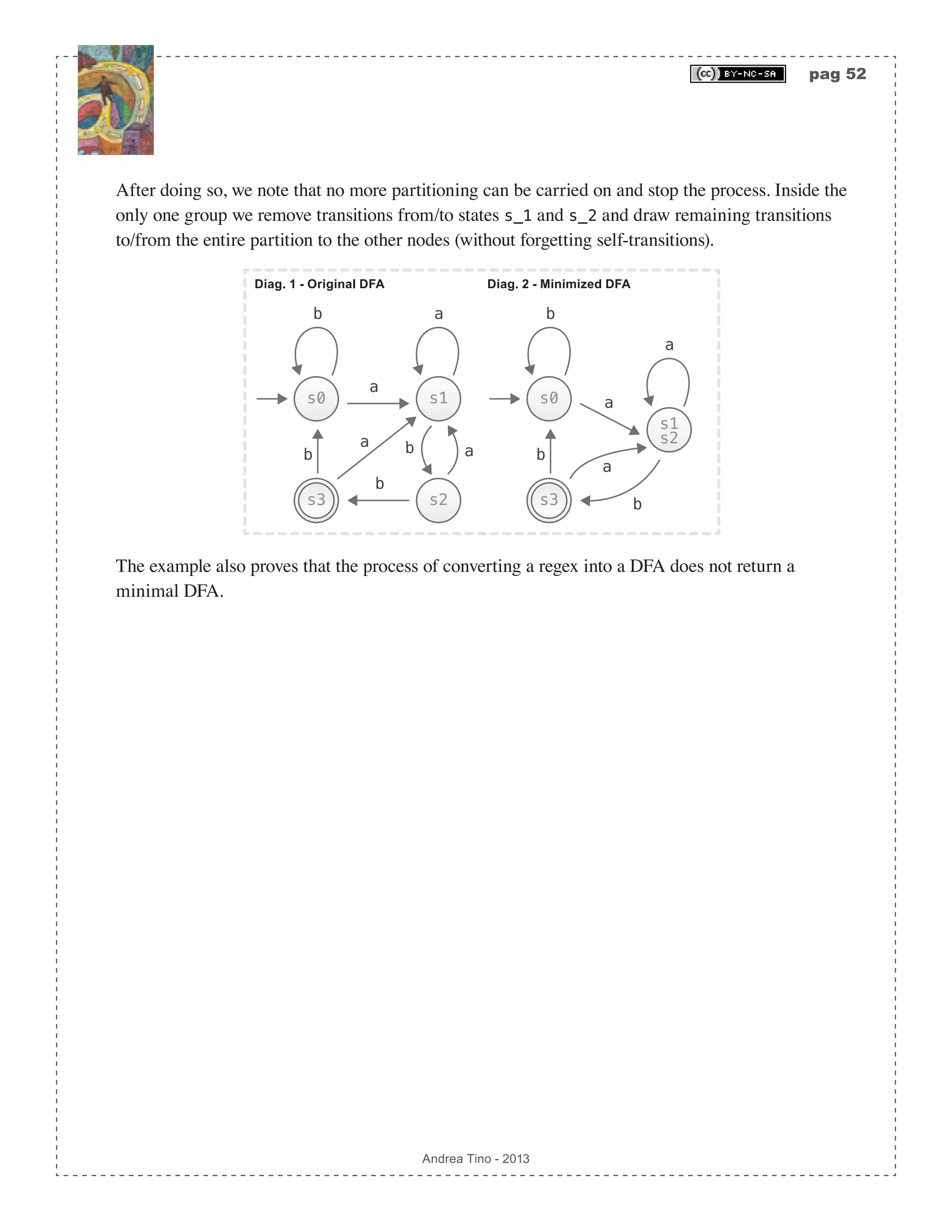
![pag 51 Andrea Tino - 2013 DFA, there exists a minimal automaton (thus a DFA with minimum number of states) which is unique (except that states can be given different names). [Cor] Minimal DFA’s computational cost: The minimal DFA ensures minimal computational cost for a regular language parsing. Hopcroft’s DFA minimization algorithm DFA minimization can be carried out using different procedures; a very common approach is Hopcroft’s algorithm. Considering a DFA, to obtain the minimal form the following procedure is to be applied: 1. Consider the states set S ⊆ , and split it into two complementar sets: the set of final states S F( ) ⊂ S and the set of non-final states S N( ) ⊂ S . 2. Consider a generic group and create partitions inside that group. The rule to create partitions is having all states inside it having the minimal relation property. 3. Proceed creating more partitions until no more partitions can be created. 4. At the end of the partitioning process, consider all partitions to be the new states of the minimized DFA. Remove internal transitions (inside every partition) and leave all partition- crossing transitions. 5. Make the initial state of the minimal DFA the state containing the initial state of the original DFA. Make final states in the minimal DFA all states containing final states in the original DFA. Inside a partition, all states have the following property: [Theo] State in partition: In a minimal DFA, a state in a partition has at least one transition to another state of the same partition. A direct consequence of the previous result, is a useful approach to locate partitions, or better to locate states that can be removed from a partition in order to be placed into a different one. [Cor] State not in partition: During the partitioning process to get the minimal DFA from a DFA, a state is to be placed into a different partition when it has no transitions to states of that partition. Example of DFA minimization We consider the previous example and try to check whether the DFA is a minimal one or not. By carrying out the partitioning process, we note that state s_0 falls inside the non-final states partition. We also note that in that partition, no transition are directed to s_0 from other states in the group: state s_0 is to be placed into a different partition.](https://image.slidesharecdn.com/creatingacompilerforyourownlanguage-150105162410-conversion-gate01/75/Creating-a-compiler-for-your-own-language-51-2048.jpg)

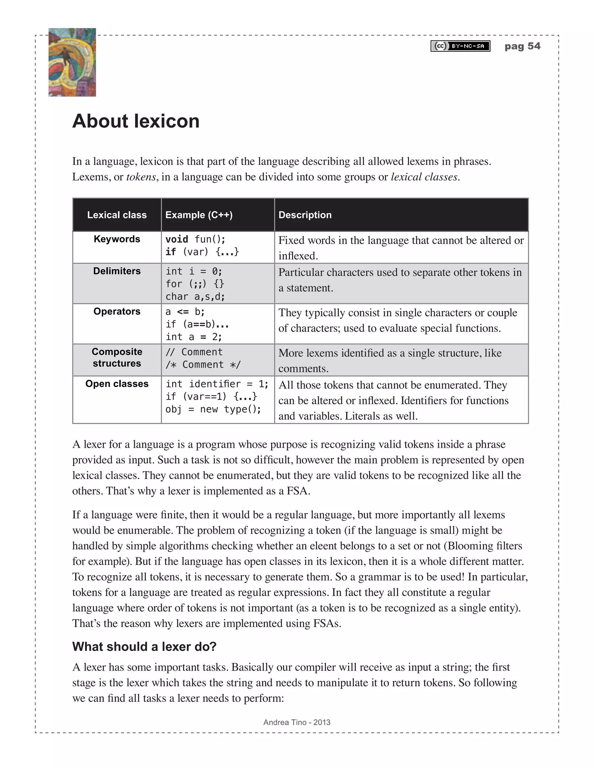
![pag 55 Andrea Tino - 2013 • A lexer must provide a system to isolate low level structures from higher level ones representing the syntax of the language. • A lexer must subdivide the input string in tokens. The operation is known as tokenization and it represents the most important activity carried out by a lexical analyzer. During this process, invalid sequences might be recognized and reported. • A lexer is also responsible for cleaning the input code. For example white spaces are to be removed as well as line breaks or comments. • A lexer can also perform some little activities concerning the semantic level. Although semantics is handled as the final stage of the compilation process, lexers and parsers can provide a little semantic analysis to make the whole process faster. A typical application, is having lexers insert symbols and values in the symbol table when encountering expressions like variables. Separation is not compulsory It is important to underline a concept. Lexical analysis and syntax analysis can be carried out together into the same component. There is no need to have two components handling lexicon and syntax separately. If a compiler is designed as modular, it is easier to modify it when the language changes. Communications between lexer and parser We will consider a compiler with a modular structure, so the lexer and the parser in our compiler are implemented as two different components. However they interact together. In particular, the parser requests one token at a time to the lexer which provides them. The source code is not seen by the parser, as it comes as input to the lexer. About tokens There a little of naming to understand when considering one language’s lexicon. The first thing to understand is the difference between a lexem and a token in the language. [Def] Lexem: In a language, a lexem is the most basic lexical constituent. A lexem is represented by a word of the language carrying, at most, one single semantic value. [Def] Token: In a language, a token is a lexem or a sequence of lexems. It is the unit of information carrying a certain semantic value which is returned by the lexer to the parser. The difference os not that evident and not so simple to grasp. However that’s when examples come to the rescue. An identifier is a lexem and at the same time a token for example. A keyword is another example of lexem being a token as well. On the other hand, a comment like /* comment */ in C++, is a token, but it is a sequence of different lexems tarting from comment delimiters /* and */. An easy way to differentiate tokens from lexems is placing our point of view right in between the lexer and the parser. Everything which the lexer passes to the parser is a token. If a](https://image.slidesharecdn.com/creatingacompilerforyourownlanguage-150105162410-conversion-gate01/75/Creating-a-compiler-for-your-own-language-55-2048.jpg)
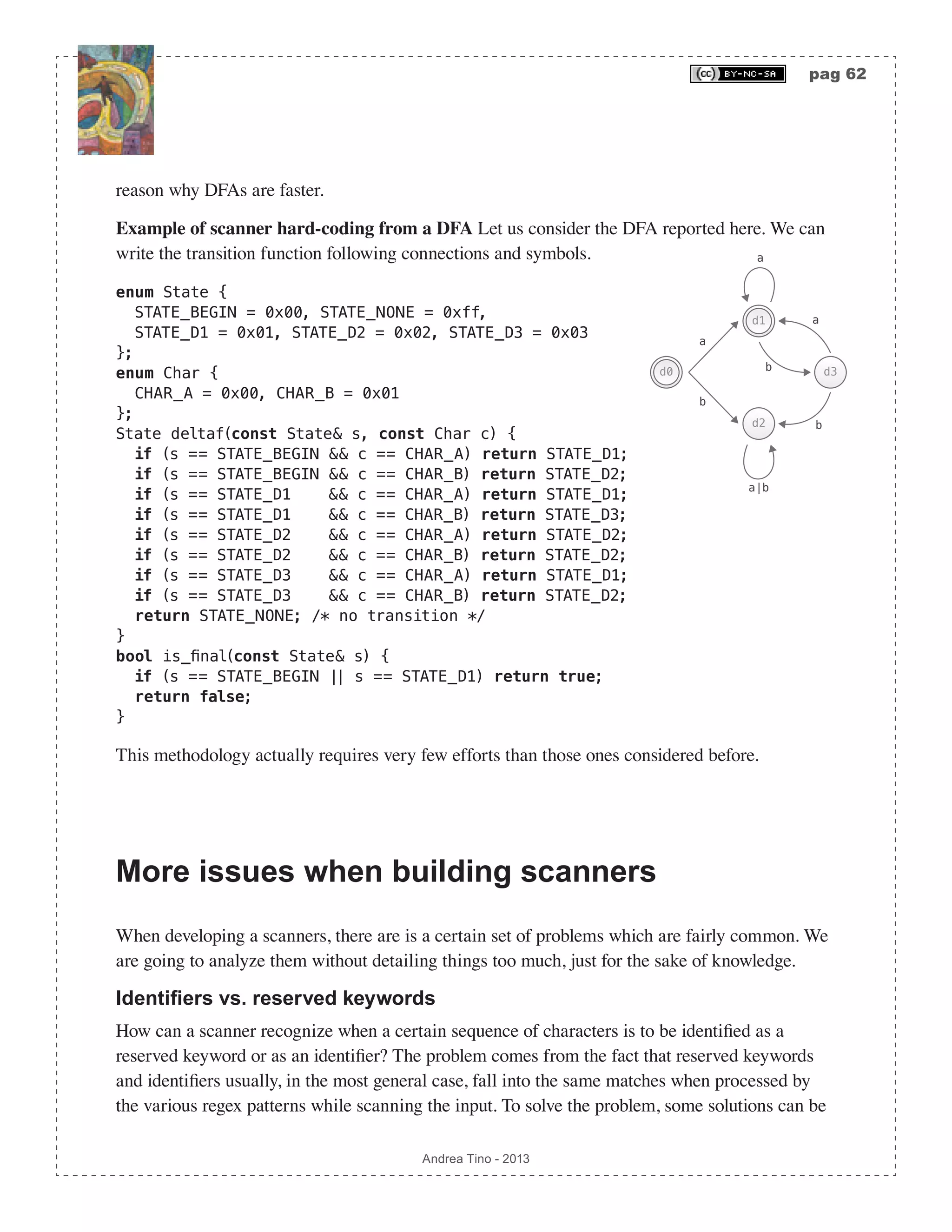
![pag 58 Andrea Tino - 2013 In this case as well, only union, concatenation and Kleene-star characters are considered. Every other regex character is to be converted into a more basic form using the afore-mentioned regex symbols. For example regex a(a|b)+ should be converted into a(a|b)(a|b)*. Example of scnner hard-coding from a regex The problem of this approach is the order of operators. Although not necessary, one should figure out about the operators tree, after that, starting from the root, rules are applied. Consider the following example for regex (a(a|b)*)|b. enum Char { CHAR_A = 0x00, /* in alphabet: a */ CHAR_B = 0x01 /* in alphabet: b */ }; Char cur(const std::string& str, idx i) { if (i >= str.length() || i < 0) throw std::exception(); if (str[i] == ‘a‘) return CHAR_A; if (str[i] == ‘b‘) return CHAR_A; } bool scanner(const std::string& input) { /* the scanning function */ idx i = 0; try { if (cur(input,i) == CHAR_A) { /* test */ i++; /* consume */ while (cur(input,i) == CHAR_A || cur(input,i) == CHAR_B) /* kleene */ i++; /* consume */ return true; /* accept */ } else if (c == CHAR_B) return true; /* test */ return false; /* reject */ } catch (std::sxception e) { return false; /* reject */ } } The code above implements a scanner recognizing the provided regex. Be careful about the fact for which the procedure will implement a scanner for a unique regex only. If another regex is to be matched, a new procedure must be written. To use the scanner, the main routine is to be simply written and function scanner to be called inside it. Procedural approach: regular grammar 2 program When having a grammar, it is possible to write a scanner from that. As for regexes, a methodology can be considered to create the scanning program. This time, rules focus on production rules of the grammar to synthesize the scanner. The scanner function will have the same structure and interface from the previous approach. Also, function cur and enum Char are recycled as well. Rules Procedural code is added according to non-terminals and produnction rules in the grammar.](https://image.slidesharecdn.com/creatingacompilerforyourownlanguage-150105162410-conversion-gate01/75/Creating-a-compiler-for-your-own-language-58-2048.jpg)
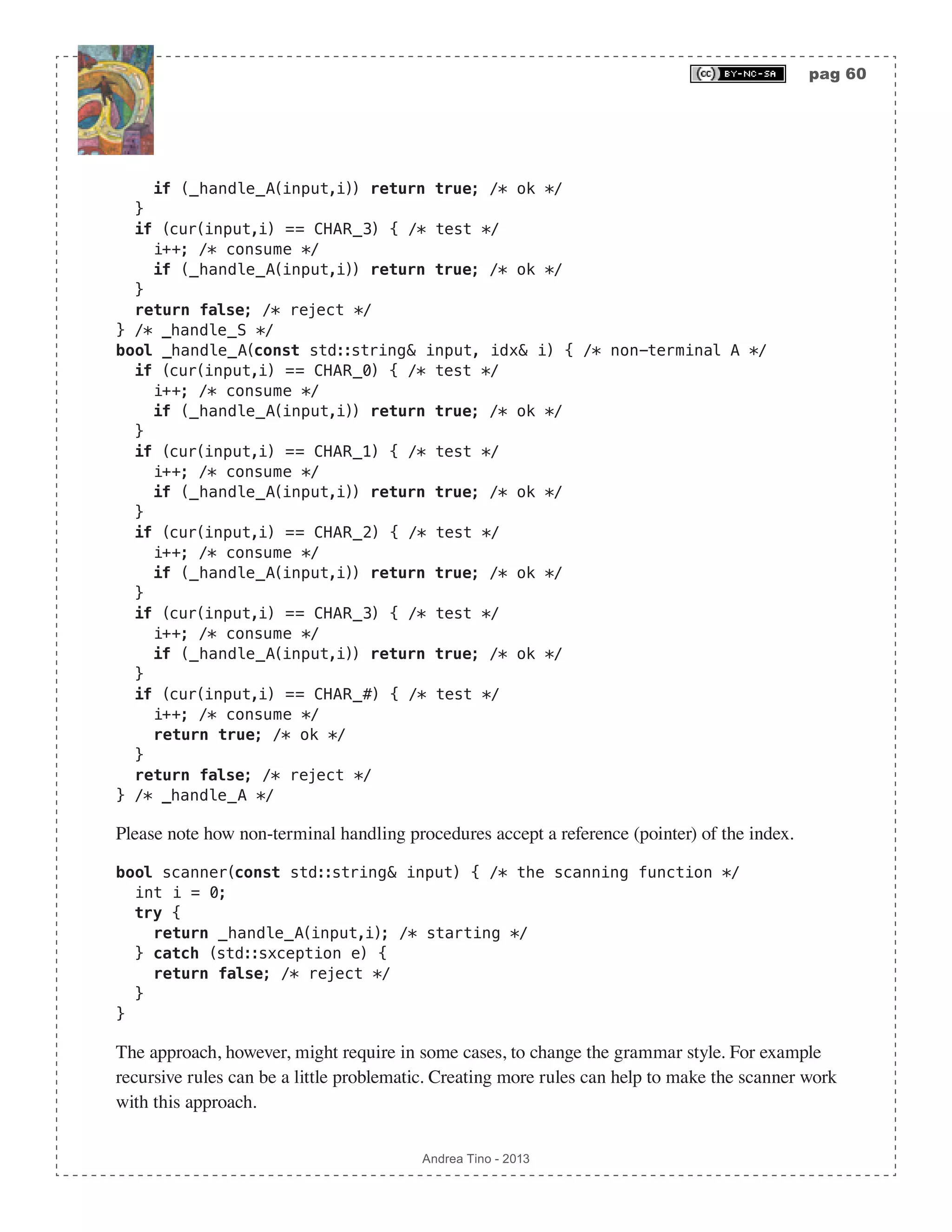
![pag 59 Andrea Tino - 2013 1. Write a function for each non-terminal. 2. Write a test for each alternative in the production rule for each production rule. 3. Call corresponding functions for each non-terminal appearing as RHS in production rules. 4. Place return points in all places where a grammar rule is to be verified and when terminals are reached. First, all non-terminals appearing in rules are to be processed and functions are to be created accordingly. After that, one focuses on production rules. For each production rule alternatives are to be evaluated. For each alternative a test is written. In the end, every alternative’s RHS is evaluated and functions called when the corresponding non-terminal is encountered. Example of scanner hard-coding from a regular grammar Consider the following regular grammar: L = {S,A,0,1,2,3,#}; V = {S,A}; T = {0,1,2,3,#}; S -> 0 A | 1 A | 2 A | 3 A; A -> 0 A | 1 A | 2 A | 3 A | #; The code to synthesize is shown below. The enumeration will now host terminal and non-terminal symbols, while function cur will act accordingly: enum Char { /* terminals only */ CHAR_0 = 0x00, CHAR_1 = 0x01, CHAR_2 = 0x02, CHAR_3 = 0x03, CHAR_S = 0xf0 }; Char cur(const std::string& str, idx i) { if (i >= str.length() || i < 0) throw std::exception(); if (str[i]==‘0‘) return CHAR_0; if (str[i]==‘1‘) return CHAR_1; if (str[i]==‘2‘) return CHAR_2; if (str[i]==‘3‘) return CHAR_3; if (str[i]==‘#‘) return CHAR_S; } Before handling function scanner, we need to create all functions to manage with non-terminals: bool _handle_S(const std::string& input, idx& i) { /* non-terminal S */ if (cur(input,i) == CHAR_0) { /* test */ i++; /* consume */ if (_handle_A(input,i)) return true; /* ok */ } if (cur(input,i) == CHAR_1) { /* test */ i++; /* consume */ if (_handle_A(input,i)) return true; /* ok */ } if (cur(input,i) == CHAR_2) { /* test */ i++; /* consume */](https://image.slidesharecdn.com/creatingacompilerforyourownlanguage-150105162410-conversion-gate01/75/Creating-a-compiler-for-your-own-language-59-2048.jpg)
![pag 75 Andrea Tino - 2013 Different parsing methodologies Parser can process input using two main approaches: • Top-down parsing: Parsing is conducted starting from the root of derivations subtrees and proceeding to leaves. Rules are picked and tested, if a rule fails matching a string, backtracking ensures recovery to the latest good position in the tree. The direct consequence of this approach is that ASTs are built starting from the root down to leaves. • Bottom-up parsing: Parsing is performed starting from leaves of derivation subtree up to the root. Concepts of shifting and reduction are needed as well as a stack to store sequences of symbols possibly matching a rule. It is possible to develop the parser using a state machine. The direct consequence of this approach is that ASTs are built starting from the leaves up to the root. So far we put much focus onto bottom-up parsers because they are very efficient and common today. However we will also see, later, how top-down parsers are structured, but a deeper analysis will be conducted on bottom-up parsers anyway. Classification today Parsing algorithms are today divided into some categories depending on the following parameters: • Derivation policy: Parsers can be LeftMost or RightMost. • Parsing direction: Which is the direction of the prsing process? This is a parameters depending on how sequences of tokens are handled. If the approach starts from the root of derivations, then we have LeftToRight parsers, these parsers are TopDown parsers as a direct consequence. If the parsing algorithm starts from leaves of derivations in order to proceed to the root, then we have RightToLeft parsers, these parsers are BottomUp parsers as a direct consequence. • Lookahead characters: Parsers can take advantage of a lookahead character. It means that before actions take place on the sequence of tokens/symbols loaded so far, the parser can request some tokens to peek what is next; however these lookahead symbols will not be part of current actions. The more lookahead symbols are used, the more predictive the parser can be; however this number must be small, if not the parser will not be efficient. The bottom-up parsing algorithm described before, for example, is a parsing algorithm that took advantage of one lookahead symbol. Basing on parameters introduced so far, parsersing algorithms are today classified using the following scheme: <Direction><Derivation><Lookahead>, thus: (L|R)(L|R)[k]. Very common algorithms are: • LL parsers: They are LeftToRight LeftMost top-down parsers using one lookahead character.](https://image.slidesharecdn.com/creatingacompilerforyourownlanguage-150105162410-conversion-gate01/75/Creating-a-compiler-for-your-own-language-75-2048.jpg)
![pag 80 Andrea Tino - 2013 Overview Top-down parsers proceed creating the AST starting from the root to the leaves. The class of parsing algorithms used today to implement such parsers is LL(k): LeftToRight LeftMost parsers with k lookahead symbols. LL parsers are not an option, due to the fact that the AST is built from the root to the leaves, the approach is top-down and the parser proceeds from left to right necessarly. Taxonomy of top-down parsers When considering top-down parsers, there are some algorithms to implement them. The Chomsky- Schützenberger hierarchy tells us how to implement such parsers (using pushdown automata), however we can find other approaches rather than going for the most generic one. “Generic“ is probably the best word. In fact the Chomsky-Schützenberger hierarchy considers pushdown automata as the computational structure able to parse a CFG, and so it is! But if our grammars have some restructions, more efficient and fine-tuned algorithms can be considered. Why? Because pushdown automata can be difficult to implement and might require time. Today, top-down parsers can be divided into two groups: Algorithm Efficiency Descrirption Recursive descent They are not efficient; back- tracking features are needed. The grammar also needs to have a particular form. The algorithm considers the input string and tries to descent the derivations tree following possible branches. A lot of attempts might be required depending on the grammar size, backtracking is necessary upon errors, in order to recover and try a different derivation path. Predictive They are efficient. Here as well, grammars need to have a particular form. The algorithm proceeds on derivations having a par- ticular structure as not all grammars can be handled by this methodology. Recursive predictive descent They are efficient. No all gram- mars can be handled by this approach as well. It is a special form of recursive descent parsing, but no backtracking is needed, thus making the process faster and more efficient. Left recursion Recursive descent algorithms (with backtracking or not) have a problem: they operate in way for which left-recursion can make them go infinite loop. What is left-recursion by the way? [Def] Left-recursive grammars: A grammar is said to be left-recursive when it contains](https://image.slidesharecdn.com/creatingacompilerforyourownlanguage-150105162410-conversion-gate01/75/Creating-a-compiler-for-your-own-language-80-2048.jpg)
![pag 81 Andrea Tino - 2013 at least one left-recirsive rule. [Def] Left-recursive rule: Given a CFG, a left-recursive rule is a rule in the form: A ⇒+ Aα , thus the non-terminal in LHS appears as the left-most symbol in the LHS of the same rule. [Def] Immediate left-recursive rule: A left-recursive rule is said to be immediate when the left-recursion shows at one-step distance: A ⇒1 Aα , thus the left-recursion is evident. [Def] Indirect left-recursive rule: Left recursion might not show in rules of a CFG. New rules can be created when processing derivations; if starting from a non-terminal the grammar allows derivation A ⇒∗ Aα to occur, then that grammar is affected by indirect left-recursion. Left-recursion is definitely a problem for top-down parsers. When designing a language and willing to parse it using a top-down parser, the grammar must be designed to avoid left-recursion. If the grammar is affected by left-recursion, methodologies exist to remove it and fix the grammar. Handling immediate left recursion Recognizing immediate left-recursions is very simple as they show themselves in the rules of the grammar. When a non-terminal appear both in LHS and as the left-most symbol in RHS if a rule, then that rule is left-recursive. Simple case How to fix immediate left-recursion? Very easy. Consider left-recursive rule: A -> A α; | A -> β; /* where β != A γ */ Let us replace it with: A -> β B; /* non-terminal B added in the grammar */ B -> α B; B -> ε; /* from left-recursion to right-recursion */ As it is possible to see, the recursion is moved from left to right, a new equivalent grammar is created. The procedure does not remove a recursion as such a process is impossible. A recursive rule will remain recursive. However right recursion is ok as it can be handled by top-down parsers. Also please not how a non-terminal is inserted in the grammar together with the empty string terminal (if it was not part of the grammar originally). General case In the most general case, a left-recursive rule in the form: A ⇒ Aα1 | Aα2 || Aαm | β1 | β2 || βn βi ≠ Aγ ,γ ∈ V ∪T( )∗](https://image.slidesharecdn.com/creatingacompilerforyourownlanguage-150105162410-conversion-gate01/75/Creating-a-compiler-for-your-own-language-81-2048.jpg)
![pag 83 Andrea Tino - 2013 procedure rem_ilrec(V,T,P) /* grammar as input */ precond: V = {A1,A2...An}; for i = 1..n do for j = 1..i-1 do P = P - {Ai -> Aj γ}; P = P ∪ {Ai -> α γ} ∀α : Aj -> α; end rem_lrec(); /* handles immediate left-rec */ end end Example Let us consider the following grammar affected by indirect left-recursion: T = {a,b,c,d,f}; V = {S,A}; S -> A a; S -> b; A -> A c; A -> S d; A -> f; 1. We first sort non-terminals: S, A. 2. We consider non-terminal S. In the sequence it is the first, no one preceding it. Nothing to do aside from checking for immediate left-recursions. No immediate left-recursion. 3. We now consider non terminal A and locate rules having A as LHS and one non-terminal precending A in the sorting (S only) as the left-most symbol in RHS. We have only one rule matching: A -> S d. We replace this rule with A -> b d, A -> A a d rules. So final rules for A will be: A -> A c, A -> A a d, A -> b d and A -> f. Some of them are affected by immediate left-recursion, so we fix them into: A -> b d B, A -> f B, B -> c B, B -> a d B and B -> ε. Left factorization If we want to use a top-down parser to handle a grammar, we must make that grammar a non-left- recursive one. However if we also wish to use a predictive algorithm (the most efficient one), we also need to be sure that grammar is left-factored as well. Left-factorization is deeply connected to the concept of predictive grammar. A grammar must be predictive to be handled by a predictive parsing algorithm. [Theo] Predictive gramars: A top-down predictive parsing algorithm cannot handle non-predictive grammars. [Theo] Predictive and left-factorized grammars: A left-factorized grammar is also a predictive grammar. What is left-factorization? Consider the following production rule for a dummy grammar (YACC notation):](https://image.slidesharecdn.com/creatingacompilerforyourownlanguage-150105162410-conversion-gate01/75/Creating-a-compiler-for-your-own-language-83-2048.jpg)
![pag 85 Andrea Tino - 2013 The grammar is predictive (left-factorized). Also note how new non-terminals are added to the original grammar. This approach makes the grammar getting bigger. Non-left-recursive grammars A result is obvious: [Lem] Predictive and non-left-recursive grammars: All predictive grammars are not affected by left recursion. And is very simple to prove as the left-factorization process considers the left-recursion removal as part of its steps. LL(1) grammars LL parsers are used as today’s mean to handle (particular types of) CFGs. However we could see that some algorithms can be used to develop a LL parser. Two are the most important: • Predictive: They take advantage of parsing tables. • Predictive recursive descent: They are a subclass of recursive descent algorithms, but no backtracking is used. As well as recursive descent, predictive recursive descent take advantage of recursive functions. Simple recursive descent algorithms involve backtracking and recursive functions and are not used as real implementations. That’s why we will not cover them here. [Def] LL grammars: LL grammars are a particular subset of CFG grammars that can be parsed by LL(k) parsing algorithms. LL grammars and predictiveness To handle a grammar using a top-down generic parser, that grammar must be non-left-recursive. When we want to use predictive approaches (more andvanced and efficient) we need to have predictive grammars. Detailing LL(1) grammars As specified before, LL(1) parsers are LL parsers using 1 lookahead token only. [Def] LL(1) grammars: LL(1) grammars are grammars that can be parsed by LL(1) parsing algorithms.](https://image.slidesharecdn.com/creatingacompilerforyourownlanguage-150105162410-conversion-gate01/75/Creating-a-compiler-for-your-own-language-85-2048.jpg)
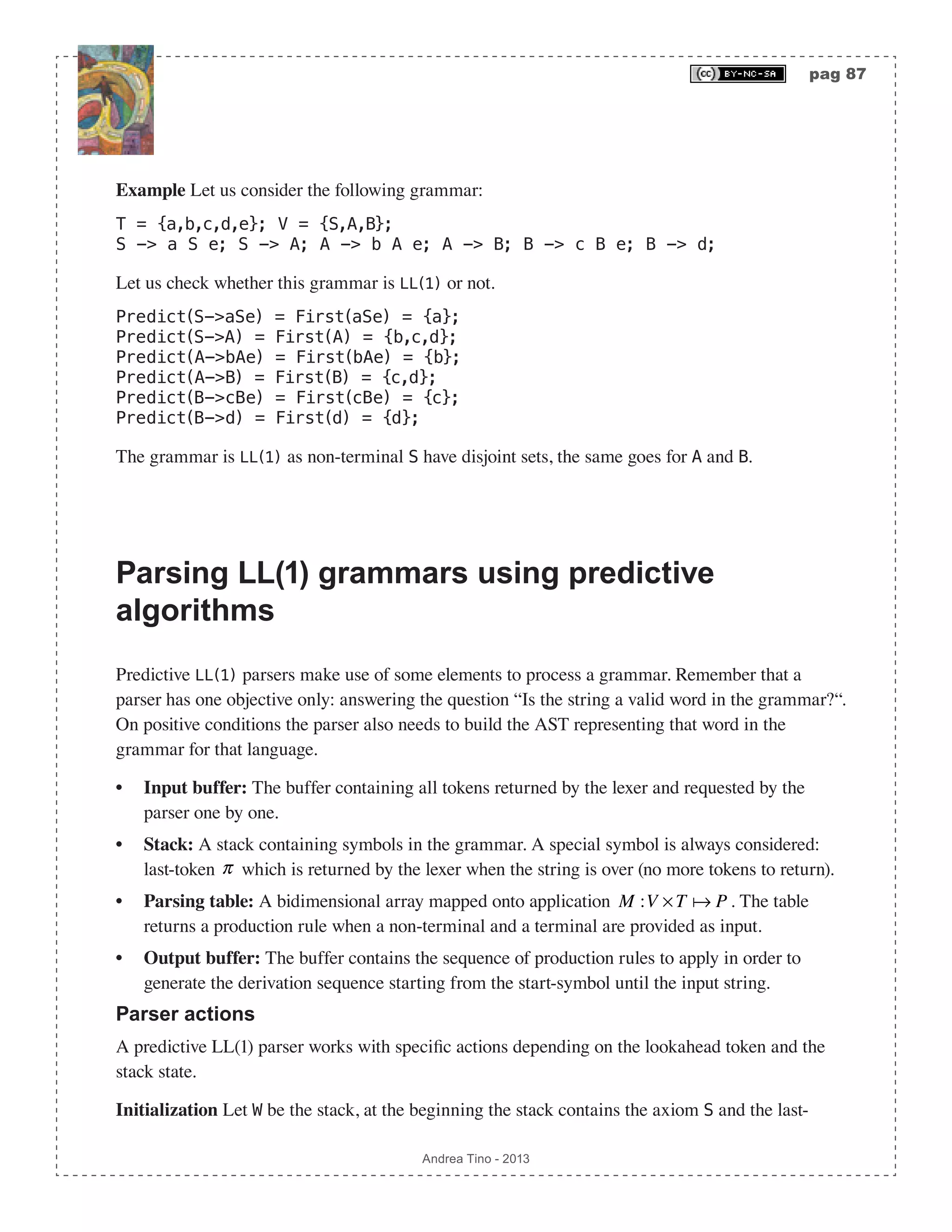
![pag 86 Andrea Tino - 2013 These types of grammars can be easily parsed. Having one lookahed symbol can make the whole process more efficient than when using more lookahead tokens sometimes. Also, LL(1) parsers are very easy to implement. The concept of predict When handling LL(1) grammars, there is an important quantity that can be really helpful to solve the decision problem: “Is a certain grammar a LL(1) grammar?“. This entity is called predict of a production rule. [Def] Predict-set: Let G V,T,P,S( ) be a CFG and p ∈P a production rule in the form p : A ⇒α . The predict-set of p , written as Predict p( ), is the set containing all look- ahead tokens (terminals), usable by a LL(1) parser, indicating that production rule p is to be applied. Calculating the predict-set The predict-set for generic rule A ⇒α can easily be evaluated using the following rule: Predict A ⇒α( )= First α( ) /∃α ⇒∗ First α( )∪ Follow A( ) ∃α ⇒∗ ⎧ ⎨ ⎪ ⎩ ⎪ Example Let us consider the following grammar: T = {a,b,c,ε}; V = {S,A,B}; S -> A B c; A -> a; A -> ε; B -> b; B -> ε; Let us calculate some predict-sets: Predict(S->ABc) = First(ABc) = {a,b,c,ε}; Predict(A->a) = First(a) = {a}; Predict(A->ε) = First(ε) ∪ Follow(A) = {b,ε}; Predict(B->b) = First(b) = {b}; Predict(B->ε) = First(ε) ∪ Follow(B) = {c,ε}; Conditions for a grammar to be LL(1) Predicts are really helpful when some facts on LL(1) grammars are to be considered. A particualr handy result is the following: [Theo] Predict-set: A CFG is LL(1) if and only if predict-sets for all production rules having the same LHS are disjoint; for all non-terminals. The theorem is anecessary and sufficient condition, so a very useful tool.](https://image.slidesharecdn.com/creatingacompilerforyourownlanguage-150105162410-conversion-gate01/75/Creating-a-compiler-for-your-own-language-86-2048.jpg)
![pag 90 Andrea Tino - 2013 2. If the empty-string symbol belongs to the first-set of RHS of rule A ⇒α , then add that production to M A,a( ) for every terminal which belongs to the follow-set of the rule’s LHS: ∈First α( )⇒ M A,a( ) ⊇ A ⇒α{ },∀a ∈Follow A( ). 3. If the empty-string symbol belongs to the first-set of RHS of rule A ⇒α and the last-token also belongs to the follow-set of LHS of rule A ⇒α , then add that production to M A,π( ): ∈First α( )∧π ∈Follow A( )⇒ M A,π( ) ⊇ A ⇒α{ }. The algorithm can be concisely described as follows: procedure build_ptab(V,T,P) /* grammar as input */ set M = {}; for ∀(A -> α) ∊ P do for ∀a ∊ First(α) do M = M ∪ {(A,a,A->α)}; end if ε ∊ First(α) then for ∀a ∊ Follow(A) do M = M ∪ {(A,a,A->α)}; end if π ∊ Follow(A) then M = M ∪ {(A,π,A->α)}; end end end end Please note that the empty string symbol does not figure as an entry of the table and is to be discarded when encountered. Example Consider the grammar in the previous example. Let us try to build the parsing table. 1. We consider rule S->aAa. We have that First(aAa)={a}. So we have entry M(S,a)={S- >aAa}. Empty string is not part of the set, this rule is ok so far. 2. We consider rule A->bA. We have that First(bA)={b}. So we have entry M(A,b)={A->bA}. Empty string is not part of the set, this rule is ok so far. 3. We consider rule A->ε. We have that First(ε)={ε}. So we must consider Follow(A)={a}. So we have entry: M(A,a)={A->ε}. The table is built and it is the same as shown before. Parse tables and LL(1) grammars An important result is to be considered. [Theo] Parsing tables and LL(1) grammars: If the parsing table for a given grammar contains, for each entry, one production rule at most, then that grammar is LL(1). This is a necessary and sufficient condition. In fact the parsing table was defined to host sets of production rules. If all entries have at most one production rule, the grammar is a LL(1) grammar.](https://image.slidesharecdn.com/creatingacompilerforyourownlanguage-150105162410-conversion-gate01/75/Creating-a-compiler-for-your-own-language-90-2048.jpg)
![pag 91 Andrea Tino - 2013 LL(1) grammars and ambiguities Recalling the concept of ambiguities for grammars, after introducing parsing tables, the following result is obvious: [Cor] Non-ambiguos LL(1) grammars: A LL(1) grammar is not ambiguos. The proof is very simple. From the lemma introduce before, we know that LL(1) grammars have parsing tables with no multiple entries. This means that for each couple of non-terminal and terminal, one production rule only is considered. This leads to the fact that no ambiguities can exist under such circumstances. The following result as well is worth mentioning. [Cor] Ambiguos LL(1) grammars: An ambiguos grammar is not a LL(1) grammar. Easy to prove as the ambiguos grammars have multiple entries in the parsing table. Conditions for a grammar not to be LL(1) Necessary and sufficient conditions are good to check whether a grammar is LL(1) or not; however sometimes one would like to answer the question: “Is this a non LL(1) grammar?“. These questions typically involve the use of necessary conditions only, which are simpler to handle and easy to prove by means of the parsing table. Non LL(1) grammars The following theorem relates left-recirsive grammars to LL(1) grammars. [Theo] Left-recursive and LL(1) grammars: A left-recursive grammar is not LL(1). Proof: Provided the grammar is left-recursive, there must exist a rule in the form A ⇒ Aα | β . We can derive from this rule derivation Aα ⇒ βα . Considering the first- sets of both parts, we have that First Aα( ) ⊇ First βα( ) which we can transform into First Aα( ) ⊇ First β( ) considering that /∃β ⇒ . This means that a terminal x must exist such that x ∈First β( )∧ x ∈First Aα( ); thus table entry M A,x( ) will have entries A ⇒ Aα and A ⇒ β . Now we are left with checking the case for which ∃β ⇒ . In this condition we have that Follow A( ) ⊇ First α( ), this happens when trying to evaluate A’s follow- set. Common elements in the two sets can be considered; so for one of these x ∈First α( )∧ x ∈Follow A( ) we have that table entry M A,x( ) will contain again rules A ⇒ Aα and A ⇒ β . Non-left-factored grammars Another theorem can be really handy. [Theo] Impossibility of left-factorization: A grammar cannot be left-factored if there](https://image.slidesharecdn.com/creatingacompilerforyourownlanguage-150105162410-conversion-gate01/75/Creating-a-compiler-for-your-own-language-91-2048.jpg)
![pag 100 Andrea Tino - 2013 [Def] LR grammars: LR grammars are a particular set of grammars ranging from type- 2 to type-3, that can be parsed by LR(k) parsing algorithms. In particular we have: [Def] LR(1) grammars: LR(1) grammars are grammars that can be parsed by LR(1) parsing algorithms. The LR parser Focusing on LR parsers (thus LR(1) parsers), a common LR parsing algorithm is characterized by the following elements: • Stack: Containing states and symbols. The stack will always be in a configuration like: sm,xm,sm−1,xm−1s1,x1,s0{ } (the top is the left-most element). We can have states si ∈S or symbols xi ∈V ∪T in the stack. • Input buffer: The string a1a2 anπ of terminals ai ∈T to parse. • Output buffer: Contains information about all actions performed by the parser to perform the parsing for a given input. • Action-table: A table of actions to perform depending on the state. It can be seen as an application Action :S ×T Χ accepting a state and a terminal (part of the input) and returning an action. • Goto-table: A table of states. It can be seen as an application GoTo :S × V ∪T( ) S that accepts a state and a symbol of the grammar, and returning another state. The table The parsing table for LR parsers is represented by the action-table and the goto-table. As for LL parsers, these tables can be seen as applications accepting two entries and returning something. Parser state The parser has an internal state which is a concept different from the set of states Χ . In every moment the state of the parser is represented by the current configuration of its stack sm,xm,sm−1,xm−1s1,x1,s0{ } and the remaining string left to parse aiai+1anπ . It can be represented, in a concise way, as: sm xmsm−1xm−1s1x1s0,aiai+1anπ{ }. It is to be interpreted as: when the parser is processing current symbol ai , the stack is in the reported configuration and at the top we find state sm . Actions The parser can perform 4 different actions depending on a state and a terminal symbol. Preconditions are always the same: parser is in state sm xmsm−1xm−1s1x1s0,aiai+1anπ{ }. • Shift: If the action is shift, thus Action sm,ai( )= χS , then the parser will push current symbol ai into the stack. Later the parser will calculate the next state as: sm+1 = GoTo sm,ai( ); the new](https://image.slidesharecdn.com/creatingacompilerforyourownlanguage-150105162410-conversion-gate01/75/Creating-a-compiler-for-your-own-language-100-2048.jpg)
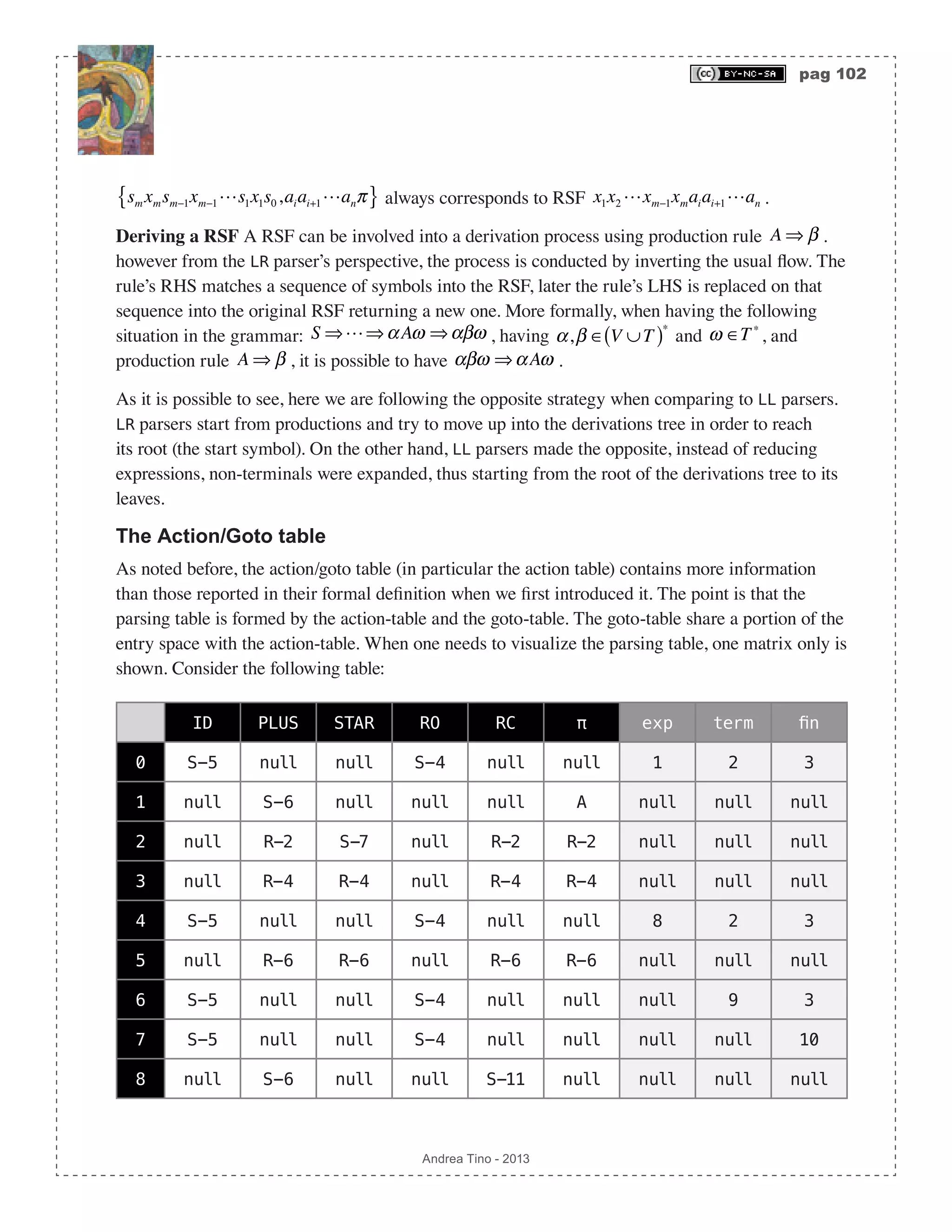
![pag 101 Andrea Tino - 2013 state is then pushed into the stack and will become the new top-state. All this will cause the parser to make a transition to state sm+1aism xmsm−1xm−1s1x1s0,ai+1anπ{ }. Please note how the look-ahead symbol is consumed. • Reduce: If the action is reduce, thus Action sm,ai( )= χR , then the action table will also return one more information: the production rule to use for reduction: A ⇒ β . So let r = β be the number of terminals and non-terminals in the rule’s RHS, then the stack will be shrunk by 2r elements by popping them. In particular the following must hold: β = xm−r+1xm−r+2 xm , thus symbols xm−r+1,xm−r+2 xm will be popped from the stack together with their corresponding states sm−r+1,sm−r+2 sm . Rule’s LHS A will be pushed into the stack together with the next state calculated as s = GoTo sm−r ,A( ) and becoming the new top-state. The parser will move to configuration sAsm−r xm−rsm−r−1xm−r−1s1x1s0,aiai+1anπ{ }. Please note how the loookahead symbol is not consumed. • Accept: If the action is accept, thus Action sm,ai( )= χA , then the parser terminates successfully. • Error: If the action is error, thus Action sm,ai( )= χE , then the parser terminates reporting the problem occurred. As it is possible to see, tables can return more information than those introduced so far in their formal definition. Later in this chapter we will detail them. The LR(1) parsing algorithm When considering an input sequence, a LR(1) parser follows these steps: 1. The input buffer is initialized with the input sequence. The stack is initialized by pushing the initial state. At the end of the initialization process, the parser’s state will be: s0,a1a2 anπ{ }. 2. Evaluate Action sm,ai( ) where sm is always the top-symbol in the stack. Accordingly to the action, the parser will act as described before. 3. Repeat point 2 until an error is found or until an accept action is performed. The algorithm needs certain types of grammars, ambiguities can be considered here as well. Right sentential forms A concept is very important in the context of LR parsing. [Def] Right sentential form: Given a grammar G V,T,P,S( ) and a sequence of symbols α ∈ V ∪T( )∗ , we call it a Right Sentential Form (RSF) for the grammar when the sequence can be written in the form: α = β1β2 βma1a2 an having βi ∈ V ∪T( ),∀i = 1…m and ai ∈T,∀i = 1…n , thus the right side is always filled with terminals. Recalling the concept of state for a LR parser introduced before, the state of a parser](https://image.slidesharecdn.com/creatingacompilerforyourownlanguage-150105162410-conversion-gate01/75/Creating-a-compiler-for-your-own-language-101-2048.jpg)
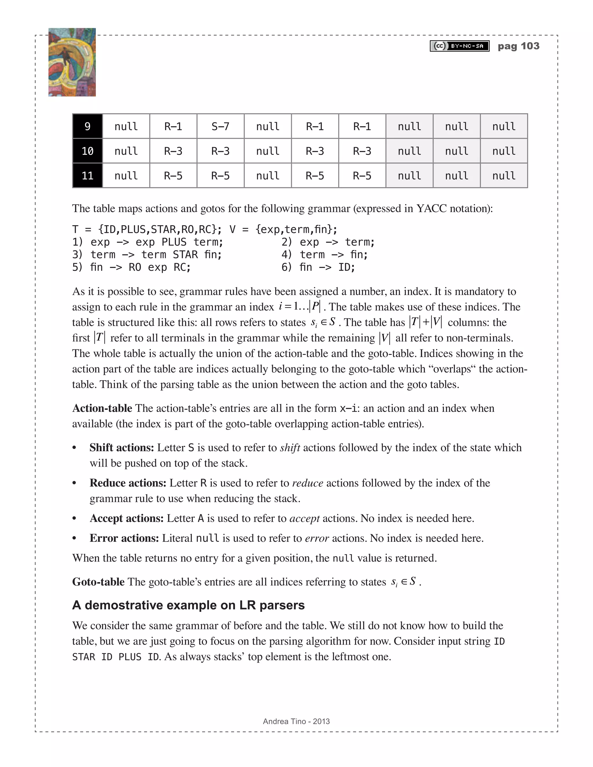
![pag 104 Andrea Tino - 2013 Stack Input buffer LA symbol Action [index] Descrirption {0} {ID,STAR,ID,PLUS ,ID,π} null reduce-0 Initialization. {5,ID,0} {STAR,ID,PLUS,ID,π} ID shift-5 Action-table returns shift. Symbol and state pushed. {3,fin,0} {ID,PLUS,ID,π} STAR reduce-6 Reducing using rule 6. Rule’s LHS is used to get next state. {2,term,0} {ID,PLUS,ID,π} STAR reduce-4 Reducing using rule 4. {7,STAR, 2,term,0} {ID,PLUS,ID,π} STAR shift-7 Shifting and pushing ele- ments in the stack. {5,ID,7,STAR, 2,term,0} {PLUS,ID,π} ID shift-5 Shifting and pushing ele- ments in the stack. {10,fin, 7,STAR, 2,term,0} {ID,π} PLUS reduce-6 Reducing using rule 6. {2,term,0} {ID,π} PLUS reduce-3 Reducing using rule 3. Stack gets shrunk! {1,exp,0} {ID,π} PLUS reduce-2 Reducing using rule 2. {6,PLUS, 1,exp,0} {ID,π} PLUS shift-6 Shifting. {5,ID,6,PLUS, 1,exp,0} {π} ID shift-5 Shifting. {3,fin,6, PLUS,1,exp,0} {} π reduce-6 Reducing using rule 6. {9,term,6, PLUS,1,exp,0} {} π reduce-4 Reducing using rule 4. {1,exp,0} {} π reduce-1 Reducing using rule 1. {} {} null accept Success! The whole process is very simple. The core part of the algorithm resides in the table. How to build parsing tables When we introduced LL grammars we also introduced parsing tables for them. A theorem can also be considered in order to decide whether a grammar is LL by inspecting the parsing table generated by that grammar. Here is the same. A grammar generates a parsing table which is](https://image.slidesharecdn.com/creatingacompilerforyourownlanguage-150105162410-conversion-gate01/75/Creating-a-compiler-for-your-own-language-104-2048.jpg)
![pag 105 Andrea Tino - 2013 supposed to have a certain structure. [Theo] LR grammars: A grammar is LR when the Action/Goto table can be built. There are some algorithms to build the parsing table for a LR grammar, it mostly depends on the specific case (in particular, the number of look-ahead symbols). The parsing algorithm is deeply related to the parsing table. Some important considerations The stack plays a key role; in fact it contains all information regarding the parsing itself. But what’s important to underline here is the fact that the whole stack is not necessary to parse a string; the top-state contains all information we need to make the parsing. So a LR parser just needs to investigate the top-state instead of the whole stack. This means that a FSA can be built out of this system. States are pushed into the stack and the stack is reduced only depeding on the top-state. A FSA will rule make the algorithm proceed until an accepting state is reached; the stack will help the FSA with all information it needs. So here it is: a pushdown automaton! We discovered nothing actually, as Chomsky and Schützenberger already told us that type-1 grammars are to be handled using such structures. Relating LR and LL grammars We understood that LL grammars are a subset of CFG grammars. What about LR grammars? [Lem] LR and CFG grammars: There exist non-LR CFG grammars. So, again, LR grammars are a subset of CFG grammars. But what can we say about LL and LR grammars when comparing them both? From what we could understand before, we found that LR grammars are parsed using pushdown automata. But LL grammars are parsed without the use of any FSA. Furthermore we know that type-2 grammars are handled using pushdown automata (recall the Chomsky-Schützenberger hierarcy). So it looks like LR grammars tend to be a little more generic than LL. [Theo] LR and LL grammars: LR grammars can describe LL grammars. LR(k) grammars can describe LL(k) grammars. So we have that LL grammars are a subset of LR grammars which are a subset of CFG grammars. This happens for one reason only: LL grammars are more restrictive than LR grammars. Recalling LL grammars, we need them to be non-left-recursive which is a strong requirement, LR(k) CFG LL(k)](https://image.slidesharecdn.com/creatingacompilerforyourownlanguage-150105162410-conversion-gate01/75/Creating-a-compiler-for-your-own-language-105-2048.jpg)
![pag 106 Andrea Tino - 2013 left-factorization is also required whenever predictive parsing is to be used. On the other hand, LR grammars, to be parsed, have ony one simple requirement: [Theo] Parsing LR grammars: LR(k) parsers can parse context-free grammars having one production rule only for the axiom. [Cor] Ambiguos LR grammars: Ambiguos grammars cannot be LR or LR(k). If the grammar has more than one production rule for the axiom S , we can create an equivalent LR grammar by simply adding a new non-terminal ′S ∈V , making it the new axiom and adding production rule ′S ⇒ Sπ . Also please note that the theorem provides a necessary condition only. LR(0) grammars and parsers The parsing algorithm is always the same, what changes is the parsing table, thus the action-table and the goto-table. How to build them? In this section we are going to see how to build these tables when handlind LR(0) grammars. LR(0) grammars are LR grammars using no lookahead symbols. These particular grammars are a little more restrictive than LR grammars, the parsing table can be built by analyzing the set of production rules. LR(0) items Item-sets A LR grammar must have some characteristics to be LR(0). By following certain methodologies it is possible to check whether a LR(0) can be generated out of a LR one. The first concept to understand is the LR(0) (dotted) item of a production rule. Given LR grammar G V,T,P,S( ) and a production rule, A ⇒ X1X2 …Xn , where Xi ∈V ∪T,∀i ∈1…n , the LR(0) item-set for that production rule is a set of production rules, all having A as LHS, in the form: A ⇒ X1Xi i Xi+1Xn ∀i = 1…n −1 iX1X2 …Xn X1X2 …Xn i ⎧ ⎨ ⎪ ⎩ ⎪ The dot • symbol is a new symbol added to the terminal set of the original grammar and becomes part of the new rules introduced by the item. When considering items for all production rules of](https://image.slidesharecdn.com/creatingacompilerforyourownlanguage-150105162410-conversion-gate01/75/Creating-a-compiler-for-your-own-language-106-2048.jpg)
![pag 110 Andrea Tino - 2013 3. For each final state, enter reduce in the action-column for that state in the table. Also specify the production rule by placing the rule index corresponding to the item in the state. If more items are present, put more indices (this is an ambiguity reduce/reduce). 4. The DFA must have a final state showing one item corresponding to rule ′S ⇒ iS . Replace the reduce action for that state with action accept. The table looks a little different when compared to LR tables, but both tables rely onto the same structures. Example Continuing the example of before, we can build the table following the algorithm. The table is: Todo Action ID PLUS STAR RO RC π exp term 0 shift S-5 null null S-4 null null 1 2 1 reduce null S-6 null null null A null null Please note how the action-table does not overlaps the goto-table. The parsing algorithm Compared to LR parsing described so far, LR(0) parsing is different because no lookahead symbols are needed. So the parsing algorithm described before needs to be modified just a little. Actually the procedure is always the same, but the action-table needs no character as input. It means that the action table does not overlaps with the goto-table. Also, to get the action, no character is needed, so the application becomes: Action :S Χ . The parsing algorithm remains the same. The next state is to be calculated using the goto-table as before, in this case the symbol in the stack is necessary. Conditions for LR(0) grammars Some important considerations can be made, in particular a very important result is reported below: [Theo] LR(0) grammars: A LR grammar is LR(0) if and only if each state in the CFSM is: a reduction state (final state) containing one reduction-item only, or a normal state (shift state) with one or more items in the closure (no reduction-items). [Cor] LR(0) grammars: A LR(0) grammar has one element only in each entry of the parsing table LR(1) CFG LR(0)](https://image.slidesharecdn.com/creatingacompilerforyourownlanguage-150105162410-conversion-gate01/75/Creating-a-compiler-for-your-own-language-110-2048.jpg)
![pag 111 Andrea Tino - 2013 This clearly makes LR(0) grammars a little more specific than LR grammars. So we can make our hierarcy a bit more precise by adding these grammars and placing them in the right position. SLR(1) grammars and parsers LR(0) grammars are very compact, but the lack of look-ahead symbols makes them inefficient sometimes. They can be improved with little efforts. SLR(1) parsers (Simple LR) work on a wider class of grammars as they allow the possibility to relax restrictions a little. Inserting look-ahead symbols SLR(1) parsers work with LR(0) parsing CFSM together with look-ahead symbols. Look-aheads are considered and generate modifications in the CFSM. In particular lookaheads are considered for items in states/closures in the DFA, but how to get look-aheads? For each item in states/closures of the DFA we have: • When having shift-items (non-reduce-items) in the form A ⇒α i β , look-aheads are all terminals in First β( ). • When having reduce-items in the form A ⇒α i , look-aheads are all terminals in Follow A( ). This will cause more transitions to be generated from the original CFSM. Solving ambiguities Sometimes SLR(0) grammars can help resolving LR(0) parser conflicts generated by ambiguities in the corrersponding LR(0) grammar. The approach is using look-ahead symbols to bypass ambiguities; however not always such an approach is successful. Not an exact methodology Using look-aheads in the follow-set of reduction-items is a good strategy, but definitely not always the best especially when handling shift/reduce conflicts. This is due to the fact for which using parsers embodying look-ahead symbols in their implementation is a far more precise approach than estimating them using follow-sets. Characterizing SLR(1) grammars We have the following important result: [Theo] SLR(1) grammars: A LR grammar is SLR(1) if and only if each state in the CFSM (augmented with look-aheads) is: a reduction state (final state) containing only one reduction-item per look-ahead symbol, or a normal state (shift state) with one or more](https://image.slidesharecdn.com/creatingacompilerforyourownlanguage-150105162410-conversion-gate01/75/Creating-a-compiler-for-your-own-language-111-2048.jpg)
![pag 112 Andrea Tino - 2013 items in the closure (no reduction-items). We know that ambiguos grammars cannot be LR, the same goes here: [Theo] Ambiguos SLR(1) grammars: Ambuguos grammars cannot be SLR(1). Also, the following result helps us placing SLR grammars: [Theo] SLR and LR grammars: There exist LR non-SLR grammars. This means that SLR(1) grammars are a superset of LR(0) grammars. The proof is simple as SLR(1) grammars enhance LR(0) grammars. Simplifying more complex grammars SLR grammars can be very efficient and be able to catch several constructs of languages. LR(1) grammars generate complex DFAs, however very often designers oversize the problem as many LR(1) grammars are actually SLR(1)! DFAs shrinks a lot when using SLR(1) parsing compared to LR(1). In fact, SLR(1) grammars being parsed using LR(1) algorithms generate a DFA with many more states than SLR(1) algorithms. LR(1) grammars and parsers LR(1) grammars are parsed by including look-ahead symbols into the process. Differently from SLR(1) parsers and grammars, here look-ahead symbols are part of the process from the beginning, they are not considered later as an appendix or similar. LR(1) items LR(1) items are a little bit different from LR(0) items. Basically a LR(1) items are like LR(0) items, but they contain information about look-ahead symbols. An item appears in the following form: A ⇒α i β,a[ ]. The dot-symbol assumes the same meaning, but a look-ahead symbol (terminal) appears as well. What does it mean? An item now is to be intended like: “The RHS left part has been recognized SLR(1) LR(0) LR(1)](https://image.slidesharecdn.com/creatingacompilerforyourownlanguage-150105162410-conversion-gate01/75/Creating-a-compiler-for-your-own-language-112-2048.jpg)
![pag 113 Andrea Tino - 2013 so far, the left part is expected once the look-ahead is be encountered!“. An item can be represented as: A ⇒ x1x2 xi i xi+1xn,a[ ], where xi ∈ V ∪T( )∗ ,∀i = 1…n and a ∈T ∪ π{ }. Basically an item like A ⇒α i β,a[ ] is not so different from a LR(0) item, but this item A ⇒αi,a[ ] is more different as it is a reduce-item only when the specified terminal appears in imput. The end-terminal π appears as look-ahead symbol for the axiom rule. LR(1) closure of an item The LR(1) closure for an item ′p ∈ ′P is to be calculated differently from LR(0) closures. 1. Initialize the closure to the empty set and add the item itself to it: Closure ′p( )= ′p{ }. 2. For every item A ⇒α i Bγ 1,a[ ] in the closure, add all items in the form B ⇒ iγ 2,b[ ] (predict- items) for all terminals appearing in the first-set of expression γ 1a: ∀b ∈First γ 1a( ). Mark the item. 3. Repeat step 2 until all items in the set are marked. The procedure is different because it keeps track of look-aheads. Building the CFSM All considerations made before for LR(0) grammars are still valid here. Algorithm The algorithm tu build the DFA is still the same with very little modifications. When calculating closures, the LR(1) closure is to be used. Furthermore, at the beginning of the algorithm, the first item to consider is ′S ⇒ iS,π[ ]: its closure is the initial state of the DFA. Final states Another important aspect is the following: in order to have a valid parsing, the DFA should have all final states as those states having at least one predict-item in the closure. But this is something we already knew. Now we have one more condition: predict-items should always have the last-terminal π as look-ahead symbol. Building the parsing table Compared to LR(0) grammars, the table now will be a little different as the action-table will overlap the goto-table. It means that the action depends both on the current state and on the look- ahead symbol as well. Here too, all considerations made for the LR(0) parsing table building algorithm are valid. 1. For each transition arc si → sj marked with symbol X ∈V ∪T , enter index j ∈ in table entry i, X( ). So: GoTo i, X( ) ⊇ j{ }. 2. For each shift state’s outgoing transition arc si → sj marked with symbol X ∈V ∪T , enter shift in action-table entry si , X( ), in the goto-table at the same entry place value j . 3. For each final state si , for each reduce-item A ⇒αi,a[ ], enter reduce in action-table entry](https://image.slidesharecdn.com/creatingacompilerforyourownlanguage-150105162410-conversion-gate01/75/Creating-a-compiler-for-your-own-language-113-2048.jpg)
![pag 114 Andrea Tino - 2013 si ,a( ). Also specify the production rule by placing the rule index corresponding to the item in the state, thus A ⇒α . If more items are present, put more indices (this is an ambiguity reduce/ reduce). 4. The DFA must have a final state showing item ′S ⇒ iS,π[ ], corresponding to rule ′S ⇒ iS . Replace the reduce action for that state with action accept. The procedure is very similar as it is possible to see. The parsing algorithm Parsing is performed as explained at the beginning of this chapter during the example. Characterizing LR(1) grammars We have the following important result: [Theo] LR(1) grammars: A LR grammar is LR(1) if and only if each state in the CFSM is: a reduction state (final state) containing only one reduction-item per look-ahead symbol, or a normal state (shift state) with one or more items in the closure (no reduction- items). We know that ambiguos grammars cannot be LR, the same goes here: [Theo] Ambiguos LR(1) grammars: Ambiguos grammars cannot be LR(1). LALR(1) grammars and parsers Let us focus on the last method to build parsing tables for LR grammars: LALR (Look-Ahead LR grammars). Here as well, these grammars can be more compact and generate smaller tables compared to canonical LR. The same goes for the CFSM which shrinks and needs less states. LR, SLR and LALR SLR grammars were introduced almost the same way as we are doing for LALR. However SLR grammars cannot catch many constructs that LALR can, yet both grammars have the same important characteristic: they generate smaller DFAs and more compact tables compared to canonical LR. However one result, which will be detailed later, is very imprtant: [Theo] LALR and SLR grammars’ CFSM sizes: LALR tables have the same number of states of SLR tables; although LALR grammars cover more constructs of SLR grammars.](https://image.slidesharecdn.com/creatingacompilerforyourownlanguage-150105162410-conversion-gate01/75/Creating-a-compiler-for-your-own-language-114-2048.jpg)
![pag 115 Andrea Tino - 2013 Please remember that table size is related to the number of states in the CFSM and vice-versa. Saying that the CFSM shrinks is the same as saying that the table gets more compact and smaller. The idea behind LALR parsing The idea behind is the same which drove SLR parsers: simplifying LR canonical parsers. The concept of core We need to introduce a quantity: the core of an item. Given a generic LR item A ⇒α i β,a[ ], we say that its core is the augmented grammar rule A ⇒α i β inside it, thus descarding any lookahead symbol (remember that when handling items, a new grammar is considered). Which means that LR(0) items’ core is the item itself. An interesting fact If we considered some generic LR grammar and the set of items built for the CFSM (closures), we would probably find closures where items have the same cores like items A ⇒ ia,a[ ], A ⇒ ia,b[ ] (as part of one state) and A ⇒ ia,π[ ] (into another different state) for example. When such states are encountered the action to perform is based on the lookahead symbol (the only one element making items different in this context). These two states could be merged into one state as they all imply a shift operation. Actually LALR(1) parsers work exactly this way: they reduce the number of states by merging LR(1) states generating smaller tables. Merging LR(1) states As anticipated before, the process basically consists in merging LR(1) states, but when can we perform this? The operation is possible only when states/closures contain items having the same set of cores. Attention, to be merged, two states si and sj must fulfill these conditions: 1. Evaluate the first state/closure and locate all cores. Put all cores into set Ri . 2. Evaluate the second state/closure and locate all cores. Put all cores into set Rj . 3. If both sets are equivalent: Ri = Rj , then the two states can be merged. The new state will contain all items contained in the orginal states. However now a problem arises: the CFSM has shrunk, the number of states has decreased but the table needs to be synched! What to do? What about the action of the new state? What about the goto of the new state? Setting actions and goto of merged LR(1) states There is a mapping between the parsing table (action-table + goto-table) and the CFSM. When a merge occurs, the tables must be re-shaped to keep synchronization. Synching the goto-table When two states are merged into the DFA, we need to handle transitions, which is equivalent to saying that the goto-table must synched! Actually the merging does not cause any problem in goto-table synching, the process is always successful.](https://image.slidesharecdn.com/creatingacompilerforyourownlanguage-150105162410-conversion-gate01/75/Creating-a-compiler-for-your-own-language-115-2048.jpg)
![pag 116 Andrea Tino - 2013 X1 X2 ... Xm s_i v_i_1 v_i_2 ... v_i_m ... ... ... ... ... s_j v_j_1 v_j_2 ... v_j_m X1 X2 ... Xm s_ij w_1 w_2 ... w_m ... ... ... ... ... Let us consider a generic entry for the same symbol in the original table for both states (to be merged): v_i_k and v_j_k which point to the next state. We can have two possibilities: • Both values are the same: v_i_k = v_j_k. In this case, no problem if both states for the same symbol lead to the same state it is ok, we have that w_k = v_i_k and that’s all. • Values are different. However this condition cannot occur. Let us consider absurdly to have two mergeable sets having transitions to two different states on the same symbol X , this condition is not possible because the items causing the transitions must share the same core (they cannot lead to two different states), thus such a condition is not possible. The goto-table can be managed always without problems. Synching the action-table The goto-table is never a problem. Problems can occur when trying to re-shape the action-table. In fact the action to set for a table entry depends on the value of each state, thus on items inside each closure. For example we might merge two states having different actions, what to do in that case? Conflict might occur. We will discover that shift/reduce conflicts will never occur (if the original LR(1) parser had no conflicts). However reduce/reduce conflicts might occur. No shift/reduce conflicts Let us consider a LR(1) parser having no conflicts, so a proper parser for a proper LR(1) grammar. If two states are merged into one state, it means they share the same set of cores. Let us consider two hypothetical states: s1 = core1,a[ ], core2,b[ ]{ } (a reduce state since we need to create a shift/reduce conflict) and s2 = core1,c[ ], core2,d[ ]{ } (a shift state). They must share the same cores as they are mergeable and inside each state, items generate no conflicts. The only possibility to have item core1,a[ ] to be in conflict with item core2,d[ ]. But if they generate a shift/reduce conflict it means that core1,a[ ] is in shift/reduce conflict with core2,b[ ] because item core2,b[ ] has the same core of item core2,d[ ], this would imply that the conflict originated in the first state first, but this is absurd as we considered the initial LR(1) as not ambiguos! This proves we cannot have shift/reduce conflicts. Reduce/reduce conflicts However, as anticipated, reduce/reduce conflicts can be experienced! Cores are the same but look-aheads are different! In that case we have conflicts and the grammar](https://image.slidesharecdn.com/creatingacompilerforyourownlanguage-150105162410-conversion-gate01/75/Creating-a-compiler-for-your-own-language-116-2048.jpg)
![pag 117 Andrea Tino - 2013 is not LALR(1)! Building the LALR(1) table We have already seen how to build the parsing table starting from the LR(1) table of the original LR(1) grammar: this is a valid approach but, although the simplest but the most time-expensive, definitely not the only one. A more efficient and advanced algorithm allows the construction of the LALR(1) CFSM without the LR(1) DFA. However, the advanced approach will not be covered here. To build the parsing table we start from the LR(1) parser, we shrink its CFSM and edit the original table. From a sistematic point of view, the following actions must be performed: 1. Consider all states in the LR(1) CFSM: s0,s1sn{ }, and locate all those having common sets of cores. 2. Merge states having the same set of cores obtaining a new set of states: r0,r1rm{ }. 3. For each new state, the corresponding value in the action-table is calculated with the same exact procedure used for LR(1) DFAs. 4. The goto table is filled as seen before, no conflicting values will be as all items in merged states have the same set of cores. This procedure is quite expensive and not efficient, but it is a valid approach. Characterizing LALR(1) grammars We have the following important result: [Theo] LALR(1) grammars: A LR grammar is LALR(1) if and only if each state in the reduced CFSM is: a reduction state (final state) containing only one reduction-item per look-ahead symbol, or a normal state (shift state) with one or more items in the closure (no reduction-items). [Cor] LALR(1) grammars: A LALR(1) grammar has one element only in each entry of the parsing table. We know that ambiguos grammars cannot be LR, the same goes here: [Theo] Ambiguos LALR(1) grammars: Ambiguos grammars cannot be LALR(1). LALR vs. LR LALR(1) grammars are more generic gramars than SLR(1), however not so powerful as canonical LR(1) LALR(1) SLR(1) LR(0)](https://image.slidesharecdn.com/creatingacompilerforyourownlanguage-150105162410-conversion-gate01/75/Creating-a-compiler-for-your-own-language-117-2048.jpg)
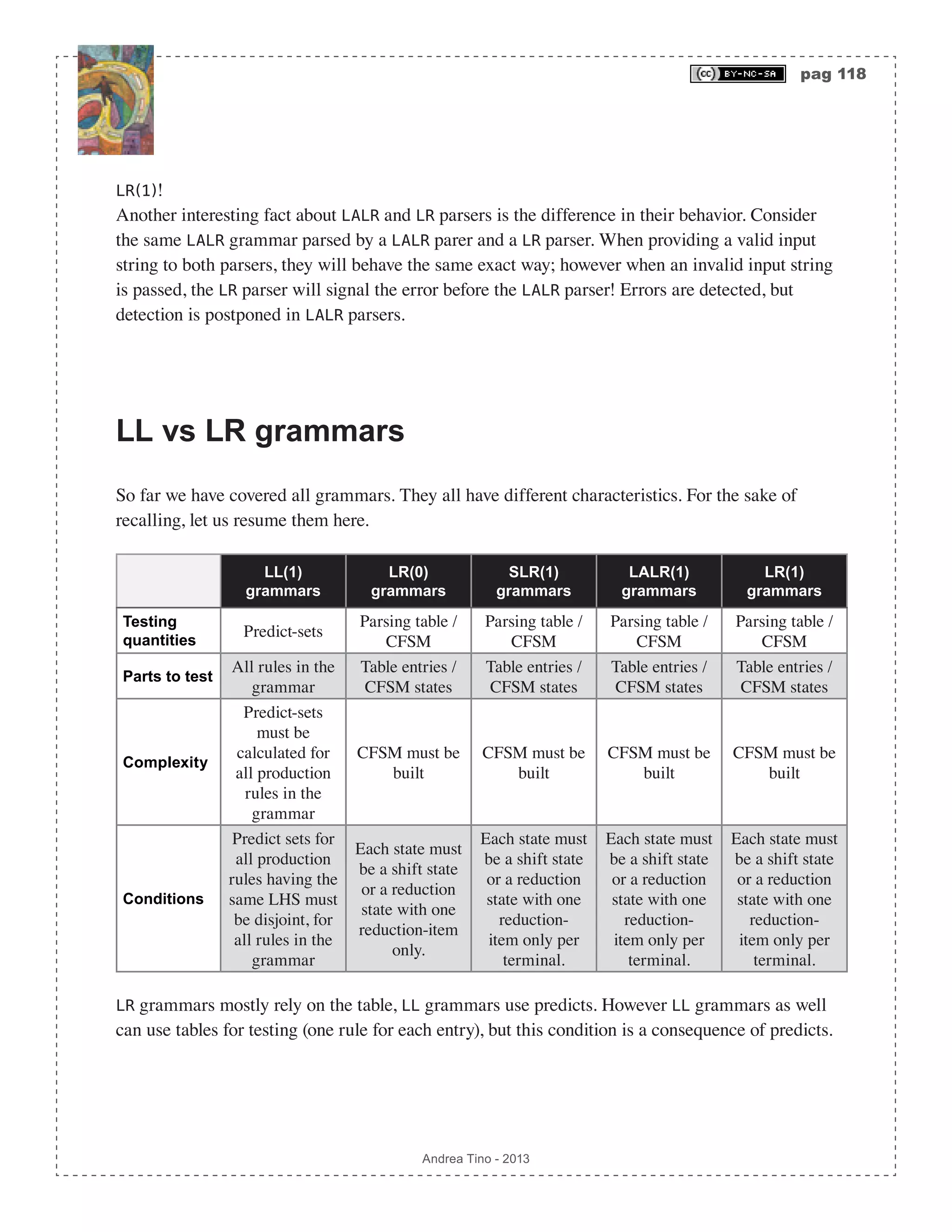
![pag 125 Andrea Tino - 2013 error occurs, the algorithm starts again from point 1. In pseudo-code we can write the algorithm as: procedure err_lrpanic(Stack,Table,Input) set StackCopy = Stack.clone(); do do if (not Table[Stack.top().state(),Input.current] = null) return; Stack.pop(); while not Stack.empty(); Stack = StackCopy; Input.next(); while not Input.empty(); report_error(“Could not recover!“); /* giving up :( */ end The algorithm is very similar to the one described before for LL parsers. LR phrase level method We introduced the phrase level approach during the introduction to this chapter. The methodology consists in modifying the input token which generated the error in order to make an attempt for a correct parsing. The idea When an error occurs the parser makes some attempts on the current look-ahead terminal in order to recover the parsing. The parser chooses some possible replacements to the current look-ahead. The basic idea is choosing replacements basing on the look-ahead which caused the error, since the error was due to the empty entry in the table for that specific terminal, replacements should make the parser point to a valid table entry (considering the current state at the top of the stack). 1. An error is detected because the table entry is null for the current state and the current look- ahead, the stack is saved into a temporary variable. 2. The parser considers the current look-ahead (which generated the error) and evaluates a set of terminals R = r1…rn{ }⊆ T that can possibly fix the input and that make the parser point to a valid entry in the goto-table given the current state. 3. Each replacement ri ∈R is used as new look-ahead (thus, discarding the original one). The parser tries to continue, if another error occurs, the replacement is discarded, the stack is recovered and the next replacement ri+1 ∈R is used until no more errors occur or the set of replacements becomes empty. In pseudo-code we can write the algorithm as: procedure err_phrasel(Stack,Table,Input)](https://image.slidesharecdn.com/creatingacompilerforyourownlanguage-150105162410-conversion-gate01/75/Creating-a-compiler-for-your-own-language-125-2048.jpg)
![pag 137 Andrea Tino - 2013 Dep p( )= Dep p,ω( ) ∀ω∈Attr X( ) ∀X∈p Graph of dependencies When an attribute is in the dependency-set of another attribute, a binary directed relation can be conidered between them. A graph can be built for dependencies in each production rule. A global graph for the grammar can be built when considering graphs generated for all production rules. Nodes in the graph are attributes. An arc connects two attributes in the graph ω2 → ω1 when there exists a semantic function calculating ω1 having ω2 as one of its arguments in the context of a production rule p ∈P , where symbols X1 ∈Σ ∪V and X2 ∈Σ ∪V , having ω1, X1( ) and ω2, X2( ) , are part of that production rule: X1, X2 ∈p. About the dependency graph The dependency graph collects all dependencies among all attributes for symbols in all production rules of the grammar. The graph is often represented on top of the AST; this approach is useful only when having an input string. However the dependencies can be visualized independently from derivations. To build the tree, the procedure is very simple: 1. List all semantic rules in the grammar for all production rules. 2. For each function ωi = fk µ1,µ2 …µi …µm( ), create a node for each attribute. Also create a arc ωi ← µj for all attributes as arguments of the function: ∀j = 1…m . Mark the rule. 3. Repeat point 2 until all rules are marked. Example of a dependency graph Todo Checking the presence of cycle-dependencies The dependency graph must be an acyclic graph for obvious reasons. If cycles were, then it would be impossible to calculate attributes part of that relationship. [Def] Acyclic attribute grammars: An attribute grammar is acyclic when its dependency graph is acyclic. The following result is obvious: [Lem] Parsing attribute grammars: An cyclic attribute grammar cannot be correctly parsed. Looking for cycles When investigating the dependency graph for a production rule it is easy to](https://image.slidesharecdn.com/creatingacompilerforyourownlanguage-150105162410-conversion-gate01/75/Creating-a-compiler-for-your-own-language-137-2048.jpg)
![pag 138 Andrea Tino - 2013 locate cycles, if any. However when merging all graphs for all rules, the final graph is much bigger and much more complex. The problem of cycles must be handled at the global level! It is not possible to check for cycles by investigating single rule’s graphs. [Theo] Acyclic rule graphs: If the dependency graph of a rule in an attribute grammar is acyclic, then the grammar is not said to be acyclic too. Please also consider the following results: [Theo] Acyclic graphs for more rules: Given a subset of rules in an attribute grammar, if their dependency graph (built as union of each rule’s graph) is acyclic, then the grammar is not said to be acyclic too. The whole graph must be considered to check the absence of cycles: [Theo] Acyclic grammars: Given the set of all rules in an attribute grammar, if their dependency graph (built as union of each rule’s graph) is acyclic, then the grammar is acyclic too. The vice-versa can be written as: [Theo] Acyclic subgraphs: If the dependecy graph of an attribute grammar is acyclic, then all dependency graphs of single rules in the grammar or dependency graphs of combinations of rules in the grammar are acyclic too. Equations We now know that the biggest graph must be inspected! Again we ask ourselves why an acyclic graph is needed, the answer was provided before: to be able to calculate all attributes. So, let us conside a generic dependency graph (it does not need to be the graph of the whole grammar, a single rule can do as well), and let us try to evaluate the values of all attributes. Let us introduce first the concept of semantic equation. [Def] Semantic equation: A semantic equation is a semantic function ωi = fk µ1…µm( ). The term equation is used to underline the fact for which calculations are needed to compute the value of attributes. [Theo] Existance of a solution for a system of semantic equations: If the dependency graph for a rule or a set of rules is acyclic, then the system of semantic equations derived from the graph has one solution.](https://image.slidesharecdn.com/creatingacompilerforyourownlanguage-150105162410-conversion-gate01/75/Creating-a-compiler-for-your-own-language-138-2048.jpg)
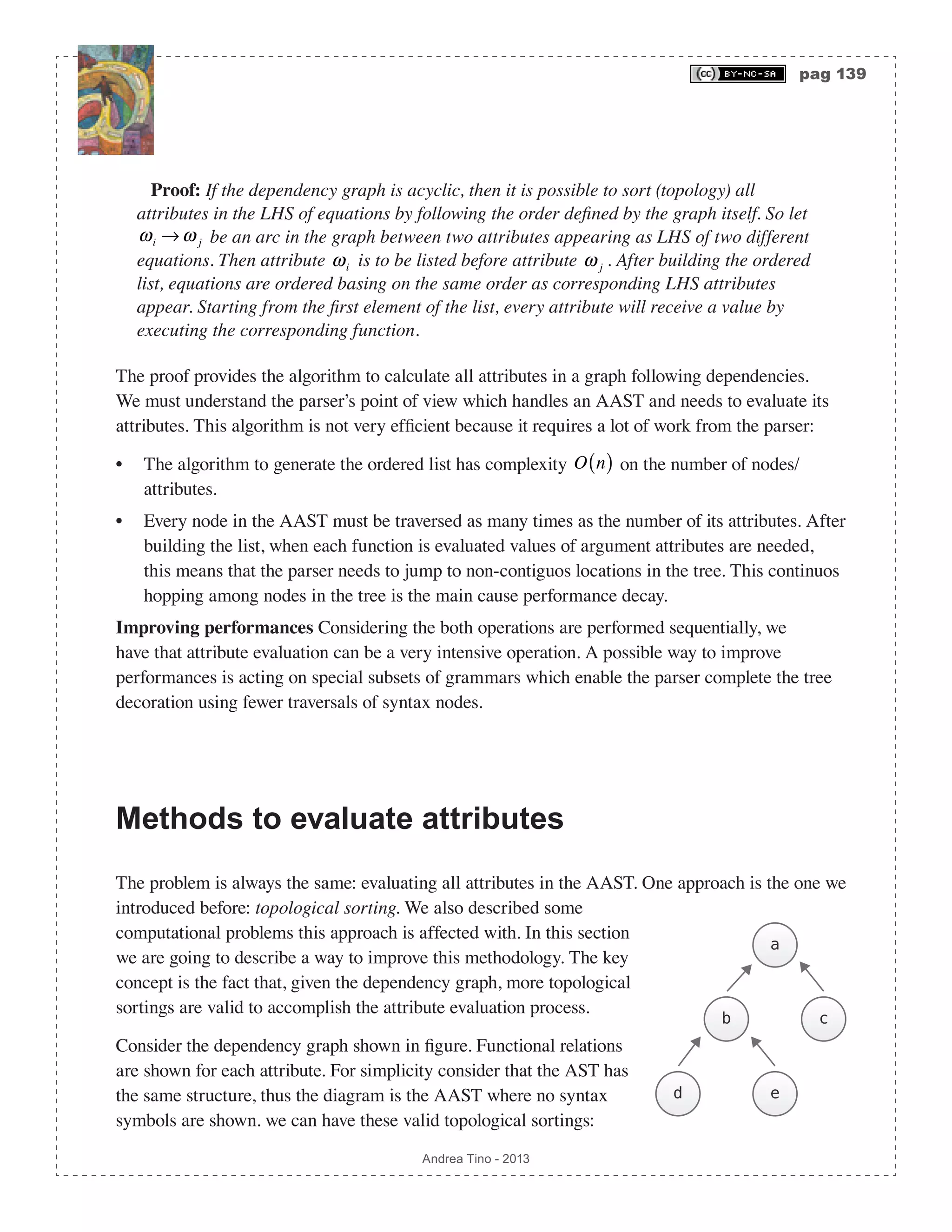
![pag 140 Andrea Tino - 2013 S1 = {d,e,c,b,a}; S2 = {e,d,c,b,a}; S3 = {c,e,d,b,a}; S4 = {e,c,d,b,a}; S5 = {d,e,b,c,a}; They are all valid because all functional dependencies are observed! There are more than one valid sorting because attributes are not completely ordered, thus there exist couples of attributes for which no particular order is defined. So which one to choose? Keeping in mind what we said before, sorting S5 is the best among listed! In fact when evaluating semantic actions following S5 sorting, the evaluator makes little traversals of the tree. The one described here is a possible improvement: its objective is minimizing the number of node traversals. Scheduling The evaluator is the component of a syntax-directed parser responsible for running the attribute evaluation process. We can have two different scheduling approaches: • Static scheduling: Scheduling is performed when the evaluator is built. Thus the scheduling depends on the grammar but not on the AST. A particular case is fixed scheduling: the sorting of attributes is the same for each production rule. • Dynamic scheduling: Scheduling is performed after the AST is built. Sorting of attributes is performed for every subtree generated by a production rule. Sweeps number Parsers can work using different approaches. Direct parsers build no AST and perform translation immediately. 2-step or classic parsers need to build the AST first and then traverse it. how many times is the tree to be traversed? 1-sweep parsers can traverse the tree one time only and translate the input code. However more complex grammars need more sweeps. The problems concenring sweeps number is purely related to semantics. The question is: “How many times does the semantic analyzer need to evaluate all attributes?“. In some cases more sweeps are needed to evaluate the value of all attributes in the tree. In syntax-directed semantics, two approaches are very common today: • S-attributed grammars: Only synthesized attributes are allowed. • L-attributed grammars: Synthesized and inherited attributes allowed, restriction on dependencies are considered. L-attributed grammars In order to make topological sorting more efficient, we can act on the grammar in order to be able to choose the best sorting. L-attributed grammars are a particular subset of attribute grammars with some properties. [Def] L-attributed grammar: An attribute grammar is L-attributed if all its production rules are L-attributed. [Def] L-attributed rule: A production rule A ⇒ X1X2 Xn of an attribute grammar is](https://image.slidesharecdn.com/creatingacompilerforyourownlanguage-150105162410-conversion-gate01/75/Creating-a-compiler-for-your-own-language-140-2048.jpg)
![pag 141 Andrea Tino - 2013 L-attributed if each attribute ωi, j of each RHS symbol Xi ∈Σ ∪V , having i = 1…n , only depends on attributes ωk,s ∈Ω of symbols Xk ∈Σ ∪V having k = 1… j −1 and from A ’s inherited attributes. Thus a L-attributed grammar is such that attributes for symbols depend on attributes of symbols on the left of each production rule’s RHS. This is a very strong restriction. Acyclic grammars Because of the structure of these grammars, we have a very important result here: [Lem] L-attributed acyclic grammars: L-attributed grammars are acyclic. Evaluating attributes How to calculate attributes in this grammar in a better way than topological sorting? A recursive descent left-to-right routine can work, actually this type of grammars can be correctly parsed using one sweep! This is the procedure: 1. Write a function for each production rule (whose LHS is a symbol in a node of the AAST). 2. Each routine takes two arguments: the subtree having as root the rule’s LHS symbol and all its inherited attributes. 3. When the value of an attribute is needed, a function calls that node’s function. The grammar is acyclic, thus recursive functions will never go loop. Using pseudo-code a possible implementation can be: Todo S-attributed top-down grammars Let us examine another class of grammars: top-down grammars where all attributes are synthesized attributes. How to handle attribute evaluation? The problem is that top-down parsing is such to create the AST from the root to leaves. Synthesized attribute describe an ascending flow. Directions of syntax and semantics are in contrast! We cannot parse the grammar without sweeping the tree at least one time! So this approach is not direct! Evaluating attributes using recursive-descent parsers Although conditions are such to make top-down and S-attributed grammars look incompatible, attributes can be evaluated without so many problems. Considering we want to treat generic LL(1) grammars, we are going to analyze how to handle recursive descent parsing: 1. For each function associated to a production rule (LHS), semantic functions for attributes of symbols in RHS are to be called after calling parsing functions for those symbols (non- terminals). 2. After gathering RHS attributes, attributes for LHS symbol can be evaluated.](https://image.slidesharecdn.com/creatingacompilerforyourownlanguage-150105162410-conversion-gate01/75/Creating-a-compiler-for-your-own-language-141-2048.jpg)
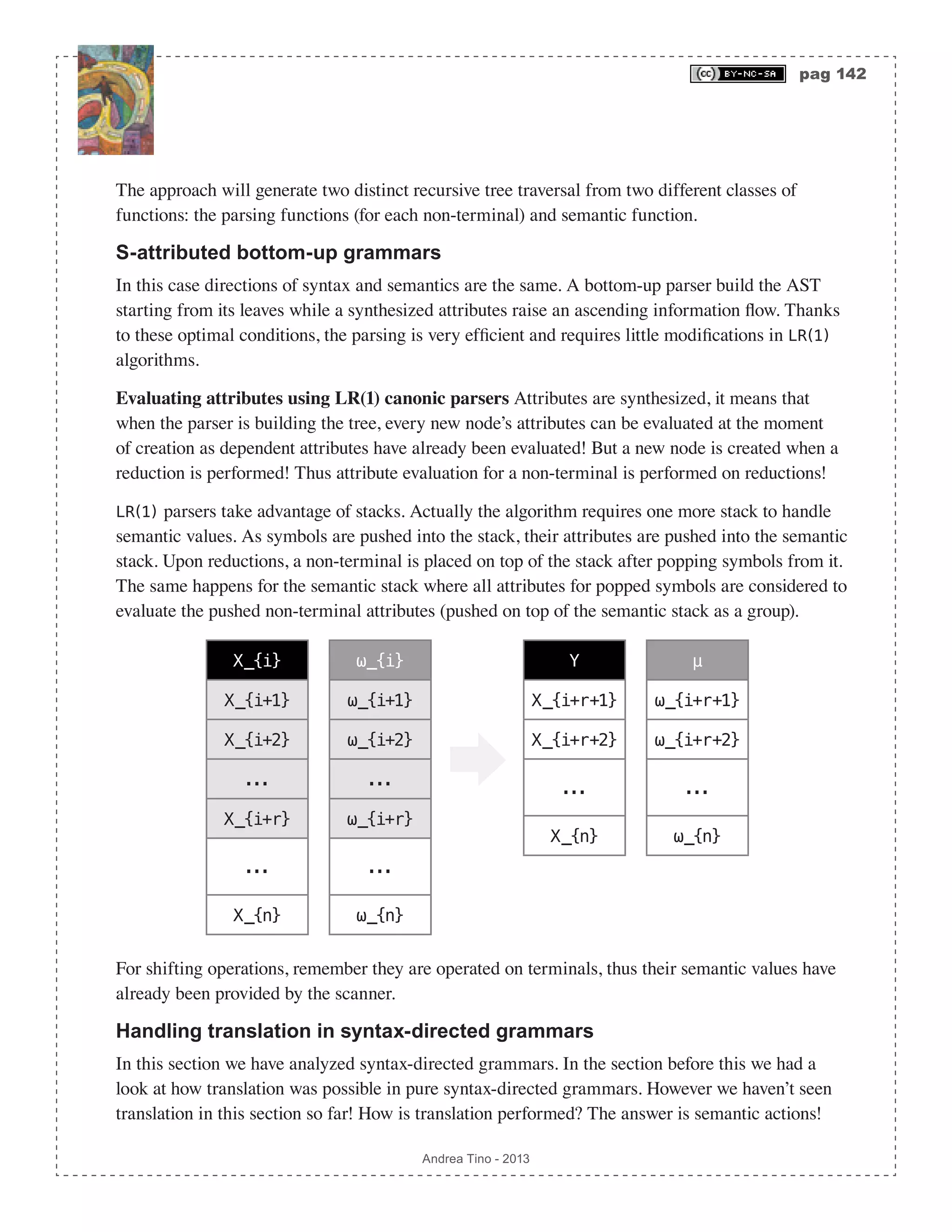
![pag 143 Andrea Tino - 2013 Semantic actions for translation We can do this using semantic actions. By placing output- write routine calls into semantic functions, we can write the output buffer as the parsing is being performed. Translation schemes Here we examine how to perform code translation. So far we have analyzed how to conduct parsing and semantic analysis together in one solution. Syntax-directed grammars gave us the possibility to make translation, however we had one limitation: we had no possibility to choose when a semantic action had to take place or, in case of more semantic actions for the same rule, in which order those actions had to take place. When needing a more fine-tuned syntax-directed translation, a subset of attribute grammars is considered: they are called translation schemes. [Def] Translation schemes: Translation schemes are attribute grammars where it is possible to explicitely define in which order semantic actions take place for every production rule. Important In the previous section we said that one attribute had to be handled by one semantic function only. It is right! We also defined semantic actions and semantif functions as the same thing. Here, this is valid no more. A semantic action is a routine which does not compute one attribute’s value, although it is associated to a symbol. On the other hand, semantic functions do evaluate one symbol’s attributes’ values. Please consider the following definitions. [Def] Semantic function: A semantic function is a semantic routine used to calculate the value of one attribute of one symbol. One attribute can have only one semantic function. one semantic function computes the value of one attribute only. [Def] Semantic action: A semantic action is a translation routine used to write the output buffer. One semantic action is associated to one symbol. One symbol can be associated with more semantic actions. In a translation scheme, this difference is important as it separates translation from semantics.](https://image.slidesharecdn.com/creatingacompilerforyourownlanguage-150105162410-conversion-gate01/75/Creating-a-compiler-for-your-own-language-143-2048.jpg)
![pag 146 Andrea Tino - 2013 • Dynamic semantics: Checking is performed at run-time. The compiler, while translating the input code to output, inserts calls to special routines meant to check parts of the code during execution. World is not black or white! Hybrid solutions exists as well, actually they represent the most common approach today. Type checking A language is said to be a typed language when every identifier is assigned an attribute called type. A type-value is just one possible value of the type attribute which can be associated to identifiers. [Def] Type system: In a compiler for a typed language, the type system is a collection of rules to assign a type to an expression involving identifiers and other entities to which a type is assigned. Type error When one rule in the type system is not observed, the compiler at compile time (static semantics) or the application at run time (dynamic semantics) can raise an exception. A type error is a condition for which one or more rules in the type system are not being observed. Type checker An important component of a type system is the type checker: a component whose objective is checking for type errors. Strongly typed languages A language is said to be strongly typed, when it gets compiled only if no type errors are found in it. Typed expressions The type system is used especially in those cases where an expression is to be assigned with a type. The expression is made of many identifiers and they all have a type. Which is the type of the expression? The type system can answer this question if no errors are found. Type expressions When assigning a type to an identifier or an expression, we do not always assign a simple type value, possible values for types can involve complex structures. Basic types for variables are simple types, for example int, float. A little bit more complex type expressions can be those involving new type, for example in C we can have enum myenum or struct mystruct. However in modern languages like C++ we can take advantage of templates, in that case we can refer to types by creating complex expressions like typename T::U. These are all type expressions. A possible list of type expressions can be: • Arrays, sequences or matrices. • Containers, composite data structures. • Pointers to other types.](https://image.slidesharecdn.com/creatingacompilerforyourownlanguage-150105162410-conversion-gate01/75/Creating-a-compiler-for-your-own-language-146-2048.jpg)
![pag 147 Andrea Tino - 2013 • Function pointers. • Generic programming, templates. The “type” attribute As we stated, in a typed language all symbols are assigned with a special attribute called type. This does not mean that all elements in the language have a type. Those symbols for which a type is not needed have their type attribute set to null. [Def] Type attribute: In a type system, every symbol is assigned with an attribute called “type“. The type attribute is a synthesized attribute and can own semantic actions and/or functions. Actions assigned to type attributes of symbols are typically used to check type attributes on which the original attribute relies on. So the type-checker can be implemented in tems of semantic actions. Checking type expressions Type checking is performed by analyzing type of more expressions and telling whether they are the same or not. Actually this is not the case for all possible conditions, but sure is a common case. So the question is: how can we recognize whether two types are the same? • Simple types: If the type values are simple types, the equivalence is immediate. For example: int = int, int != float, class A != class B, struct M = struct M. This happens because simple types are saved as basic types in the type system. • Type expressions: Type expressions are more complicated to handle. Actually the equivalence depends on the type system and its rules. More formally, the type system must include rules to check equivalence between type expressions. Type expressions equivalence We said that the type system must handle each case one by one according to its rules. Consider for example this fragment of C++ code: template <typename T> class TypeA { public: typedef typename T::U TypeAU; TypeAU member1; }; class TypeB { public: typedef unsigned int U; };](https://image.slidesharecdn.com/creatingacompilerforyourownlanguage-150105162410-conversion-gate01/75/Creating-a-compiler-for-your-own-language-147-2048.jpg)
![pag 149 Andrea Tino - 2013 expressions where operators, functions and user-defined types are involved, the type system must evaluate all user-defined operators and calculate the final type for the expression. In these cases, type errors usually disguise themselves as different error types. In C++ for example when an operator has not been overloaded for a user-defined type and a variable of that type is being manipulated using that operator, the compiler will not generate a type error, but a not-found function error. The “scope” attribute Another important attribute typically handled by semantics is the scope attribute. In many languages identifiers are assigned value, however the validity of this value is related to the scope of the variable. Understanding the concept of scope From a compiler’s point of view, scope is nothing more than a numerical value; from a language’s point of view, scope is a portion of the code where an identifier can be accessed by other parts of the code in the same scope. [Def] Scope: In a language (thus in a grammar), scope is the set of all couples of symbols having the same value for the “scope“ attribute. Be carefull: one thing is scope and another one is the scope attribute. The former is a concept, the latter is an attribute in a grammar. Scope checking Other than type checking routines, scope checking routines are considered by a compiler to check whether an identifier is being accessed by a partof the language in the same scope. Scope nesting Scopes are not disjoint sets. We can have nested structures. For the sake of scope checking, the scope attribute can be designed to be an array: two elements can be into different scopes, but one element can be in a scope contained by the other one; in that case that member is accessible.](https://image.slidesharecdn.com/creatingacompilerforyourownlanguage-150105162410-conversion-gate01/75/Creating-a-compiler-for-your-own-language-149-2048.jpg)
![pag 151 Andrea Tino - 2013 Overview Modern compilers treat all aspects of programming. When variables are declared and assigned a value, where is that value stored? Handling memory is a serious matter and can impact program execution performances. Memory allocation A compiler cannot decide on its own where to allocate a value. It must interface with the operating system and use system calls for some low-level operations. When a process is started, the operating system will reserve it a memory area where all its resources will be stored; the application code itself is stored into this area. Resource allocation can be performed in two flavors: • Static allocation: It is managed at compile time and depends by the code only. The total amount of memory required must be known at compile time. • Dynamic allocation: It s managed at run time, it depends both from the code and input parameters. It is not possible to evaluate the total amount of memory required by the program at compile time. To understand the difference between dynamic and static allocation we can consider array allocation. In static allocation it is not possible to create an array like this (dummy code): procedure MyProc(size) begin array MyArray[size]; end The size of the array is not known by the compiler until the program is executed and parameters passed by the user to it. The previous code, however, can be treated by a compiler supporting dynamic allocation. Static allocation The first language which introduced this strategy was Fortran77. Static allocation introduces a lot of limitations when programming, for example: • Arrays’ dimensions are to be known at compile time. • No recursive routines. • No composite structures without a fixed size. No expanding/shrinking containers. These languages can be very limitating but offer very high performances in exchange. Because of static allocation, all data is accessed in constant time. Furthermore there are no risks of memory overflow or out-of-memory errors at runtime.](https://image.slidesharecdn.com/creatingacompilerforyourownlanguage-150105162410-conversion-gate01/75/Creating-a-compiler-for-your-own-language-151-2048.jpg)
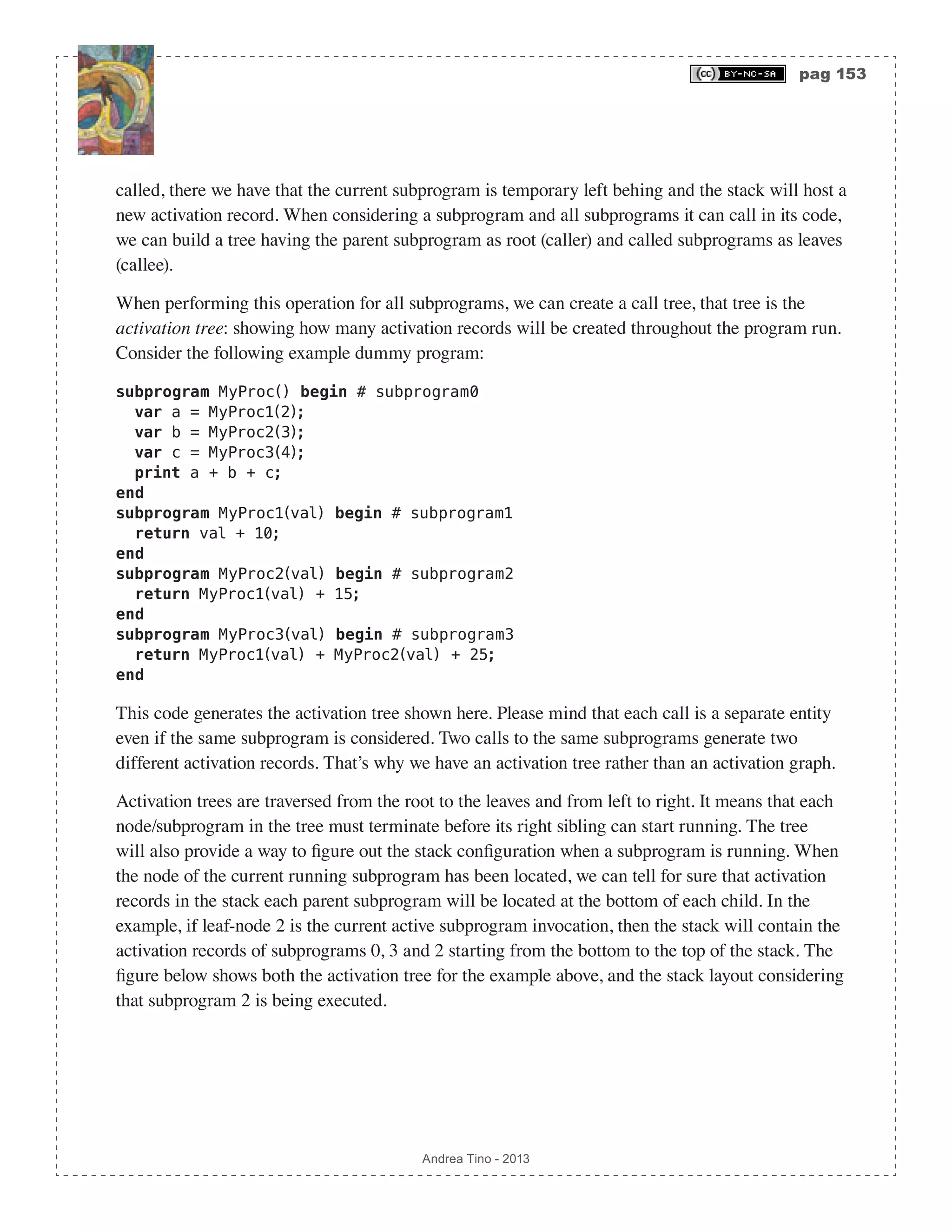
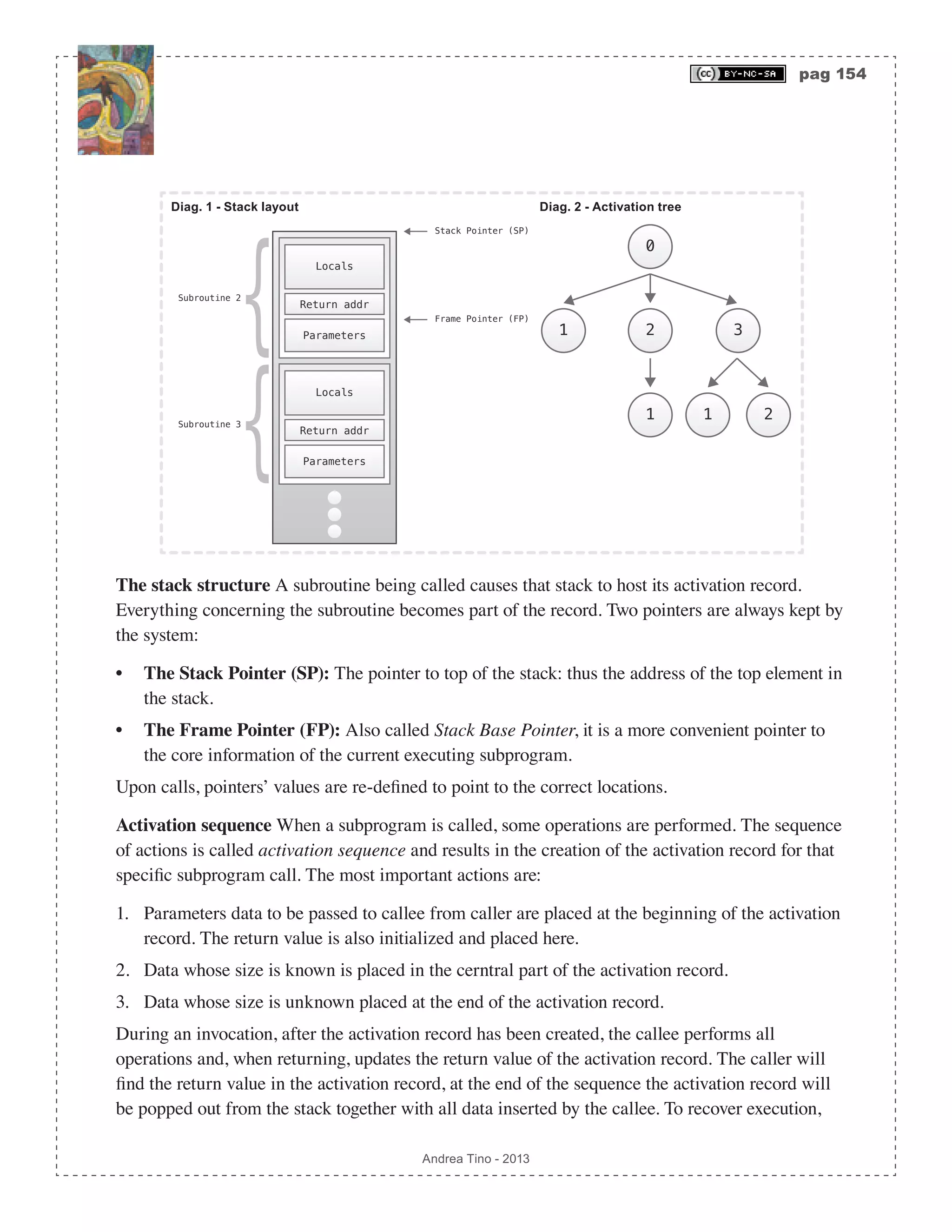
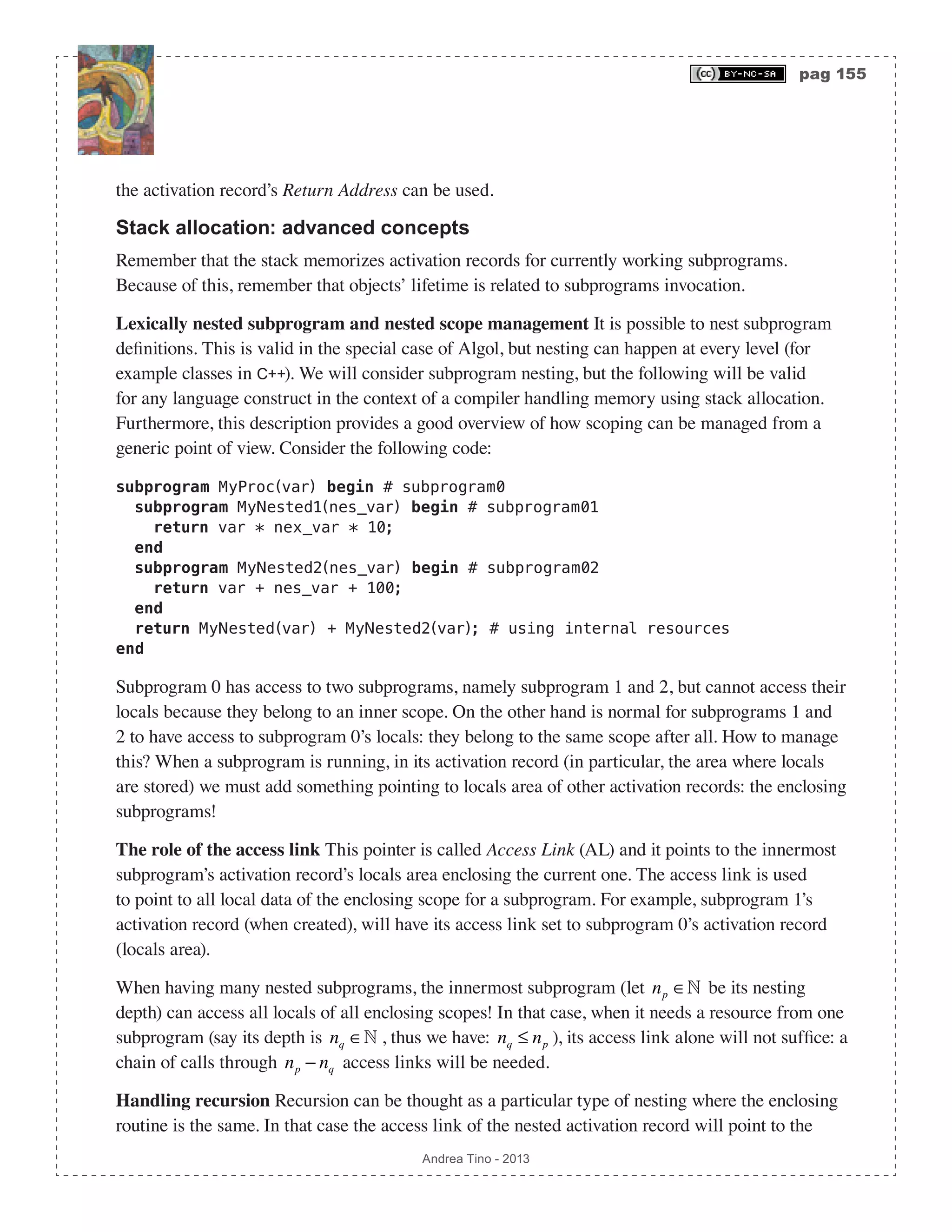
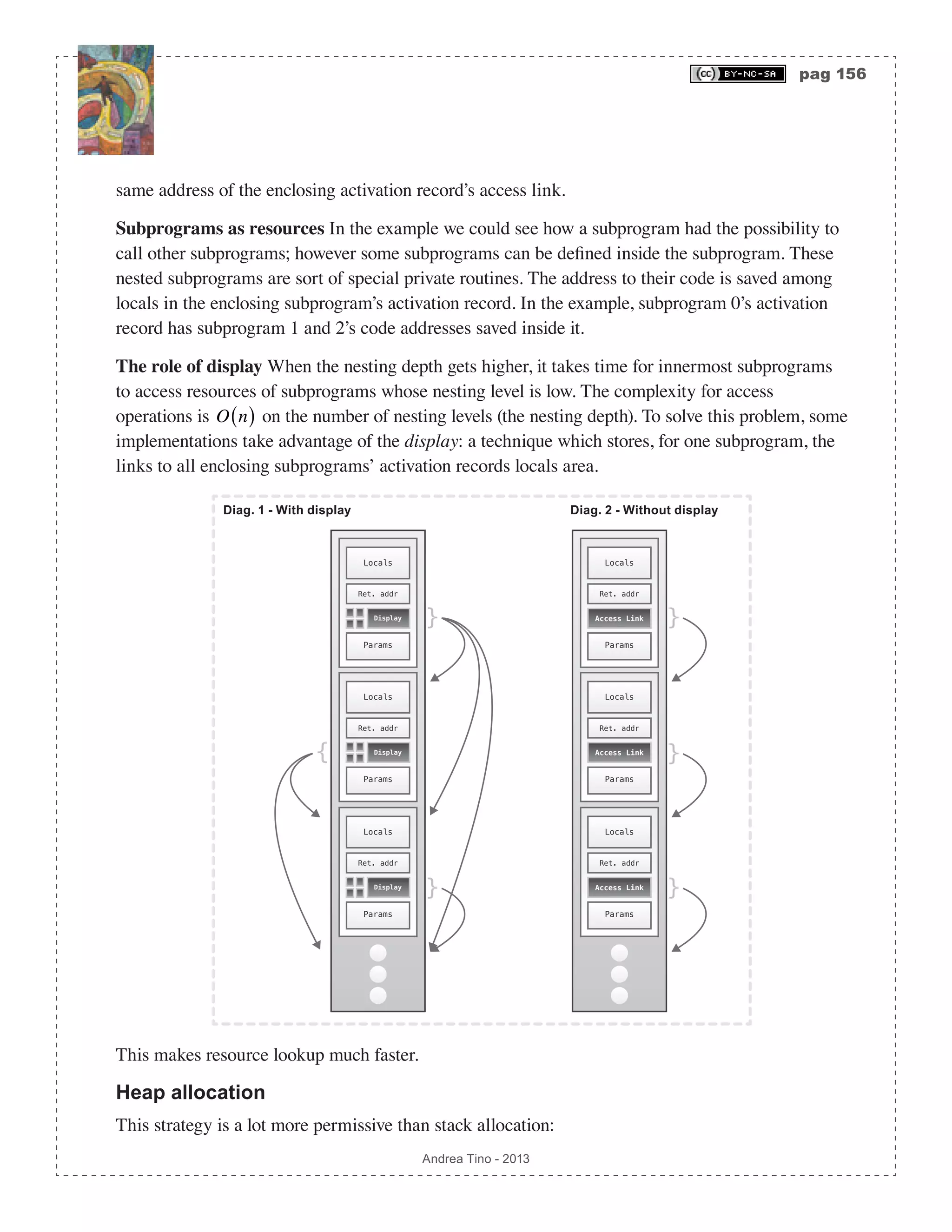
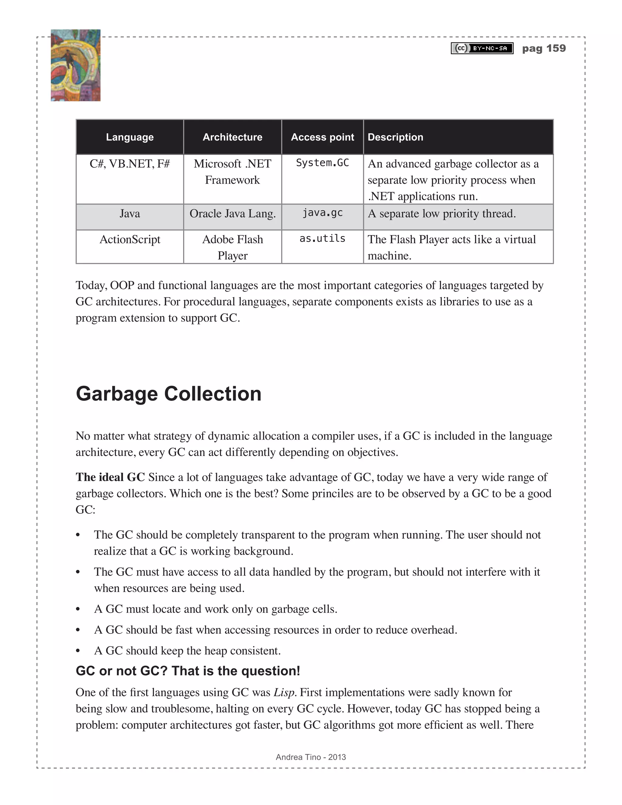
![pag 160 Andrea Tino - 2013 are still applications were a GC is incompatible (think of real time applications), but for normal programs the typical dilemma is: [Stat] The GC dilemma: Which is more important? Software which is free of memory leaks and allocation errors; or software which is a little faster but less reliable? Today’s GCs can provide solutions which can be a very good trade-off between the two counterparts of the afore-mentioned dilemma. We are now going to describe the most common GC strategies used today in many computer languages. GC through Reference Counting It was one of the most popular approaches to GC, it was adopted by Java (Sun Microsystems) and Microsoft COM (Component Object Model) as well. The idea The basic idea is equipping every heap cell (thus, objects) with a counter. This number will count the number of other objects pointing to that cell. If a graph of linked objects were to be drawn, the counter for each object would be equal to the number of incoming connections for that node. When the counter becomes zero, the cell must be collected. Problems The problem is that the GC complexity is distributed all over the heap on every single cell. When a cell is collected or a refernce updated/deleted, counters must be updated. So, given an object, how to located all objects linking the former? The problem is not simple. Implementation Thus every cell comes, together with a address, with a field called rc, the field stores a counter: the reference counter. To correctly handle counters for all objects in the heap, the following functions are considered: • Object creation: When a new object is created, its reference counter must be initialized to 1. • Object assignment: When an object is assigned to a variable, a new reference to that object is created. The counter must be incremented. • Object de-assignment: When a reference to an object is removed, the reference counter of that object must be decremented and zero-check be performed. • Object deletion: When an existing object is deleted, all reference counters of objects which were pointed by it must be decremented and zero-check performed for each one of them. • Zero-check: When issued, the checking routine checks whether the reference counter is 0 or not, in case it is 0, the cell address is inserted in the freelist. Everytime a new object is created or deleted or updated, the compiler emits calls to these functions in order to handle references.](https://image.slidesharecdn.com/creatingacompilerforyourownlanguage-150105162410-conversion-gate01/75/Creating-a-compiler-for-your-own-language-160-2048.jpg)
![pag 162 Andrea Tino - 2013 [Lem] Unreacheability in reference counting GC: In reference counting GC, unreacheable cells are cells whose reference counter becomes zero, or groups of cells, part of a reference cycle, whose reference counters all reached value 1. Trying to handle cycles Cycles can lead to memory leaks. How to deal with this? Reference counting alone cannot manage the situation, something more is necessary. Possible approaches can be: • The programmar must ensure that reference cycles are not created by the codes he writes. The compiler should detect cycles and return an error. • Combining reference counting with another garbage collection strategy. Advantages of Reference Counting Reference counting is not so bad after all. Some advantages can be considered. Easy to implement The strongest point sure its that reference counting is quite easy to implement. This makes the whole GC lightweight and fast as well. Homogeneous overhead As stated previously, overhead is distributed homogeneously on all computation. The GC does not start a collection cycle while blocking the program to check for garbage and collect it. The program itself updates references while running and garbage is automatically put in the freelist always by the program (thanks to some special routines emitted by the compiler when handling memory management instructions). The greatest part of the job is made by the running program, not by the GC! Space and time overhead As stated before, memory overhead is experienced because of the space required, for each cell, by the reference counter. Time overhead is experienced as well everytime reference counters must be updates. A particularly serious overhead is the one related to reference updates. When the pointer to an object is changed, a reference counter for an object must be decremented and the reference counter for the other one must be incremented. GC forgetfulness It is not that rare for the GC to forget updating reference counters. There are many reasons for this, but the consequences is the most important matter: • Forgetting to increment: When a reference counter is not incremented for an object, stange bugs can be experienced. Fragmentetion fault are to be experienced too, as the object might be collected when other objects still point to it! • Forgetting to decrement: This always leads to meory leaks as the object will persist in memory for the entire duration of the program run. If an object is removed and another object being pointed by it has not its reference counter updated, the latter will never be inserted in the freelist as a direc consequence.](https://image.slidesharecdn.com/creatingacompilerforyourownlanguage-150105162410-conversion-gate01/75/Creating-a-compiler-for-your-own-language-162-2048.jpg)


This document outlines the creation of a compiler for a programming language, detailing the design principles and theoretical foundations involved. It serves as a reference for students, emphasizing the importance of understanding compilers and interpreters, and covers topics such as compilation processes, optimization, and the classification of programming languages. The work is intended for engineering students and provides insights into the functionality of compilers and the necessary elements for their development.